行政院國家科學委員會專題研究計畫 期末報告
以長期風險模型結合貨幣政策探究利率的期限結構
計 畫 類 別 : 個別型 計 畫 編 號 : NSC 101-2410-H-004-028- 執 行 期 間 : 101 年 08 月 01 日至 102 年 07 月 31 日 執 行 單 位 : 國立政治大學金融系 計 畫 主 持 人 : 趙世偉 計畫參與人員: 博士班研究生-兼任助理人員:何昇晏 報 告 附 件 : 出席國際會議研究心得報告及發表論文 公 開 資 訊 : 本計畫涉及專利或其他智慧財產權,2 年後可公開查詢中 華 民 國 102 年 09 月 27 日
中 文 摘 要 : 本研究試圖將貨幣政策導入具有長期風險特質的資產訂價模 型,藉由債券市場均衡時貨幣政策利率與資產訂價利率必相 等的條件解出均衡狀態下之通貨膨脹與利率期限結構。以美 國資料進行的實證測定結果顯示:若中央銀行對於通貨膨脹 與實質經濟活動均積極回應,此模型可有效解釋正斜率的平 均殖利率曲線與負斜率的平均殖利率波動度曲線。若將此模 型的隨機折現因子以 Alvarez and Jermann (2005) 的方法 進行分解,亦可發現此模型對於債券風險溢酬的解釋能力明 顯優於採用外生性通貨膨脹的長期風險模型。然而,此模型 在解釋美國戰後不同貨幣政策時期的利率期限結構時,仍有 部分與實際資料不符的預測,有待進一步研究。
中文關鍵詞: 長期風險,貨幣政策,利率期限結構
英 文 摘 要 : Many previous studies of the term structure of interest rates specify the process for inflation exogenously. Because monetary policy is a crucial driver of inflation, this paper attempts to
endogenize the process for inflation through a
monetary policy rule and examines the performance of the model. Calibration results suggest that, given the strong stance of monetary policy, the model is able to explain the average upward-sloping nominal yield curve, volatile long rates and the downward-sloping term structure of volatility. The
decomposition of the nominal stochastic discount factor in the manner of Alvarez and Jermann (2005) also suggests that the negative correlation of equilibrium inflation and the monetary policy shock help to match the risk premium in the data. However, the model also has difficulty describing inflation and the term structure of yields across different historical regimes.
英文關鍵詞: long run risk, monetary policy, term structure of interest rates
1
Introduction
The dynamics of nominal interest rates is an important issue for economists and policy makers since it re‡ects future expectations for the economy. Empirical studies in past decades have established that the nominal yield curve is usually upward-sloping, the volatility of nominal yields has a downward-sloping term structure, and the term premia on long-term bonds are on average positive and time-varying. Some authors try to rationalize these stylized facts in equilibrium asset pricing models and gain some success, but most of them rely on an exogenous process for in‡ation in nominal bond pricing. This approach implies that in‡ation is not structural in these models, so the sources of in‡ation risk and the associated interest rate risk may not be clear. In addition, it is not possible to explore the role of speci…c in‡ation drivers, e.g., monetary policy, in the term structure of nominal yields if the in‡ation process is exogenous.
This paper attempts to address this issue by endogenizing the in‡ation process through a monetary policy rule in a consumption-based asset pricing model. If the conduct of monetary policy is a rule describing how the target of a short-term interest rate should be set in response to in‡ation and macroeconomic activity and the central bank commits to it, the market short-term yield should be adjusted so that it equals the policy target in equilibrium. According to this view, how the process for in‡ation is determined deeply a¤ects the term structure of interest rates. Economists have arrived at a consensus that in‡ation is ultimately a monetary phenomenon, and a large portion of the movements in in‡ation can be attributed to the conduct of monetary policy. Since a surge in in‡ation substantially depreciates the real payo¤s of long-term bonds, variations in monetary policy could be an important source of ‡uctuations in nominal yields. Hence the model proposed in this paper may help illuminate the role of monetary policy in shaping the term structure of interest rates.
The real side of the model features long-run risks and stochastic volatility in consumption dynamics. The recursive preference in the style of Epstein and Zin (1989) together with a high intertemporal elasticity of substitution implies that agents in this economy desire an early resolution of uncertainties. As indicated by Restoy and Weil (2011), this framework implies that asset risk premia are driven by covariances of asset returns with not only current
but also expected future consumption growth. As long as consumption growth and in‡ation are negatively correlated, a positive shock to long-run consumption growth volatility leads to the rise of the long-short nominal yield spread and bond risk premia. Thus the average yield curve is upward-sloping. In addition, this framework assumes a small but very persistent component and ‡uctuating uncertainty in real consumption growth. This component am-pli…es the consumption volatility channel so that the model can account for the magnitude and variation of bond risk premia quantitatively.
The nominal side of the model characterizes an endogenous in‡ation process that is jointly determined by the consumption dynamics and an interest rate feedback rule. The resulting model solution indicates that equilibrium in‡ation is triggered by the long-run consumption risk, stochastic volatility and monetary policy disturbance. Because the real payo¤ of any nominal asset is a¤ected by expected in‡ation, these components are also inherited to the nominal bond prices and yields. When long-run consumption growth and monetary policy shocks are quite persistent, the equilibrium nominal yields are highly autocorrelated and volatile. More importantly, the slowly diminishing impact of a monetary policy shock helps to explain the downward-sloping volatility curve of nominal yields and volatile long-term interest rates observed in the data.
Several recent studies have discussed the term structure of interest rates implied by the long-run risk framework. Bansal and Shaliastovich (2008) extend the model by Bansal and Yaron (2004) to resolve the predictability puzzles in bond and currency markets. Hasseltoft (2011) estimates a similar model through the simulated method of moments (SMM) ap-proach to seek joint explanations of key features of equity and bond markets. Doh (2011) incorporates a small persistent variation in the processes of both consumption growth and in‡ation to explore term structure of bond yields with Bayesian estimation. All of these works can account for some salient facts of yield curves, but their models rely on purely ex-ogenous processes of in‡ation. Thus the e¤ects of monetary policy on nominal yields are not clear in these models since the dynamics of in‡ation and real asset prices are independent.
Some authors have attempted to make the in‡ation process more structural in their recent works on consumption-based asset pricing models. Gallmeyer, Holli…eld, Palomino and Zin (2007) argue that a model with recursive preference and endogenous in‡ation can …t the
data more easily than one with exogenous information. However, they focus on comparing model performance and do not further explore the role of monetary policy in nominal yields. Gallmeyer, Holli…eld, Palomino and Zin (2009) develop another model with endogenous in‡ation to explain some salient facts of the term structure of interest rates. The workhorse of their model is a shock that is sensitive to consumption growth and non-systematic taste change, so their model does not feature any importance of long-run risks. Since risks for the long-run successfully explain some key facts of stock prices, it is worth examining if such a model with endogenous in‡ation is capable of describing the term structure of interest rates.1
Calibration with the postwar U.S. data reveals that a long-run risk model with endoge-nous in‡ation is able to explain several salient facts of nominal yields. First of all, the model captures the negative correlation of in‡ation and consumption growth in the data. The im-plication of this feature is that high expected in‡ation further depreciates the real payo¤s of nominal bonds when consumption growth is low. Thus nominal bonds are risky assets and carry positive risk premia. This explains why the average nominal term structure has a positive slope. Second, the volatility of consumption growth and monetary shock jointly generate volatile long rates and a downward-sloping term structure of volatility. In partic-ular, the monetary policy disturbance with an autoregressive process prevents the volatility of nominal yields from decaying too fast so that the model is able to match the volatility of long-term interest rates. Finally, the decomposition of the nominal stochastic discount factor in the manner of Alvarez and Jermann (2005) shows that the model risk premia are much closer to the consensus than those implied by the model with an exogenous process for in‡ation. This result comes from the negative correlation of equilibrium in‡ation and the monetary policy shock, which trims the risk premium on the long end of the term structure. Hence incorporating monetary policy helps to capture the risks implied by nominal yields more precisely.
On the other hand, sub-sample calibration results suggest that the model is not able to
1Models with long-run risks have more new developments recently. For example, Yang (2011) and Eraker,
Shaliastovich and Wang (2011) focus on long-run risk in durable consumption growth to explain key asset market facts. Dittmar and Palomino (2010) introduce leisure and wage in a long-run risk model and …nd more plausible results in explaining equity returns. To illuminate the role of monetary policy and keep the tractability of the model, I do not address these issues in this paper.
reconcile the historical regimes of monetary policy and the corresponding term structure of interest rates in some aspects. First of all, most studies of U.S. monetary policy suggest that the conduct of monetary policy was more e¤ective in controlling in‡ation after the 1980s, but the model implies the opposite because it requires somewhat passive monetary policy to reproduce more volatile nominal yields and a larger term spread in the Volcker-Greenspan era. This result may be attributed to the e¤ect of monetary policy on the process of in‡ation. The model implies that a more aggressive policy response to in‡ation reduces the volatility of in‡ation and nominal yields. Thus monetary policy moves the volatility of the two variables in the same direction. However, the data show volatile in‡ation and stable nominal yields in the 1970s and the opposite pattern since the 1980s. Hence it is not a surprise that the model fails to track the data.
Second, the term spread of nominal yields is on average larger since the 1980s while the model predicts that a stronger in‡ation stabilization policy reduces the term spread. In the model economy, in‡ation is endogenously determined through a credible monetary policy rule. A more aggressive policy response to in‡ation is interpreted as a clear sign of declining long-run risk, and in‡ation becomes less volatile. As a result, long-term bonds bear lower in‡ation risk premia and the term spread should get smaller. However, the data show that the term spread is on average increasing from Burns-Miller to Volcker-Greenspan. This conundrum might be attributed to a less credible monetary policy in the Greenspan era or other factors that are not related to monetary policy, as suggested by Polamino (2012). The model cannot account for these features since it assumes a commitment to the policy rule, and the factors unrelated to monetary policy are not well known.
Finally, the model requires a more than proportional rise in the short rate associated with the increase in consumption growth and in‡ation, namely, aggressive monetary policy, to replicate the level and slope of the nominal interest rates. Although this policy practice conforms to the Taylor principle and ensures the existence of a unique stationary equilibrium, the view that there has been a sustained strong policy response to in‡ation in the past decades gets very limited empirical support. Many studies of U.S. monetary policy, such as Clarida, Galí and Gertler (2000), Cogley and Sargent (2001, 2005) and Lubik and Schorfheide (2004), suggest that the Fed was passive in response to in‡ation in the 1970s. If the conduct
of monetary policy did not conform to the Taylor principle in the 1970s, it is not possible for the model to account for the upward-sloping yield curve in that period.
A more fundamental problem of the model regards the inconsistency between Euler equa-tion interest rates and money market rates. The model requires the equivalence of the two rates to clear the bond market and determine the equilibrium process of in‡ation. How-ever, an analysis by Canzoneri, Cumby and Diba (2007) indicates that many asset pricing models generate systematic negative correlation between the Euler equation rate and the Federal Funds rate. On the other hand, most contemporary central banks conduct mone-tary tightening by raising the target of a short rate. Thus the interest rates implied by the Euler equation of a model should also rise in response to this policy. However, the model implies that a positive monetary policy shock decreases the Euler equation rates and raises the money market rates based on the Fed’s policy reaction rule. This result stems mainly from the negative response of in‡ation to a monetary policy shock. Forcing this response to be positive cannot solve the problem since it counterfactually implies that disin‡ation policy exacerbates in‡ation. This inconsistency problem imposes a fundamental challenge to the long-run risk model with endogenous in‡ation.
2
Model
2.1
Consumption Dynamics
Consider an endowment economy in which agents have Epstein-Zin preferences: Ut= h (1 )C 1 t + EtU 1 t+1 1i1 ; (1)
where is the subjective discount factor, 0 is the risk aversion parameter, = (1 )=(1 1= ) and 0 is the intertemporal elasticity of substitution. Epstein and Zin (1989) derived that the associated logarithm of real stochastic discount factor (SDF) is:
mt+1= ln ct+1+ ( 1)rc;t+1; (2)
where ct+1 denotes the log of real aggregate consumption growth and rc;t+1 represents the
Yaron (2004):
ct+1 = + xt+ t t+1; (3)
xt+1= xt+ 'e t t+1; (4) 2
t+1 = (1 1) 2 + 1 2t + wwt+1: (5)
The log of real aggregate consumption growth is determined by an unconditional mean , a small persistent component xt and a short-run consumption risk t+1. The term xt follows
an autoregressive process with persistence parameter and a long-run consumption risk t+1.
To capture the time-varying bond risk premium, the model features a conditional stochastic volatility of consumption growth 2
t, which also follows an autoregressive process and is
subject to a macroeconomic volatility risk wt+1. The innovations to consumption growth
and stochastic volatility are assumed to have independent standard normal distributions.
2.2
Monetary Policy Rule
Unlike many previous studies, the equilibrium process for in‡ation in the model is closely related to the conduct of monetary policy. In this economy, the central bank considers movements of consumption growth and in‡ation to set the target of short-term interest rate it as follows:
it = i0+ ic ct+ i t+ ut; (6)
where t denotes the measure of in‡ation and ut characterizes the policy disturbance. The
coe¢ cients icand i measure policy responses to consumption growth and in‡ation,
respec-tively. The monetary policy shock is assumed to follow an autoregressive process:
ut+1 = uut+ t+1; (7)
where t+1 N (0; 1). Such a contemporaneous rule is close to the usual Taylor rule
speci…-cation. The major deviation is that the central bank responds to consumption growth rather than output gap as there is no production in this economy. The model with a contempora-neous monetary policy rule is denoted as Model C.
Some authors argue that the central bank should formulate interest rate decisions based on expected macroeconomic variables. For example, Clarida, Galí and Gertler (2000) propose
a forward-looking rule as follows:
it= i0+ icEt( ct+1) + i Et( t+1) + ut: (8)
The disturbance follows the same autoregressive process as (7). The model with a forward-looking monetary policy rule is denoted as Model F. Given that two speci…cations character-ize di¤erent reactions to macroeconomic conditions by the central bank, it is interesting to see whether they imply di¤erent equilibrium processes for in‡ation and interest rate dynamics.
2.3
Equilibrium In‡ation and Bond Yields
Given that the real SDF contains the unobservable return on aggregate wealth rc;t+1, the
…rst step of the solution procedure is to approximate this element using the method proposed by Campbell and Shiller (1988):
rc;t+1 = 0 + 1zt+1 zt+ ct+1; (9)
where zt denotes the log of price to consumption ratio, 0 and 1 are functions of z, and z
is the average of zt. Bansal and Yaron (2004) conjecture that zt is a linear function of two
state variables xt and 2t, i.e.,
zt= A0+ A1xt+ A2 2t; (10)
where the coe¢ cients A0, A1and A2can be solved using the Euler equation with consumption
dynamics.
The second step is to solve for the equilibrium process for in‡ation. Because in‡ation is determined through monetary policy, the short-term nominal interest rate derived from the nominal SDF should equal the policy target set by the central bank. Therefore,
it = Et(mt+1 t+1)
1
2V art(mt+1 t+1) ; (11) where the right-hand side is obtained by exploiting the properties of the log-normal distri-bution and t+1 depends on the speci…cation of monetary policy. The speci…cation of the
forward-looking policy rule and equation (11) lead to the following conjecture of t:
Thus the equilibrium in‡ation is linear in the state variables xt, 2t and ut. Similarly, the
conjecture of the equilibrium in‡ation in the case of contemporaneous policy rule is given as follows:
t+1 = 0+ xxt+ 2t + uut+ t t+1+ t t+1+ wwt+1+ t+1: (13)
The equilibrium process for in‡ation can be solved by plugging the real SDF and the con-jectured process for in‡ation into (11).
The …nal step is to solve for nominal bond prices and yields. Let pen
t denote the log price
of a zero-coupon nominal bond with maturity n at time t. In a frictionless economy, no arbitrage condition implies that the following Euler equation must hold:
Et exp mt+1 t+1+pen 1t+1 pe n
t = 1: (14)
Given that all disturbances are Gaussian, the Euler equation (14) can be written as Et mt+1 t+1+pen 1t+1 pe n t + 1 2V art mt+1 t+1+pe n 1 t+1 pe n t = 0: (15)
Based on the speci…cation of mt+1 and t+1, I conjecture that pent is linear in the three state
variables xt, 2t and ut, i.e.,
e
pnt = eB0n+ eBxnxt+ eBn 2t + eB n
uut; (16)
and the corresponding nominal yields eytn can be de…ned as e
ynt = 1 nep
n
t: (17)
The equilibrium bond prices can be solved recursively by plugging all dynamics into (15).
3
Model Calibration and Implications
To study the implications of the model, I calibrate the parameters in consumption dynamics and the monetary policy rule to match the moments of consumption growth, in‡ation and nominal yields. The data are U.S. quarterly series from 1952:2 to 2011:2. Consumption data are constructed using per capita consumption growth of nondurables and services from
the Bureau of Economic Analysis (BEA). In‡ation is measured using the price index that corresponds to consumption data, which is also available from BEA. Piazzesi and Schnei-der (2007) argue that this measure has less high-frequency noise than the commonly used consumer price index (CPI). Bond yields data are from CRSP Fama-Bliss discount bond …les.
The parameters are calibrated to match major moments of consumption growth and nominal term structure. Since monetary policy does not a¤ect consumption dynamics in the model, both Model F and Model C share the same real side parameters. Table 1 lists the calibrated parameter values. The value of corresponds to 1:97% per annum consumption growth for the entire sample period. Other parameters of consumption growth are chosen to match its volatility and …rst-order autocorrelation. Following Bansal and Yaron (2004), the intertemporal elasticity of substitution is set at 1:5. The choice of risk aversion parameter = 7:5 is comparable to those in the literature. Parameters of the monetary policy rule are chosen to match the average level and volatility of nominal yields.
3.1
Equilibrium In‡ation
Table 2 summarizes the moments of consumption growth and in‡ation. Model calibration shows that two speci…cations of the monetary policy rule yield similar in‡ation dynamics. The average quarterly in‡ation is 0:76% in Model F and 0:77% in Model C, and the asso-ciated volatility is 0:95% in Model F and 0:96% in Model C. Although in‡ation is slightly lower on average and somewhat more volatile compared to the data, these moments do not seriously deviate from the data since the calibration matches the moments of nominal yields given consumption dynamics. The model also overestimates the …rst-order autocorre-lation of in‡ation when the monetary policy is described by a forward-looking rule. Because equilibrium in‡ation is a function of consumption dynamics and monetary policy, its auto-correlation inherits the persistence from the state variables xt, 2t and ut. Highly persistent
consumption dynamics and monetary shocks result in a quite persistent process for in‡a-tion. This is more obvious in Model F since the central bank responds to future expected macroeconomic variables.
load-ings characterize how in‡ation is associated with the macroeconomic dynamics and various risks. First of all, equilibrium in‡ation is inversely related to the small persistent component in consumption growth, i.e.„ x < 0. Holding other things constant, this feature implies a
negative contemporaneous correlation of in‡ation and consumption growth. Given a pos-itive and large ic, the Fed substantially raises the short rate when consumption growth is
high. The aggressive policy reduces current and future in‡ation, so the model suggests a negative correlation between the two. Table 2 shows that corr( c; ) = 0:1762 in Model F and 0:2593 in Model C. In fact, the macroeconomic data reveal that this correlation is 0:1073. Thus the negative correlation of in‡ation and consumption growth is exactly what we observe in the data.
The coe¢ cients and u are also negative, which indicates that an increase in
uncer-tainty or an unexpected policy tightening decreases the equilibrium in‡ation. The intuition for < 0 is the behavior of precautionary saving. When future consumption growth be-comes more uncertain, agents in the economy tend to save more. This precautionary motive raises the demand for bonds and lowers the interest rates and in‡ation. The result u < 0
can be thought of as a consequence of the disin‡ation policy. Given the strong stance of the Fed on price stability, i.e., i > 1, an unexpected positive policy shock e¤ectively raises the interest rate and reduces in‡ation in current and future periods. Meanwhile, a negative u
also implies that an aggressive monetary policy dampens the volatility of in‡ation.
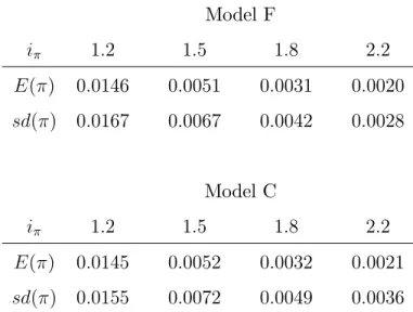
As equilibrium in‡ation is determined through a monetary policy rule, the conduct of monetary policy can a¤ect the dynamics of in‡ation. Table 3 reports how the mean and the standard deviation of in‡ation change with di¤erent values of i while all other parameters are kept at their baseline values. This ceteris paribus analysis shows that a larger value of i results in lower and more stable in‡ation. When i = 1:2, the average quarterly in‡ation is approximately 1:45% (or 5:8% per annum) and the standard deviation is 1:67%. If i = 2:2, the average quarterly in‡ation substantially shrinks to 0:2% (or 0:8% per annum) and the standard deviation also decreases to roughly 0:3%. Holding other things constant, the model suggests that a stronger policy stance on price stability does achieve a more desirable outcome.
3.2
The Term Structure of Nominal Yields
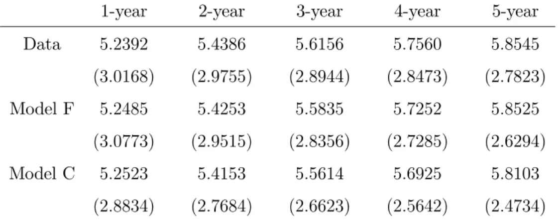
Table 4 reports the average nominal yield curve and the associated volatility. Given the consumption dynamics, the model reasonably matches the average level and variation for one- to …ve-year nominal yields. In addition, the model reproduces two important facts of the nominal interest rates. First, the average nominal term structure has a positive slope. The average one-year yield is 5:25% in Model F and Model C, then gradually increases to 5:85% in Model F and 5:81% in Model C for the …ve-year yield. Second, the average volatility of nominal yields has a downward-sloping term structure. The standard deviation of the one-year rate is 3:08% in Model F and 2:88% in Model C, then slowly decreases to 2:63% in Model F and 2:47% in Model C for the …ve-year rate. Thus the model captures the high variance of long-term yields in the data even if the volatility curve decreases in maturity. As documented in Shiller (1979), the volatile long-term interest rates imply the failure of the conventional expectation hypothesis.
To understand the upward-sloping average term structure of nominal rates, …rst recall that the equilibrium in‡ation is negatively correlated with current consumption growth. Since high in‡ation reduces the real value of any monetary payment, real payo¤s on nominal bonds are extremely poor in bad states. In addition, recursive preference implies that nom-inal bonds are also unattractive in times with news of unexpectedly high in‡ation. More explicitly, in‡ation is also bad news for future consumption growth. Thus risk-averse in-vestors demand positive risk premia on nominal bonds for compensation. As indicated by Piazzesi and Schneider (2007), this feature results in an upward-sloping nominal yield curve. It is worth noting that the above result requires an aggressive policy response to con-sumption growth. Because the relative risk aversion coe¢ cient is greater than the reciprocal of intertemporal elasticity of substitution in the model, the covariance of asset returns with expected future consumption growth have impacts on asset risk premia. A positive and large value of ic means that the short rate is substantially increased when consumption
growth is high. As a result, good news about future consumption growth is associated with low in‡ation and expected returns on long-term nominal bonds tend to be high. More explicitly, consumption growth is positively correlated with nominal bond returns in this
case. Hence nominal bonds are risky assets and long-term bond holders require positive risk premia, which lead to an upward-sloping yield curve. If ic is too small, the correlation of
consumption growth with nominal bond returns becomes negative. Nominal bonds provide insurance against bad states in this case, and the associated negative risk premium implies a downward-sloping yield curve.
However, a positive and large ic alone is not enough. The upward-sloping nominal term
structure also requires an aggressive policy reaction to in‡ation, i.e., i > 1. A large value of i implies that the Fed sharply increases the short rate to …ght against high in‡ation. Long-term bond prices plummet and bond holders su¤er substantial capital loss as a result of the rise in yields. Nominal bond investors demand positive risk premia since the returns are poor in bad times. This mechanism explains why an aggressive policy response to in‡ation is needed to generate a positive slope of nominal term structure. On the contrary, i < 1 makes nominal bond returns negatively correlated with consumption growth. In this case, nominal bonds hedge against consumption risk and the associated risk premium is negative. As a result, the model replicates the positive slope of yield curve only when the short rate target is responsive to both consumption growth and in‡ation.
The model reproduces the downward-sloping term structure of average volatility of yields and volatile enough long-term interest rates in the data. Because ‡uctuations of bond prices come from consumption growth and monetary policy shocks, the average volatility of yields decreases in maturity as the shocks decay over time. Note that the persistence of monetary disturbance plays an important role in the volatility of long-term yields. This persistence is transmitted through endogenous in‡ation to ‡uctuations of nominal yields so that the long-term rates are still volatile. Table 5 and 6 show how the volatility of nominal yields changes with di¤erent values of u. It is clear that a very persistent policy shock is necessary for the
model to match the volatility at the long end of the term structure. Even a slight decrease in the autoregressive parameter to 0:95 makes the volatility of the …ve-year yield quickly drops to 1:88% in Model F and 1:70% in Model C, which are far less than 2:78% in the data. Thus the incorporation of monetary policy helps the model to capture the variation of nominal interest rates.
3.3
Bond Risk Premium
Since many asset pricing models can account for various asset return moments, additional criteria may be helpful for further evaluation of their performance. Koijen, Lustig, Van Nieuwerburgh and Verdelhan (2010) propose that the fraction of the variance arising from the martingale component of the SDF can provide useful information of model …t. They apply the method developed by Alvarez and Jermann (2005) to decompose the nominal pricing kernel eNt as eNt = eNtPNetT, where the martingale component eNtP satis…es the condition that
Et( eNt+1P ) = eNtPand the transitory component eNtT is de…ned as
e NtT = lim !1 et+ e Pn t ( ) (18)
for some number e. Letmet+1 = mt+1 t+1= ln Net+1= eNt be the log of nominal SDF. The
ratio of the conditional variance of the martingale component to that of the entire nominal SDF can be de…ned as follows:
e !t=
V art mePt+1
V art(met+1)
; (19)
wheremePt+1denotes the martingale component ofmet+1. Alvarez and Jermann (2005)
demon-strate that bond risk premia of all maturities are zero if met+1 is purely martingale, while
the in…nite-horizon bond has the largest risk premium if met+1 does not have a martingale
component. Because the size of bond risk premium is relatively small,2 the variation ofme t+1
should mostly come from the martingale component. Thus a data-consistent !et should be
close to one.
I follow Alvarez and Jermann (2005) to compute the conditional variance ratio of the permanent component to the SDF.3 The ratio is 0:74 for Model F and 0:76 for Model C.
These numbers are substantially better than 0:37 reported by Koijen et al. (2010), which is derived from a long-run risk model by Bansal and Shaliastovich (2008). A low value of this variance ratio means that the transitory component contributes too much volatility, making risk premia on term bonds unreasonably high. The calculation suggests that the
long-2Lustig, Van Nieuwerburgh and Verdelhan (2011) estimate that the …ve-year nominal bond premium is
0.92% per annum for the period 1953 to 2008, while the equity premium is 6.90%.
run risk model with endogenous in‡ation is more consistent with the estimated price of risk from the data.
Because the Alvarez-Jermann decomposition directly links the volatility of the SDF to the size of the bond risk premium, it is convenient to compute the average …ve-year risk premium implied by the model and to compare the size with the one implied by the model with an exogenous process for in‡ation. The expected risk premium E(rpt+1) can be expressed as
E(rpt+1) = 'e(m x'e) 2Be n
x w(mw w) eBn+ u 2Beun (20)
for Model F and
E(rpt+1) = 'e(m e) 2Bexn w(mw w) eBn+ Beun (21)
for Model C. Table 7 reports the bond risk premium implied by models with endogenous in‡ation (Model F and C) and the one with exogenous in‡ation (BS). At the short end of the term structure, all models reproduce the risk premium estimated from the data and exhibit little di¤erence. As maturity increases, the risk premium implied by BS surges rapidly and far exceeds the data. Koijen et al. (2010) show that the annualized …ve-year nominal bond premium is 2:97% for BS. In contrast, the risk premia implied by models with endogenous in‡ation do not increase that drastically. The …ve-year premium is 1:43% per annum (Model F) or 1:32% (Model C). Since the data suggest that the average …ve-year premium is around 1%,4 the risk premium implied by the model with endogenous in‡ation is closer to the
consensus.
To understand the above results, …rst note that most of the long-run risk models imply a downward-sloping real yield curve.5 To match the observed upward-sloping nominal term
structure, the process for in‡ation has to make the model produce quite a large nominal risk premium to overcome the negative real risk premium. Although this strategy reproduces a reasonable nominal yield curve, it also makes the risk premium at the long-end of the term structure counterfactually large. This situation is ameliorated when in‡ation is determined through a monetary policy rule. Analysis of (20) and (21) shows that the risk premium is
4CRSP Fama-Bliss …les suggest that the average …ve-year premium is 0:97% per annum. Lustig, Van
Nieuwerburgh and Verdelhan (2011) get an estimate of 0:92% using the data from 1952 to 2008.
primarily driven by long-run consumption risk, which is characterized by the negative and large value of m . Hence the contribution of long-run consumption risk is to keep the average risk premium positive and increasing with maturity. On the other hand, the risk premium is also determined by the reaction of equilibrium in‡ation to monetary policy disturbances. The calibration suggests that u = 2:89 (Model F) or u = 2:75 (Model C). The result
implies that the reaction is negative since a positive monetary policy shock raises the short rate and suppresses in‡ation. Thus the e¤ect of a policy disturbance partially reduces the in‡ation variability delivered to bond yields. Overall, the average risk premium remains positive, but its magnitude does not grow very fast as maturity increases.
4
Di¤erent Monetary Policy Regimes
A long strand of research on the conduct of U.S. monetary policy suggests that the Fed’s reaction to in‡ation was very di¤erent in the pre-Volcker and Volcker-Greenspan periods. Clarida, Galí and Gertler (2000), Cogley and Sargent (2001, 2005) and Lubik and Schorfheide (2004) conclude that U.S. monetary policy became much more aggressive in controlling in‡ation since the early 1980s.6 If this view is correct, monetary policy regime switching may
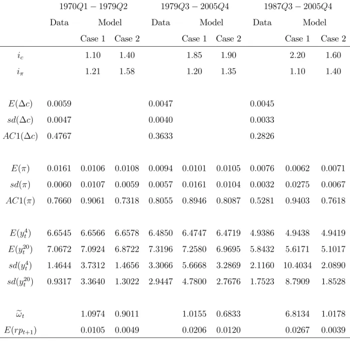
lead to di¤erent pro…les of the term structure of interest rates in various historical periods. Because in‡ation can be endogenously determined through a monetary policy rule in a long-run risk model, this framework provides a venue to explore how changes to monetary policy a¤ect the nominal term structure and whether these e¤ects are consistent with the data for each policy regime. Consequently, a few calibration exercises are conducted using the data from three historical periods which roughly correspond to the terms of several Federal Reserve Board Chairmen. These periods are Burns-Miller (1970:1 to 1979:2), Volcker-Greenspan (1979:3 to 2005:4) and Greenspan-only (1987:3 to 2005:4).
Table 8 and 9 report calibration results for di¤erent periods using Model F and C,
respec-6Some authors do not agree with this view. For example, Orphanides (2004) suggests that the great
in‡ation in the 1970s was the consequence of excessive activist policy response to real economic activity rather than weak policy stance on price stability. Canova and Gambetti (2009) argue that the same policy rule dominated for several decades and their analysis does not support a more aggressive policy in …ghting in‡ation in the Volcker-Greenspan era.
tively. The …rst calibration strategy is to match the level and the slope of the nominal yield curve given consumption dynamics, which is exactly the same method used for the baseline calibration. This is denoted Case 1 in Table 8 and 9. The results show that the Fed’s re-action to macroeconomic activity increased from ic = 1:10 in Burns-Miller to ic = 2:20 in
Greenspan-only. Since the data indicate that consumption growth became lower and less volatile in recent decades, the model suggests that the Fed reduced macroeconomic ‡uctua-tions by adjusting the short rate in a countercyclical manner. In contrast, the Fed’s response to in‡ation was not very di¤erent among these periods, though the coe¢ cient is somewhat larger in Burns-Miller (i = 1:25 in Model F and i = 1:21 in Model C) while relatively smaller during Greenspan-only (i = 1:10 in both Model F and C). Thus the model counter-factually implies that a more proactive stance of price stability is associated with a regime of high and volatile in‡ation in the 1970s. In addition, the volatilities of in‡ation and nom-inal yields predicted by the model are obviously too high, especially in the Greenspan-only period.
Because Case 1 calibration has di¢ culty matching variations of in‡ation and nominal yields, another strategy is to match the volatility of the nominal yields given the consumption dynamics. This is denoted Case 2. The results show that a more aggressive attitude of the Fed in controlling in‡ation is necessary to produce the volatility of nominal yields in the data. As a result, the ‡uctuations of in‡ation are also much lower compared to those in Case 1. However, it is also clear that Case 2 calibration fails to match the slope of the yield curve. More explicitly, nominal rates at the long end are substantially underestimated in all sub-sample periods. For example, the average …ve-year rate was 5:84% in the era of Chairman Greenspan while Model F simply gives a 5:08% …ve-year yield and Model C produces 5:10%. In addition, the model still suggests excessive volatile in‡ation during the terms of Chairman Volcker and Greenspan.
Compared with the literature, these calibration results suggest a quite di¤erent pattern of monetary policy in the postwar United States. Meanwhile, the changes of the term structure in response to the monetary policy shifts are also inconsistent with the data in several aspects. The …rst discrepancy involves the change of policy response to in‡ation from Burns-Miller to Volcker-Greenspan. A strand of research suggests that, if there was a structural change
in the U.S. monetary policy rule in the early 1980s, the conduct of monetary policy was more e¤ective in controlling in‡ation after that time. However, the sub-sample calibration exercises imply a slightly less aggressive attitude toward price stability by the Fed after the 1980s. This discrepancy may be explained by the structure of the model. Since in‡ation is endogenously determined through a monetary policy rule, a more aggressive response to the change of price level lowers the volatility of in‡ation, and the channel of nominal bond pricing also leads to more stable nominal yields. Table 8 and 9 clearly show that more stable in‡ation and nominal yields are associated with a stronger policy stance on controlling in‡ation. However, the macroeconomic data reveal that stable interest rates were associated with volatile in‡ation in Burns-Miller while volatile rates were associated with stable in‡ation in Greenspan-only. To match the volatile interest rates after the 1980s, the policy attitude toward price stability has to be passive so that the model can generate a volatile process of in‡ation. As a result, the model implies that i is on average larger in the 1970s and smaller after the 1980s, which is di¤erent from the pattern suggested in the literature.
The second conundrum concerns the change in the policy response to controlling in‡ation on the term spread. Table 8 and 9 show that i = 1:25 in Burns-Miller corresponds to a 0:38%spread between the …ve-year and one-year yields, and i = 1:20 in Volcker-Greenspan is associated with a 0:83% spread. Thus the model suggests that a more aggressive response to in‡ation shrinks the term spread. Because equilibrium in‡ation is driven by monetary policy in the model, investors believe that a stronger stance on price stability ultimately leads to lower and less volatile in‡ation. As a result, long-term bonds are exposed to less in‡ation risk, and a lower risk premium implies a smaller term spread. However, the spread between the …ve-year and one-year rates in the CRSP Fama-Bliss …le is 0:41% in Burns-Miller, 0:83% in Volcker-Greenspan and 0:90% in Greenspan-only. If monetary policy was more aggressive in controlling in‡ation after the 1980s, a larger i should be associated with a smaller slope of the yield curve. Thus the relationship between the disin‡ation policy and the term spread implied by the model seems not consistent with the data.
Ang, Boivin, Dong and Loo-Kung (2009) argue that a surprise increase in the Fed’s response to in‡ation has a larger e¤ect on the long end of the yield curve. Their impulse response analysis shows that such a policy shift raises the …ve-year yield almost twice as much
as the short rate, and even a small increase in in‡ation loading leads to a sharp increase in the risk premium on long-term bonds. Thus the authors conclude that a stronger stance on price stability during the Volcker-Greenspan period carries a positive price of risk. More explicitly, an unexpected increase in the Fed’s response to in‡ation exposes the entire yield curve to higher in‡ation risk and increases the term spread. This argument seems appealing at …rst glance given that the …ve-year term spread is clearly larger on average in Volcker-Greenspan, and many studies suggest a strong intention to suppress in‡ation during that time. However, there is ample evidence that volatilities of many macroeconomic variables and compensations for various sources of uncertainties, including in‡ation risk, are signi…cantly lower after the mid-1980s. Therefore, it is not clear if a sharp increase in the short rate target should be interpreted as introducing more in‡ation risk on long-term bonds.
Palomino (2012) also …nds it di¢ cult to reconcile the increasing average term spread with the improved credibility of monetary policy from the 1950s to the early 2000s. His analysis also shows that the higher credibility of monetary policy during the Bretton Woods regime accounts for a smaller term spread on average. However, the larger average term spread in the Greenspan era cannot be rationalized by the same story. Palomino suggests that one possible interpretation of this phenomenon could be a suspicion in the policy credibility improvements in the Greenspan era. Although monetary policy is believed to have been more aggressive in controlling in‡ation during the Volcker-Greenspan period, the Fed did not explicitly state a nominal anchor. Hence an essentially lower credibility of monetary policy is not out of the question given that the public may not understand the policy well. On the other hand, other factors that are not related to monetary policy could also be a reason. The model cannot account for these factors if we do not know what they are and how they a¤ect the term structure of interest rates. In sum, providing a coherent explanation for the relatively large term spread in the quiescent Volcker-Greenspan period continues to be challenging.
The third problem focuses on the magnitude of the policy response to in‡ation and consumption growth. To reproduce the positive slope of the nominal yield curve, the model imposes the restriction i > 1 and disciplines ic to be positive and su¢ ciently large. The
stationary equilibrium. The empirical work by Orphanides (2004) suggests a similarly strong policy reaction to in‡ation, i.e., i > 1, in the pre- and post-Volcker periods. However, most other studies of postwar U.S. monetary policy do not suggest that the Fed always adhered to the Taylor principle. Clarida, Galí and Gertler (2000) apply the generalized method of moments (GMM) to estimate a simple forward-looking monetary policy rule similar to (8). Their baseline estimate of i is 2:15 for the Volcker-Greenspan era while the estimate for the pre-Volcker period is merely 0:68. Their estimates of ic are much smaller than i and
are statistically insigni…cant for the Volcker-Greenspan era. In addition, the estimates of policy responses to in‡ation and output gap are quite divergent in the literature. Ang, Dong and Piazzesi (2007) use a no-arbitrage pricing technique to estimate various speci…cations of the Taylor rule for the period June 1952 to December 2004. Their benchmark estimates are ic = 0:509 and i = 0:238 for a contemporaneous rule and ic = 0:590and i = 0:292 for
a forward-looking rule. In sum, these studies are far from unanimous on the Fed’s stance of price and output stability, and few of them support the prevailing aggressive policy in the past decades.
In addition to the above problems, the inconsistency between Euler equation interest rates and money market rates seems to be a more fundamental challenge. To clear the bond market, the short rate implied by the Euler equation has to equal the target rate set by the Fed. This condition not only determines the equilibrium in‡ation but also illuminates the e¤ects of monetary policy on the term structure of interest rates. However, Canzoneri, Cumby and Diba (2007) …nd that the behavior of the Federal Funds rate is quite di¤erent from the short rate implied by many asset pricing models. Their analysis shows that the gap between the two rates links to the stance of monetary policy. More explicitly, a tightening policy increases the money market rate and reduces the Euler equation rate. Thus the correlation of the Euler equation rate and the money market rate is systematically negative, which casts doubt on the equivalence of the two rates in many asset pricing as well as macroeconomic models.
Unfortunately, the long-run risk model with endogenous in‡ation is not immune to this critique. The Euler equation rate from the model, which is the right-hand side of (11), can
be expressed as ( 0 m0) 1 2 (mw w) 2 + 2 + ( x mx) xt+ uut + ( m ) 1 2 (m ) 2 + (m )2 2t: (22) Given that u < 0, it is clear that a positive monetary policy shock decreases the Euler
equation rate. On the other hand, the positive values of ic and i imply an increase in
the money market rate in response to the same shock. Thus the model is not free from this inconsistency problem. If we address this issue by calibrating a positive u, the model
will not be able to account for some stylized facts of the term structure and in‡ation. For example, u > 0 leads to a counterfactually downward-sloping nominal yield curve and also
erroneously implies that an aggressive disin‡ation policy ampli…es the volatility of in‡ation.
5
Conclusion
Because in‡ation is not structural in most consumption-based asset pricing models, it is di¢ cult to explore how in‡ation drivers a¤ect the dynamics of nominal yields. To address this issue, I augment a baseline long-run risk model with a monetary policy rule so that the equilibrium process for in‡ation is endogenously determined. Calibration with postwar U.S. data suggests that, given the aggressive monetary policy responses to in‡ation and economic growth, the model captures the negative correlation of in‡ation and consumption growth in the data. This implies positive risk premia carried by nominal bonds and the average upward-sloping nominal term structure of interest rates. The decomposition of nominal SDF also shows that the risk premia implied by the model with endogenous in‡ation are much closer to the empirical estimates than those implied by the model with exogenous in‡ation. However, calibration exercises for three historical periods indicate some discrepancies between the model and the data. The model implies that a passive monetary policy is associated with volatile nominal yields and a large term spread in the era of Chairmen Volcker and Greenspan, while many studies suggest that the conduct of monetary policy essentially shows a stronger stance on price stability during that period. Meanwhile, the model requires the policy rule coe¢ cients on in‡ation and economic growth to exceed unity to account for the positive
slope of the term structure. Unfortunately, it seems that this condition lacks empirical support. Last but not least, the model is not free from the fundamental problem that the Euler equation and money market rates are not consistent.
The model developed in this paper does not allow any feedback from in‡ation to con-sumption growth. In some recent studies, a production economy with investment wedges or sticky prices can endogenously generate long-run risk. This framework is able to incorporate complicated interplays among in‡ation and other real variables. For example, Gavazzoni (2012) shows that long-run risk arises in a New Keynesian model with recursive preference and monetary policy inertia. This approach addresses the non-neutrality of in‡ation, but the calibration in Gavazzoni (2012) implies a counterfactually downward-sloping nominal term structure. On the other hand, the inconsistency between the Euler equation and money market rates also attracts more attention. Collard and Dellas (2012) show that a prefer-ence with non-separability between leisure and consumption partially improves the model …t. However, this strategy does not eradicate the inconsistency problem. The solutions to these problems are left for future research.
6
Appendix
6.1
Model Solution
To solve for the model, …rst plug equation (9) and (10) into (2). The real SDF can be expressed as follows: mt+1= m0+ mxxt+ m t2+ m t t+1+ m t t+1+ mwwt+1; (23) mx = 1 ; (24) m = (1 )A2(1 1 1); (25) m = ; (26) m = (1 ) 1A1'e; (27) mw = (1 ) 1A2 w; (28) m0 = ln (1 ) 0+ (1 )(1 1)A0 (1 ) 1A2(1 1) 2; (29)
where 0, 1, A0, A1 and A2 are the same as those in Bansal and Yaron (2004): 1 = exp (z) 1 + exp (z); (30) 0 = ln [1 + exp (z)] 1z; (31) A1 = 1 1= 1 1 ; (32) A2 = [(1 )2+ ( A 1 1'e)2] 2 (1 1 1) ; (33) A0 = 1 1 1 ln + 1 1 + 0+ 1A2(1 1) 2+ 1 2 ( 1A2 w) 2 : (34)
Plug (23) and the conjectured process for in‡ation (12) or (13) gives the expression of mt+1 t+1, which is the nominal SDF. Thus the equilibrium process for in‡ation is solved
by plugging nominal SDF into (11). For Model F (forward-looking policy rule), the associated coe¢ cients are
x = mx+ ic (1 i ); (35) = 1 1(1 i ) m + 1 2 m 2+ (m x'e) 2 ; (36)
u = 1 u(1 i ) ; (37) 0 = 1 1 i m0 (1 i )(1 1) 2+1 2(mw w) 2 2 u 2+ i 0+ ic : (38)
For Model C (contemporaneous rule), the associated coe¢ cients are
x = ic+ mx i ; (39) = 1 1 i m + 1 2 1 (m ) 2 + (m )2 ; (40) u = u u i ; (41) = ic i ; (42) = 'e( x mx) i ; (43) w = 1 i m 1 2 w (m ) 2 + (m )2 ; (44) = ( u 1) i ; (45) 0 = 1 1 i m0+ i0+ ic + 1 2 (mw w) 2+ 2 + 2(1 1) 1 i m + 1 2(m ) 2 + 1 2(m ) 2 ; (46) To solve for equilibrium nominal bond prices, plug the expression of nominal SDF and (16) into (15). For Model F, the coe¢ cients are
e Bxn = mx x Bexn 1 ; (47) e Bn= m 1 Ben 1 + 1 2 m 2+hm ' e x Bexn 1 i2 ; (48) e Bun= u u Beun 1 ; (49) e B0n = m0 0 Be0n 1 Be n 1 (1 1) 2 +1 2 h mw w Ben 1 i2 +1 2 2 u Beun 1 2 : (50)
For Model C, the coe¢ cients are e Bxn= mx x+ Bexn 1; (51) e Bn= m + 1Ben 1+ 1 2 (m ) 2 + m + 'eBexn 1 2 ; (52) e Bun= u + uBeun 1; (53) e B0n = m0 0+ eB0n 1+ eB n 1(1 1) 2 +1 2 mw w + wBe n 1 2+ Ben 1 u 2 : (54)
The associated nominal yields can be derived using (17).
6.2
Decompose the SDF
According to Alvarez and Jermann (2005), the transitory component of the nominal SDF can be obtained by e NT t+1 e NT t = lim n !1e exp ep n t pe n 1 t+1 ; (55)
where e is a number. For Model F, we can infer that e Bx1= mx x 1 ; (56) e Bu1= u u 1 u; (57) e B1 = 1 1 1 m 1 + 1 2m 2 +1 2 h m 'e x Bex1 i2 : (58) Thus the transitory component of the nominal SDF becomes
e Nt+1T e NT t = e expf(1 ) eBx1xt+ (1 1) 2t 2 Be1 + (1 u) eB1u ut 'eBe1x t t+1 Be1 wwt+1 Beu1 t+1g: (59)
Since the limit of eB0n 1 Ben
0 is …nite, the constant e is chosen to o¤set this term as n grows:
e = exph lim n !1 Be n 0 Be n 1 0 i : (60)
The martingale component is then de…ned as e NP t+1 e NP t = Net+1 e Nt e NT t+1 e NT t ! 1 : (61)
Some algebras lead to the following result: e mPt+1 = 1 2 m 2 +hm ' e x Bex1 i2 2 t + m t t+1 +hm 'e x Bex1 i t t+1+ h mw w Be1 i wt+1 + Beu1 u t+1 1 2 h mw w Be1 i2 1 2 h u Beu1 i2 : (62)
Thus the ratio of the conditional variance of the martingale component to the conditional variance of the whole SDF is
e !t= m2 +hm ' e x Bex1 i2 2 t + h mw w Be1 i2 +h u Beu1 i2 m2 + (m ' e x) 2 2 t + (mw w ) 2 + 2 2 u : (63) For Model C, the same procedure is implemented and the associated conditional variance ratio is: e !t = (m )2+ m + 'eBex1 2 2 t + mw w+ wBe1 2 + Beu1 2 (m )2+ (m )2 2 t + (mw w)2+ 2 : (64) This completes the decomposition of the volatility of the SDF for both model speci…cations.
References
[1] Alvarez, Fernando and Urban J. Jermann, 2005, Using Asset Prices to Measure the Persistence of the Marginal Utility of Wealth, Econometrica, 73: 1977-2016.
[2] Ang, Andrew, Jean Boivin, Sen Dong, and Rudy Loo-Kung, 2011, Monetary Policy Shifts and the Term Structure, Review of Economic Studies, 78: 429-457.
[3] Ang, Andrew, Sen Dong and Monika Piazzesi, 2007, No-Arbitrage Taylor Rules, Work-ing Paper.
[4] Bansal, Ravi and Ivan Shaliastovich, 2008, A Long-Run Risks Explanation of Pre-dictability Puzzles in Bond and Currency Markets, Working Paper.
[5] Bansal, Ravi and Amir Yaron, 2004, Risks for the Long Run: A Potential Resolution of Asset Pricing Puzzles, Journal of Finance, 59: 1481-1509.
[6] Canzoneri, Matthew, Robert Cumby and Behzad Diba, 2007, Euler Equations and Money Market Interest Rates: A Challenge for Monetary Policy Models, Journal of Monetary Economics, 54: 1863–1881.
[7] Canova, Fabio and Luca Gambetti, 2009, Structural Changes in the US Economy: Is There a Role for Monetary Policy? Journal of Economic Dynamics and Control, 32: 477-490.
[8] Clarida, Richard, Jordi Galí and Mark Gertler, 2000, Monetary Policy Rule and Macro-economic Stability: Evidence and Some Theory, Quarterly Journal of Economics, 115: 147–180.
[9] Cogley, Timothy and Thomas Sargent, 2001, Evolving Post-World War II U.S. In‡ation Dynamics, NBER Macroeconomic Annual, 16: 331–373.
[10] Cogley, Timothy and Thomas Sargent, 2005, Drifts and Volatilities: Monetary Policies and Outcomes in the Post WWII U.S., Review of Economic Dynamics, 8: 262–302.
[11] Collard, Fabrice and Harris Dellas, 2012, Euler equations and monetary policy, Eco-nomics Letters, 114: 1-5.
[12] Dittmar, Robert and Francisco Palomino, 2010, Long Run Labor Income Risk, Working Paper.
[13] Doh, Taeyoung, 2011, Long Run Risks in the Term Structure of Interest Rates: Esti-mation, Journal of Applied Econometrics, forthcoming.
[14] Epstein, Larry and Stanley Zin, 1989, Substitution, Risk Aversion, and the Temporal Behavior of Consumption and Asset Returns: a Theoretical Framework, Econometrica, 57: 937-969.
[15] Eraker, Bjørn, Ivan Shaliastovich and Wenyu Wang, 2011, Durable Goods, In‡ation Risk and the Equilibrium Term Structure, Working Paper.
[16] Gallmeyer, Michael, Burton Holli…eld, Francisco Palomino and Stanley Zin, 2007, Arbi-trage Free Bond Pricing with Dynamic Macroeconomic Models, Federal Reserve Bank of St. Louis Review, 89: 305-326.
[17] Gallmeyer, Michael, Burton Holli…eld, Francisco Palomino and Stanley Zin, 2009, Term Premium Dynamics and the Taylor Rule, Working Paper.
[18] Gavazzoni, Federico, 2012, Nominal Frictions, Monetary Policy and Long-Run Risk, Working Paper.
[19] Hasseltoft, Hanrik, 2012, Stocks, Bonds, and Long-Run Consumption Risks, Journal of Financial and Quantitative Analysis, 47: 309-332.
[20] Koijen, Ralph, Hanno Lustig, Stijn Van Nieuwerburgh and Adrien Verdelhan, 2010, Long-Run Risk, the Wealth-Consumption Ratio, and the Temporal Pricing of Risk, American Economic Review, 100: 552-556.
[21] Lubik, Thomas and Frank Schorfheide, 2004, Testing for Indeterminacy: An Application to US Monetary Policy, American Economic Review, 94: 190–217.
[22] Orphanides, Athanasios, 2004, Monetary Policy Rules, Macroeconomic Stability, and In‡ation: A View from the Trenches, Journal of Money, Banking and Credit, 36: 151-175.
[23] Palomino, Francisco, 2012, Bond Risk Premiums and Optimal Monetary Policy, Review of Economic Dynamics, 15: 19-40.
[24] Piazzesi, Monika and Martin Schneider, 2007, Equilibrium Yield Curves, NBER Macro-economics Annual, 21: 389-442.
[25] Restoy, Fernando and Phillippe Weil, 2011, Approximate Equilibrium Asset Prices, Review of Finance, 15: 1-28.
[26] Shiller, Robert, 1979, The Volatility of Long-Term Interest Rates and Expectations Models of the Term Structure, Journal of Political Economy, 87: 1190-1219.
[27] Yang, Wei, 2011, Long-Run Risk in Durable Consumption, Journal of Financial Eco-nomics, 102: 45-61.
Common Parameters Forward-Looking Rule Contemporaneous Rule 0:0049 i0 0:00518 i0 0:00532 0:9671 ic 1:5 ic 1:5 0:0034 i 1:35 i 1:35 'e 0:2447 u 0:99 u 0:99 1 0:9771 2:5 10 4 2:5 10 4 w 0:02 10 5 0:998 7:5 1:5
Table 1: Calibrated Parameter Values
Data Model F Model C E( c) 0:0049 0:0049 0:0049 sd( c) 0:0048 0:0047 0:0047 AC1( c) 0:4648 0:4648 0:4648 E( ) 0:0089 0:0076 0:0077 sd( ) 0:0064 0:0095 0:0096 AC1( ) 0:7957 0:9737 0:8340 corr( c; ) 0:1073 0:1762 0:2593
Table 2: Moments of Consumption Growth and In‡ation
This table reports some moments of consumption dynamics and in‡ation. "Model F" means model with forward-looking policy rule, "Model C" means model with contemporaneous policy rule, "AC1" means the …rst-order correlation coe¢ cient and "corr" means linear correlation coe¢ cient.
Model F i 1:2 1:5 1:8 2:2 E( ) 0:0146 0:0051 0:0031 0:0020 sd( ) 0:0167 0:0067 0:0042 0:0028 Model C i 1:2 1:5 1:8 2:2 E( ) 0:0145 0:0052 0:0032 0:0021 sd( ) 0:0155 0:0072 0:0049 0:0036
Table 3: The Stance of Monetary Policy and Equilibrium In‡ation
This table shows the mean and the standard deviation of in‡ation with di¤erent values of i .
1-year 2-year 3-year 4-year 5-year Data 5:2392 5:4386 5:6156 5:7560 5:8545 (3:0168) (2:9755) (2:8944) (2:8473) (2:7823) Model F 5:2485 5:4253 5:5835 5:7252 5:8525 (3:0773) (2:9515) (2:8356) (2:7285) (2:6294) Model C 5:2523 5:4153 5:5614 5:6925 5:8103 (2:8834) (2:7684) (2:6623) (2:5642) (2:4734)
Table 4: The Level and Volatility of Nominal Yields
The average levels of nominal yields are reported in the …rst line of each panel, and the associated volatilities are reported in the parentheses. All values are reported in per annum percentage points. "Data" comes from the CRSP Fama-Bliss …le and only maturities of one through …ve years are available.
1-year 2-year 3-year 4-year 5-year Data 3:0168 2:9755 2:8944 2:8473 2:7823 u = 0:99 3:0773 2:9515 2:8356 2:7285 2:6294 u = 0:95 2:4376 2:2788 2:1342 2:0024 1:8820 u = 0:50 2:2737 2:1309 2:0026 1:8850 1:7769 u = 0:10 2:2685 2:1287 2:0011 1:8839 1:7759
Table 5: Volatilities of Nominal Yields and the Persistence of Monetary Policy Shock: Model F
The table exhibits the volatilities of nominal yields with di¤erent persistence of monetary policy shock implied by the model. The monetary policy is described by a forward-looking rule. All values are reported in per annum percentage points.
1-year 2-year 3-year 4-year 5-year Data 3:0168 2:9755 2:8944 2:8473 2:7823
u = 0:99 2:8834 2:7684 2:6623 2:5642 2:4734 u = 0:95 2:2022 2:0598 1:9300 1:8115 1:7032
u = 0:50 2:0734 1:9462 1:8294 1:7220 1:6232 u = 0:10 2:0732 1:9461 1:8293 1:7220 1:6231
Table 6: Volatilities of Nominal Yields and the Persistence of Monetary Policy Shock: Model C
The table exhibits the volatilities of nominal yields with di¤erent persistence of monetary policy shock implied by the model. The monetary policy is described by a contemporaneous rule. All values are reported in per annum percentage points.
1-year 2-year 3-year 4-year 5-year Data 0:35 0:55 0:73 0:87 0:97
BS 0:33 0:93 1:59 2:27 2:97 Model F 0:37 0:69 0:97 1:22 1:43 Model C 0:34 0:64 0:91 1:14 1:34
Table 7: Nominal Bond Risk Premium
The table reports the average nominal bond risk premium per annum. BS means Bansal and Shaliastovich (2008), calculated by Koijen et al. (2010).
1970Q1 1979Q2 1979Q3 2005Q4 1987Q3 2005Q4
Data Model Data Model Data Model Case 1 Case 2 Case 1 Case 2 Case 1 Case 2 ic 1:10 1:42 1:80 1:80 2:20 1:50 i 1:25 1:60 1:20 1:35 1:10 1:40 E( c) 0:0059 0:0047 0:0045 sd( c) 0:0047 0:0040 0:0033 AC1( c) 0:4767 0:3633 0:2826 E( ) 0:0161 0:0105 0:0107 0:0094 0:0100 0:0105 0:0076 0:0059 0:0071 sd( ) 0:0060 0:0093 0:0052 0:0057 0:0168 0:0096 0:0032 0:0337 0:0059 AC1( ) 0:7660 0:9806 0:9745 0:8055 0:9736 0:9736 0:5281 0:9736 0:9802 E(yt4) 6:6545 6:6492 6:6566 6:4850 6:4899 6:4821 4:9386 4:9770 4:9377 E(y20 t ) 7:0672 7:0302 6:8841 7:3196 7:3231 6:9677 5:8432 5:6235 5:0830 sd(yt4) 1:4644 3:3117 1:4749 3:3066 6:1838 3:3070 2:1160 13:0029 2:0976 sd(y20 t ) 0:9317 2:9855 1:3067 2:9447 5:1991 2:7969 1:7523 10:8126 1:8734 e !t 1:0454 0:8944 1:1025 0:7190 9:8078 1:0769 E(rpt+1) 0:0092 0:0051 0:0226 0:0118 0:0346 0:0036
Table 8: Experiments on In‡ation Response: Model F
The table presents calibration exercises for Model F with some sub-sample periods. The moments of nominal yields are reported in per annum percentage points.
1970Q1 1979Q2 1979Q3 2005Q4 1987Q3 2005Q4
Data Model Data Model Data Model Case 1 Case 2 Case 1 Case 2 Case 1 Case 2 ic 1:10 1:40 1:85 1:90 2:20 1:60 i 1:21 1:58 1:20 1:35 1:10 1:40 E( c) 0:0059 0:0047 0:0045 sd( c) 0:0047 0:0040 0:0033 AC1( c) 0:4767 0:3633 0:2826 E( ) 0:0161 0:0106 0:0108 0:0094 0:0101 0:0105 0:0076 0:0062 0:0071 sd( ) 0:0060 0:0107 0:0059 0:0057 0:0161 0:0104 0:0032 0:0275 0:0067 AC1( ) 0:7660 0:9061 0:7318 0:8055 0:8946 0:8087 0:5281 0:9403 0:7618 E(yt4) 6:6545 6:6566 6:6578 6:4850 6:4747 6:4719 4:9386 4:9438 4:9419 E(y20 t ) 7:0672 7:0924 6:8722 7:3196 7:2580 6:9695 5:8432 5:6171 5:1017 sd(yt4) 1:4644 3:7312 1:4656 3:3066 5:6668 3:2869 2:1160 10:4034 2:0890 sd(y20 t ) 0:9317 3:3640 1:3022 2:9447 4:7800 2:7676 1:7523 8:7909 1:8528 e !t 1:0974 0:9011 1:0155 0:6833 6:8134 1:0178 E(rpt+1) 0:0105 0:0049 0:0206 0:0120 0:0267 0:0039
Table 9: Experiments on In‡ation Response: Model C
The table presents calibration exercises for Model C with some sub-sample periods. The moments of nominal yields are reported in per annum percentage points.
國科會補助專題研究計畫出席國際學術會議心得報告
日期: 102 年 5 月 29 日
一、參加會議經過
個人於 102/5/16 搭乘班機經日本東京與美國芝加哥兩度轉機,於當日晚間抵達會
議地點伊利諾州香檳市(Champaign, IL)。5/17 與 5/18 兩日均於伊利諾大學香檳
分校(UIUC)經濟系參與此次 Midwest Macro 年度研討會,個人的論文發表則 安排於 5/18 下午的場次,同時並擔任該場次主持人。此次會議於 5/19 上午雖仍 有議程,然考量個人服務單位之教學問題,只能於當日早晨先行離席返國,結束 此次會議行程。
二、與會心得
本研討會近年來成為美國總體經濟學界重要的交流場合,一些先進的總體理論、 實證與政策分析論文皆能在會議中看到。論文發表者除美國知名大學的年輕學者 外,亦有不少各國中央銀行(U.S. Fed, Bank of Canada, Bank de France 等)的研 究人員參與,個人就與同場次一位服務於 Fed Board 的研究人員交流了一些有關 利率期限結構與貨幣政策議題的意見,收穫不少。議程中亦有不少關於政策不確 定性(policy uncertainties)與零利率(zero lower bound)貨幣政策的影響分析, 對於個人未來的研究思路有所啟發。主辦單位於議程中安排了兩場 plenary speech,分別是 5/17 晚間 UCLA 的 Lee Ohnian 教授主講 The Decline of the Rust Band,以及 5/18 晚間 University of Minnesota 的 Victor Rios-Rull 教授主講 A New View of Cyclical Movements in Productivity。前者的本質是一個美國經濟史的議 題,但 Ohnian 教授卻能以現代總體模型解釋五大湖區自二次大戰後產業蕭條的計畫編號 NSC101-2410-H-004-028-
計畫名稱 以長期風險模型結合貨幣政策探究利率的期限結構
出國人員
姓名
趙世偉
服務機構
及職稱
國立政治大學金融學系
會議時間 102/5/16~102/5/19
會議地點 Champaign, IL, USA
會議名稱 Midwest Macroeconomics Meetings 2013
發表題目
Long Run Risks, Monetary Policy and the Term Structure of
Interest Rates
原因:該地區的高工資與缺乏競爭,令人見識到其總體經濟分析的功力。後者則 是對景氣波動的新解,Rios-Rull 教授認為許多看似為生產(供給)面的現象其 實是來自需求面,因為 search frictions 的存在使得來自需求面的衝擊(例如: preference shock)在現代總體模型中看來像是供給面衝擊。此種觀點與近幾十年 來的總體經濟理論發展有相當大的出入,目前尚難論定此說的可信度,但這項研 究確實提供了許多新穎的思考方向,值得進一步分析探究。總之,個人在數天的 議程中確實見識到不少值得深思的總體經濟議題與研究方法。
三、發表論文全文或摘要
論文摘要:Many previous studies of the term structure of interest rates specify the process for inflation exogenously. Because monetary policy is a crucial driver of inflation, this paper attempts to endogenize the process for inflation through a monetary policy rule and examines the performance of the model. Calibration results suggest that, given the strong stance of monetary policy, the model is able to explain the average upward-sloping nominal yield curve, volatile long rates and the downward-sloping term structure of volatility. The decomposition of the nominal stochastic discount factor in the manner of Alvarez and Jermann (2005) also suggests that the negative correlation of equilibrium inflation and the monetary policy shock help to match the risk premium in the data. However, the model has difficulty connecting the monetary policy and the term structure of interest rates across different regimes.
四、攜回資料名稱及內容
攜回資料為本次會議之議程與發表論文一覽表。
五、其它
國科會補助計畫衍生研發成果推廣資料表
日期:2013/08/16國科會補助計畫
計畫名稱: 以長期風險模型結合貨幣政策探究利率的期限結構 計畫主持人: 趙世偉 計畫編號: 101-2410-H-004-028- 學門領域: 財務經濟學無研發成果推廣資料
101 年度專題研究計畫研究成果彙整表
計畫主持人:趙世偉 計畫編號: 101-2410-H-004-028-計畫名稱:以長期風險模型結合貨幣政策探究利率的期限結構 量化 成果項目 實際已達成 數(被接受 或已發表) 預期總達成 數(含實際已 達成數) 本計畫實 際貢獻百 分比 單位 備 註 ( 質 化 說 明:如 數 個 計 畫 共 同 成 果、成 果 列 為 該 期 刊 之 封 面 故 事 ... 等) 期刊論文 0 0 100% 研究報告/技術報告 0 0 100% 研討會論文 0 0 100% 篇 論文著作 專書 0 0 100% 申請中件數 0 0 100% 專利 已獲得件數 0 0 100% 件 件數 0 0 100% 件 技術移轉 權利金 0 0 100% 千元 碩士生 0 0 100% 博士生 1 1 100% 博士後研究員 0 0 100% 國內 參與計畫人力 (本國籍) 專任助理 0 0 100% 人次 期刊論文 0 0 100% 研究報告/技術報告 0 0 100% 研討會論文 1 1 100% 篇 論文著作 專書 0 0 100% 章/本 申請中件數 0 0 100% 專利 已獲得件數 0 0 100% 件 件數 0 0 100% 件 技術移轉 權利金 0 0 100% 千元 碩士生 0 0 100% 博士生 0 0 100% 博士後研究員 0 0 100% 國外 參與計畫人力 (外國籍) 專任助理 0 0 100% 人次其他成果
(
無法以量化表達之成 果如辦理學術活動、獲 得獎項、重要國際合 作、研究成果國際影響 力及其他協助產業技 術發展之具體效益事 項等,請以文字敘述填 列。) 無 成果項目 量化 名稱或內容性質簡述 測驗工具(含質性與量性) 0 課程/模組 0 電腦及網路系統或工具 0 教材 0 舉辦之活動/競賽 0 研討會/工作坊 0 電子報、網站 0 科 教 處 計 畫 加 填 項 目 計畫成果推廣之參與(閱聽)人數 0國科會補助專題研究計畫成果報告自評表
請就研究內容與原計畫相符程度、達成預期目標情況、研究成果之學術或應用價
值(簡要敘述成果所代表之意義、價值、影響或進一步發展之可能性)
、是否適
合在學術期刊發表或申請專利、主要發現或其他有關價值等,作一綜合評估。
1. 請就研究內容與原計畫相符程度、達成預期目標情況作一綜合評估
■達成目標
□未達成目標(請說明,以 100 字為限)
□實驗失敗
□因故實驗中斷
□其他原因
說明:
2. 研究成果在學術期刊發表或申請專利等情形:
論文:□已發表 □未發表之文稿 ■撰寫中 □無
專利:□已獲得 □申請中 ■無
技轉:□已技轉 □洽談中 ■無
其他:(以 100 字為限)
3. 請依學術成就、技術創新、社會影響等方面,評估研究成果之學術或應用價
值(簡要敘述成果所代表之意義、價值、影響或進一步發展之可能性)(以
500 字為限)
This research sheds some light on the importance of monetary policy for an asset pricing model to jointly capture asset returns, risks and macroeconomic variables. Even if the model characterizes an endowment economy, endogenous process for inflation still substantially improves its performance. This model addresses how long run risks and monetary policy jointly determine the term structure of interest rates. The decomposition of the nominal stochastic discount factor in the manner of Alvarez and Jermann (2005) also suggests that the negative correlation of equilibrium inflation and the monetary policy shock help to match the risk premium in the data. This framework may deserve more future work since it still has difficulty describing inflation and the term structure of yields across different historical regimes.