A context adaptive bit-plane coder with maximum-likelihood-based stochastic bit-reshuffling technique for scalable video coding

A Context Adaptive Bit-Plane Coder With

Maximum-Likelihood-Based Stochastic

Bit-Reshuffling Technique for Scalable Video Coding

Wen-Hsiao Peng, Tihao Chiang, Senior Member, IEEE, Hsueh-Ming Hang, Fellow, IEEE, and

Chen-Yi Lee, Member, IEEE

Abstract—In this paper, we propose a context adaptive bit-plane coding (CABIC) with a stochastic bit reshuffling (SBR) scheme to deliver higher coding efficiency and better subjective quality for fine granular scalable (FGS) video coding. Traditional bit-plane coding in FGS algorithm suffers from poor coding efficiency and subjective quality. To improve coding efficiency, our CABIC constructs context models based on both the energy distribution in a block and the spatial correlations in the adjacent blocks. Moreover, it exploits the context across bit-planes to save side information. To improve subjective quality, our SBR reorders the coefficient bits by their estimated rate-distortion performance. Particularly, we model transform coefficients with Laplacian distributions and incorporate them into the context probability models for content-aware parameter estimation. Moreover, our SBR is implemented with a dynamic priority management that uses a low-complexity dynamic memory organization. Experimental results show that our CABIC improves the PSNR by 0.5 1.0 dB at medium and high bit rates. While maintaining similar or even higher coding efficiency, our SBR improves the subjective quality. Index Terms—Bit-plane coding, fine granularity scalability, scalable video coding.

I. INTRODUCTION

S

CALABLE video coding attracts wide attention with the rapid growth of multimedia applications over Internet and wireless channels. In such applications, the video may be trans-mitted over error-prone channels with fluctuated bandwidth. To serve multimedia applications under a heterogeneous environ-ment, MPEG-4 has defined the fine granularity scalability (FGS) [7] that provides a discrete cosine transform (DCT)-based scal-able approach in a layered fashion. Currently, the base layer is coded by a non-scalable codec while the enhancement layer is coded with an embedded bit-plane coding using variable-length code (VLC). While offering FGS, current bit-plane coding poses two major disadvantages.

1) Poor coding efficiency: Poor coding efficiency is con-tributed by three factors. Firstly, information with different weighting is jointly grouped by (Run, EOP) symbols and coded without differentiation. Secondly, the coding of Manuscript received August 20, 2004; revised May 25, 2005. The associate editor coordinating the review of this manuscript and approving it for publica-tion was Dr. Chang Wen Chen.

The authors are with the Department of Electronics Engineering, National Chiao-Tung University, Hsinchu 30010, Taiwan, R.O.C. (e-mail: pawn@mail. si2lab.org; [email protected]; [email protected]; cylee@cc. nctu.edu.tw).

Digital Object Identifier 10.1109/TMM.2006.876302

each bit-plane is independent and the coding of each DCT block is uncorrelated with adjacent neighbors. Existing correlations across bit-planes and among spatially adjacent blocks are not fully exploited. Lastly, the VLC tables have limitations to adapt the statistics for each sequence. 2) Poor subjective quality: Poor subjective quality is caused

by the frame raster scanning. For each bit-plane, the current approach performs the coding in a block-by-block manner. As the enhancement layer is partially decoded, the frame raster scanning may only refine the upper part with one extra bit-plane. Such uneven refinement causes the degra-dation of subjective quality.

In this paper, our goal is to provide a generic bit-plane coding that delivers higher coding efficiency and better subjective quality. Our scheme is useful not only for MPEG-4 FGS [7], but also for the advanced FGS algorithms, [3], [4], [9], [12], [15].

For improving the coding efficiency, our prior work [10] has shown that simply replacing VLC with arithmetic coding is in-sufficient unless efficient context model are used. The existing approaches, [5], [8], have taken the context adaptive bit-plane coding (CABIC) for the DCT-based image coding. Specifically, the transform coefficients are first partitioned into significant bits and refinement bits, as in [13]. Then, the context model for each type of bits is designed according to different correlations. In [5], the energy distribution of 8 8 DCT is used to construct a “Run” index for the significant bit. In [8], the spatial correla-tions are considered by referring to the significance status of the adjacent and co-located coefficients as the context model. How-ever, for predictive enhancement-layer coding in the advanced FGS algorithms, [3], [4], [9], [12], [15], using context models of lower order is insufficient because the signal is more like noise. To tackle this problem, our prior work [11] designs context models by jointly considering the energy distribution in a block and the spatial correlations in the adjacent blocks. Moreover, we employ the context across bit-planes to save side information. Although the context models are different, all the schemes try to fully use the existing correlations for better coding efficiency. While the coding efficiency is improved by the CABIC, the poor subjective quality from the frame raster scanning still re-mains. For improving the subjective quality, MPEG-4 FGS [7] offers a frequency weighting tool. The basic idea is to shift up the coefficients of lower frequency so that they can be transmitted first. The subjective quality is improved since the refinement of each block becomes more uniform. However, the shift introduces 1520-9210/$20.00 © 2006 IEEE

redundant bits that decrease the coding efficiency. On the av-erage, at the same bit rate, a PSNR loss of 2 3 dB is observed when the frequency weighting is enabled. To keep high coding ef-ficiency, [1] presents a deterministic, group-based coding order. The transform coefficients in each block are partitioned into several subgroups. The coding of a subgroup can only be started when the previous subgroup of all blocks is finished. Apparently, the deterministic partition is not optimized for every sequence.

To adapt the coding order for different input sequences, dy-namic bit-reshuffling schemes are proposed in our prior work [11] and the work by Li et al. [6]. The idea of bit reshuffling is to dynamically determine the coding order of each bit by its estimated rate-distortion performance. The coefficient bit with better rate-distortion performance is coded with higher priority. In [6], the bit reshuffling was first proposed to provide rate-dis-tortion optimization specifically for the wavelet-based image codec. In [11], it is used to improve the subjective quality of the FGS algorithms. Previous results in [11] show that dynamic bit reshuffling can effectively improve the subjective quality while maintaining similar or even higher coding efficiency.

In this paper, we propose an enhanced stochastic bit-reshuf-fling (SBR) scheme. Instead of using the uniform distribution in [6], we model transform coefficients with discrete Laplacian distributions, which are derived from maximum likelihood prin-ciple. Moreover, we incorporate the context probability models into the discrete Laplacian distributions to estimate the rate-distortion functions of the transform coefficients. Furthermore, to make bit reshuffling content aware so as to improve the sub-jective quality, a dynamic priority management is developed by considering a content dependent priority and a rate-distortion data update mechanism. Since the bit reshuffling requires inten-sive computations, we further propose a dynamic memory or-ganization to reduce complexity. In summary, our contributions and the features of this work include the following.

• A CABIC scheme that constructs context models based on both the energy distribution in a block and the spatial correlations in the adjacent blocks to deliver higher coding efficiency.

• A bit-plane partition scheme that exploits the context across bit-planes to save side information.

• An estimated Laplacian distribution is used for efficient coding of refinement bits.

• A maximum likelihood estimator is used to minimize the overhead for the Laplacian parameters.

• A 4 4 integer transform in [14] is used to avoid the con-text dilution problem.

• A content aware SBR that uses estimated Laplacian distri-butions and context probability models to improve subjec-tive quality.

• A dynamic priority management implemented with a dy-namic memory organization is used for SBR.

Experimental results show that our CABIC provides a PSNR gain of 0.5 1.0 dB over the VLC-based bit-plane coding [7]. While maintaining similar or even higher coding efficiency, our SBR significantly improves the subjective quality.

The rest of this paper is organized as follows: Section II presents the algorithm of CABIC. Section III introduces the concept of SBR. Section IV shows the parameter estimation in

SBR. Sections V and VI elaborate the dynamic priority man-agement and memory organization. Section VII assesses the rate-distortion performance. Finally, Section VIII summarizes this work.

II. CONTEXT ADAPTIVEBIT-PLANECODING

In this section, we present a CABIC framework for coding the enhancement layer in FGS algorithms. Firstly, we introduce a context-adaptive binary arithmetic coder, which is incorporated in our CABIC as the entropy coder. Then, we present our bit classification and bit-plane partition schemes that are used for improving the efficiency of context utilization. Further, for each type of bits, we detail its context model. Lastly, we illustrate the coding flow of the proposed CABIC.

For the descriptions in the subsequent sections, we define our terminologies for the MSB bit and MSB bit-planes as follows: 1) the MSB bit represents the most significant bit of a coeffi-cient; 2) the MSB bit-plane of a block denotes the one that in-cludes the MSB bit of the maximum coefficient in a block; and 3) the MSB bit-plane of a frame is the one that contains the MSB bit of the maximum coefficient in a frame.

A. Context-Adaptive Binary Arithmetic Coding

For better coding efficiency, our CABIC incorporates a context-adaptive binary arithmetic coder. The bit-planes are coded in a context-adaptive, bit-by-bit manner. As compared to VLC, context-adaptive binary arithmetic coding offers better capability of correlation utilization, statistical adaptation, and is closer to the entropy. Generally, its procedure includes the following 4 steps: 1) reference of context model; 2) retrieval of context probability; 3) binary arithmetic coding; and 4) update of probability model. Among these steps, the context reference is most critical to the coding efficiency.

B. Bit Classification and Bit-Plane Partition

To improve the efficiency of context reference, we propose a bit-classification scheme and a bit-plane partition method for distinguishing the coefficient bits with different impor-tance so that the context models can be designed by different sources of correlations. For the bit classification, we partition the coefficient bits into three types including significant bit, refinement bit and sign bit, as in [13]. Additionally, for each bit-plane of a transform block, we propose two side infor-mation symbols that are end-of-significant-bit-plane (EOSP) and Part_II_ALL_ZERO. The EOSP symbol is coded after a nonzero significant bit to notify the end of significant bit coding and the Part_II_ALL_Zero symbol is used to represent a group of zero significant bits.

For higher coding efficiency, a bit-plane partition method is further employed to save EOSP bits. We observe that the mag-nitude of a high-frequency coefficient is generally smaller than that of a low-frequency one. When the coding is conducted from the MSB bit-plane to the LSB bit-plane, such energy distribu-tion suggests that the last nonzero significant bit of a bit-plane is more probable to appear after the one of the previously coded bit-plane in zigzag order. According to this observation, we par-tition the significant bits of each bit-plane into two parts. From the location of last nonzero significant bit in the previously coded

Fig. 1. Examples of bit classification and bit-plane partition in a transform block.

TABLE I

PROBABILITY FOR THEEOSPOF ABIT-PLANEBEING INPARTI

bit-plane, named LastS, Part I refers to the significant bits before LastS and Part II covers the remaining significant bits. Since the last nonzero significant bit of a bit-plane, i.e., the actual EOSP, probably locates in Part II, we can save EOSP bits by coding them only after the nonzero significant bits in Part II. Fig. 1 depicts a practical example, where each column denotes the binary repre-sentation of a coefficient and each row represents a bit-plane. For the bit-plane partition, we note that the LastS of BP3 is at AC3. Thus, in BP2, the significant bits before AC3 are classified as Part I and the remaining ones are classified as Part II. In this example, we save the EOSP bit that should be coded after the nonzero significant bit of AC1 and at BP2. By applying our par-tition scheme to each bit-plane, more EOSP bits can be saved.

Although the bit-plane partition saves EOSP bits, the missed prediction of EOSP location could introduce considerable over-head. Since we predict that the actual EOSP of a bit-plane lo-cates in Part II, the coding is expected to stop somewhere in Part II. When the missed prediction occurs, the redundant zero sig-nificant bits after the actual EOSP will be coded. An example is shown in Fig. 1, where the LastS of BP1 is before the LastS of BP2. Thus, the redundant zero significant bits grouped by the dash rectangle at BP1 will be coded. In Table I, we ana-lyze the probability that the EOSP actually locates in Part I. As shown, the missed prediction is below 10% in the higher bit-planes while it is about 32%–50% in the lower bit-planes. To address the missed prediction, a Part_II_ALL_ZERO symbol is encoded prior to the coding of the significant bits in Part II for notifying the all zero case.

C. Design of Context Model

With our bit classification and bit-plane partition, this section further presents our context model for each type of bits. Par-ticularly, we may jointly consider multiple factors as a context model.

1) MSB_REACHED: The MSB_REACHED symbol is a

side information bit that indicates whether the MSB bit-plane of a block is reached. Approximately, the MSB_REACHED status of a block reveals the maximum energy in a block. Since adjacent blocks generally have similar energy distribution, we refer to the MSB_REACHED status of the nearest four blocks as context model. Specifically, we take the summation of the MSB_REACHED status in the nearest four blocks as context index.

2) Significant Bit: From the MSB plane to the LSB

bit-plane of a block, the significant bits of a coefficient are those before (and include) its MSB bit. During the bit-plane coding, we use significance status to represent the significant bits for a coefficient. Such status is initialized with zero and updated to the one when the MSB bit is coded. Statistical analysis shows that significant bits make up 80%–97% of the coefficient bits in the higher (MSB) bit-planes while they still represent 33%–51% in the lower (LSB) bit-planes. Therefore, the coding efficiency of significant bits is critical to the overall coding performance.

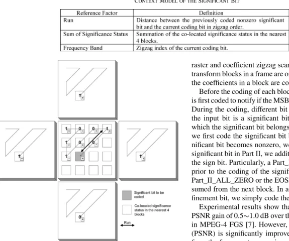
For efficiently coding significant bits, we jointly consider multiple factors as context model. We observe that 1) the nonzero coefficients with similar magnitude typically appear and cluster in zigzag scanning path; 2) the co-located coefficients in the spatially adjacent transform blocks have similar magnitude; and 3) the correlation varies with the frequency band. During the bit-plane coding, the significance status approximately reveals the magnitude of a coefficient. Thus, through the significance status, we map our observations into meaningful context model in Table II. For better understanding, Fig. 2 depicts an example of our context model for the significant bit. According to Table II, we can tell that the “Run” index is 1, the “Sum of Significance Status” is 3, and the “Frequency Band” is 8.

3) Refinement Bit: The refinement bit represents less

pre-dictable information. Statistical analysis shows that the refine-ment bits in the lower bit-planes may make up 50% or more. Thus, the coding efficiency of refinement bits is critical to the rate-distortion performance at high bit rates. Instead of using a fixed context probability model for all the refinement bits [5], [8], we use an estimated Laplacian model to derive the coding probability for each refinement bit. There is no context model specifically designed for the refinement bit. In Section IV, we use an example to illustrate how to calculate the coding proba-bility for a refinement bit.

4) Sign Bit: The sign bit records the sign of a coefficient.

Statistical analysis reveals that the distribution of a transform coefficient is approximately symmetric with respect to zero, i.e., the sign bit averagely consumes one bit. Thus, we use a fixed probability model for the coding of sign bits.

5) End-of-Significant-Bit-Plane (EOSP): The EOSP symbol

notifies the end of significant bit coding in a bit-plane. The lo-cation of EOSP reveals the energy distribution in a transform block. Through the spatial correlation, we can predict the loca-tion of EOSP by taking the average of the zigzag indices from the EOSP symbols in the nearest four neighbors. Particularly, when the adjacent EOSP used for prediction is not reached yet, we use the zigzag index of the last nonzero significant bit as replace-ment. With the predicted location, we define the context model of EOSP symbol as the offset (range: ) between the pre-dicted EOSP location and the currently coded nonzero

signifi-TABLE II

CONTEXTMODEL OF THESIGNIFICANTBIT

Fig. 2. Example of the context model for the significant bit. The transform block is with 42 4 integer transform.

cant bit. In addition, we jointly consider the bit-plane index as another factor since the distribution of offset values varies for each bit-plane. From the MSB bit-plane to the LSB bit-plane of a block, the bit-plane index is increased by one from zero. To save memory, the bit-plane index greater than 4 is truncated.

6) Part_II_ALL_Zero: The “Part_II_All_Zero” symbol

noti-fies the decoder about the all zero case of Part II. Table I shows that such event is unevenly distributed. Moreover, the probability distribution varies for each bit-plane. Thus, we take the bit-plane index as the context model of Part_II_ALL_Zero symbol.

D. Context Dilution Problem

In our CABIC, the number of context probability models in-creases with the transform size. For example, the context model of significant bit takes the coefficient zigzag index as one of the reference factors. Larger transform size requires more context probability models that cause context dilution problem. Exper-imental results show that the context dilution problem leads to worse coding efficiency. To reduce the number of context prob-ability models, our CABIC adopts the 4 4 integer transform [14] for the coding of the enhancement layer.

E. Coding Flow Using Raster and Zigzag Scanning

With the context model for each type of bits, the enhance-ment-layer frame is coded from the MSB bit-plane to the LSB bit-plane. In each bit-plane, the coding is performed in a frame

raster and coefficient zigzag scanning manner. Specifically, the transform blocks in a frame are ordered with raster scanning and the coefficients in a block are coded in zigzag order.

Before the coding of each block, a MSB_REACHED symbol is first coded to notify if the MSB bit-plane of a block is reached. During the coding, different bit types are coded differently. If the input bit is a significant bit, we examine the partition to which the significant bit belongs. For a significant bit in Part I, we first code the significant bit by itself. When the coded sig-nificant bit becomes nonzero, we further code a sign bit. For a significant bit in Part II, we additionally code an EOSP bit after the sign bit. Particularly, a Part_II_ALL_Zero symbol is coded prior to the coding of the significant bits in Part II. When the Part_II_ALL_ZERO or the EOSP is true, the coding will be sumed from the next block. In addition, if the input bit is a re-finement bit, we simply code the rere-finement bit by itself.

Experimental results show that our CABIC scheme offers a PSNR gain of 0.5 1.0 dB over the VLC-based bit-plane coding in MPEG-4 FGS [7]. However, although the objective quality (PSNR) is significantly improved, the poor subjective quality from the frame raster scanning still remains.

III. STOCHASTICBITRESHUFFLING

To improve the subjective quality, we propose a content-aware SBR scheme. Instead of using the frame raster and coef-ficient zigzag scanning, we propose to reshuffle the coefcoef-ficient bits of each bit-plane in a stochastic rate-distortion sense.

The concept and criterion of bit reshuffling was first pro-posed in [6] for improving the rate-distortion performance of wavelet-based image codec. For the reshuffling, in [6] each co-efficient bit is first assigned with two factors that are the squared error reduction and the coding cost . With these param-eters, the coefficient bits are reshuffled such that the associated is in descending order. By the equal slope concept of rate-distortion optimization theory, such order leads to min-imum distortion at any bit rates. However, the actual and of each coefficient bit are generally not available at decoder. Thus, the estimated and are used to avoid the transmis-sion of coding order. With the same estimation scheme at both encoder and decoder, the coding order is implicitly known to both sides. Equation (1) shows the condition of optimal coding order in the stochastic rate-distortion sense, where denotes taking estimation, the subscripts of and represents the bit identification, and the one of specifies the coding order

Fig. 3. Probability distributions of the 42 4 integer transform coefficients. The legend ZZn denotes the zigzag index of a coefficient and the KLD stands for the Kullback–Leibler distance [2]. (a) Actual probability distributions. (b) Estimated probability models.

In this paper, we employ the same concept for the bit reshuf-fling at the enhancement layer. Particularly, our estimation in-corporates the context probability model to make the priority assignment content aware so that the subjective quality can be improved. Moreover, we follow the optimized coding order in (1) to provide similar or even better rate-distortion performance.

IV. PARAMETERESTIMATION

To estimate the and for a coefficient bit, we resort to their expected values. In this section, we show how we use a discrete Laplacian distribution and context probability models to estimate the rate-distortion function for a 4 4 integer trans-form coefficient.

A. Discrete Laplacian Distribution

For calculating the expectations of and , we need the probability distribution of each transform coefficient. Since the actual distribution is only available at encoder side, we adopt a model-based approach to minimize the overhead. Specifically, we model each 4 4 integer transform coefficient with a dis-crete Laplacian distribution, as defined in (2), where de-notes the th zigzag-ordered coefficient of block and stands for its outcome. Particularly, we assume the co-located coefficients are independently and identically distributed (i.i.d.). Thus, the Laplacian parameter only depends on the zigzag index

(2) To estimate the Laplacian parameter, we use maximum like-lihood principle. Given a set of observed data and a pre-sumed joint probability with an unknown parameter, the max-imum likelihood estimator for the unknown parameter is the one that maximizes the joint probability. For an enhancement-layer frame with 4 4 blocks, the joint probability for the th zigzag-ordered coefficients can be written as in (3). According

to the i.i.d. assumption, we can simplify the joint probability as multiplication terms. Further, by substituting (2) into (3), we can obtain a close form formula for the joint probability as follows:

(3) By definition, the maximum likelihood estimator of is the one that maximizes (3). To find the solution, we take the deriva-tive with respect to and solve for the root. We leave the detail derivation in Appendix A. Based on (3), (4) shows our max-imum likelihood estimator for the

(4) According to (4), to estimate the for a coefficient, we first calculate the mean of absolute values of the co-located coefficients, , and then substitute it into (4) to obtain the estimator. Specifically, the estimation is done at the encoder and the estimated parameters are transmitted to the decoder. For each enhancement-layer frame, we have 16 parameters for the luminance component and another 16 parameters for the chrominance part. Particularly, each parameter is quantized and coded with a 8-bit syntax at frame level. Thus, for each enhance-ment-layer frame, additional 256 bits are coded as overhead. As compared to the entire bit-stream, the overhead is just a minor portion.

Fig. 3 compares the estimated distributions with the actual ones. As shown, the actual distributions are close to Laplacian and the estimated models preserve the relative distributions of different coefficients. To show the accuracy of our estimation,

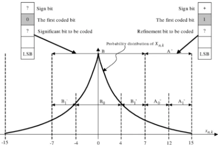
Fig. 4. Examples of1D estimation for the significant bit and refinement bit.

we calculate the Kullback–Leibler distance1_{(KLD) [2], which}

is a common measure for showing the difference between the actual distribution and its estimation. A KLD of value 0 means that the estimated distribution is identical to the actual one. As shown in Fig. 3(b), the KLD between our estimated distribu-tions and the actual ones approaches zero; that is, our estimated distributions are close to the actual ones.

B. Estimation of Delta Distortion

To estimate the for a coefficient bit, we use the reduction of expected squared error. Since the decoding of a coefficient bit is to reduce the uncertainty for a coefficient, we can calculate the reduction of expected squared error from the decrease of uncertainty interval.

Fig. 4, we depict the estimated distribution of a 4-bit coeffi-cient and give two examples for illustrating the decrease of un-certainty interval. Without loss of generality, the left-hand side shows an example of a significant bit, where the first bit is coded as zero. On the other hand, the right-hand side illustrates the case of refinement bit, where the first bit is nonzero.

From the coded bits, we can identify the uncertainty interval in which the actual value is located. For instance, in the ex-ample of significant bit, we know that the actual value is con-fined within the interval . Similarly, for the case of refinement bit, we learn that the actual value falls in the interval . Given the interval derived from the previously coded bits, the next bit for coding is to further decrease the uncertainty interval. For example, the significant bit to be coded is to determine that the actual value is in the subinterval or . Particularly, for a significant bit of nonzero, an additional sign bit is coded to further decide that the actual value is in the subinterval or . By the same token, the refinement bit to be coded is to determine that the actual value is in the subinterval or .

From the decrease of uncertainty interval, we can calculate the reduction of expected squared error. At decoder side, the ex-pected squared error in an interval is the variance within the in-terval. Thus, we can express our estimation as the reduction of variance. Equation (5) formulates our estimation for the

1_{KLD(P (x); P (x)) = P (x) log (P (x)=P (x)), where P (x) is the}

actual probability distribution andP (x) is its estimation.

case of significant bit in Fig. 4, where de-notes the conditional variance of given that is in the interval . Similarly, we have the variances for the subintervals , , and . Since we do not know in which subinterval the actual value is located, the variance of each subinterval is further weighted by its probability. To simplify the expression, we find that the variances of and are identical because Lapla-cian distribution is symmetric. So, we can merge the second and the third terms in (5) by factorization. Appendix B gives the de-tail derivations for the conditional probability and conditional variance in terms of interval range and

(5) In (5), the co-located significant bits within the same in-terval have the same estimated because the co-located coefficients have identical Laplacian model. The priorities of the co-located significant bits may not be distinguishable. To perform the reshuffling in a content-aware manner so that the regions containing more energy are with higher priority, in (5) the subinterval probabilities are replaced with the context probability models. Recall that the context model of signif-icant bit refers to the significance status of the adjacent and co-located coefficients. Using the context probability model for substitution makes the estimation become content aware and energy dependent.

For the substitution of subinterval probabilities in (5), we find that

actually denotes the probability of nonzero for the significant

bit to be coded and represents

its probability of zero. Hence, we use the associated context probability models to substitute for these two terms. Equation (6) shows the content-aware estimation for the example of significant bit in Fig. 4, where

denotes the context probability of nonzero for the significant bit of that locates in the interval . Correspondingly, the represents its probability of zero.

Following the same procedure, one can estimate the for the other bits. Equation (7) shows the estimated for the case of refinement bit in Fig. 4. Since the refinement bit does not have any context probability model, the conditional probabilities in (7) are derived from an estimated Laplacian model

(7)

C. Estimation of Delta Rate

To estimate the for a coefficient bit, we use the binary entropy2_{, which represents the minimum expected coding bit}

rate for an input bit. Equation (8) defines our estimation for the significant bit in Fig. 4. The first term represents the binary entropy of a significant bit using the context probability model as an argument while the second term denotes the cost from a sign bit. The sign bit is considered as partial cost of the signifi-cant bit because the decoder can only perform the reconstruction after the sign is received. Recall that each sign bit averagely con-sumes one bit. Also, the sign bit is only coded after a significant bit of nonzero. Thus, the cost of the sign bit is weighted by the context probability model of nonzero

(8) In addition, (9) illustrates our estimation for the example of refinement bit. To calculate the binary entropy, we use the conditional probability of a subinterval as an argument. For

in-stance, we use as an argument in

(9). In particular, as mentioned in Section II, such an estimated probability is not only for the calculation of binary entropy, but also for the CABIC coding. By the same methodology, one can estimate the for the other bits

(9) V. DYNAMIC PRIORITY MANAGEMENT FOR

STOCHASTICBITRESHUFFLING

Given the estimated rate-distortion performance for each co-efficient bit, in this section, we further show how these data are used for the SBR. Firstly, we illustrate our constraints for the reshuffling. Then, we present the dynamic priority management for the SBR. Lastly, we use an example to illustrate the idea.

A. Constraints of Reshuffling Order

In our algorithm, we pose two constraints on the reshuffling order to maintain low complexity and high coding efficiency.

2_{H (P (1))= 0P (1)2log (P (1))0(10P(1))2log (10P(1)), where}

P(1) is the nonzero probability of the coding bit.

These constraints make our implementation suboptimal in the stochastic rate-distortion sense. Specifically, they are as follows. • For an enhancement-layer frame, the coding is conducted

sequentially from the MSB bit-plane to the LSB bit-plane.

This constraint is to keep low complexity. Ideally, the reshuffling should allow the coefficient bits at different bit-planes be coded in an interleaved manner. However, in practical implementation, such flexibility requires a huge amount of coding states and branch instructions. Thus, in this paper, we perform the SBR in a bit-plane by bit-plane manner.

• For each bit-plane of a transform block, the coding of the

significant bits in Part II always follows zigzag order.

This constraint is to maintain high coding efficiency. Re-call that the coding of the significant bits in Part II will stop as the actual EOSP is reached. Since the location of EOSP is not known in advance, we follow zigzag order for the coding of the significant bits in Part II to prevent the re-dundant bits after EOSP from coding.

B. Dynamic Priority Management

To maintain the coding priority, we implement two dynamic coding lists for the reshuffling of significant bits and refinement bits. Each type of bits in the associated list allocates a register to record its bit location and estimate rate-distortion data. For syn-chronization, both encoder and decoder follow the same proce-dure to manage the lists. Sequentially, the management scheme includes the following five steps.

1) Coding List Initialization: Before the coding of each bit-plane, we estimate the rate-distortion data for the following bits and put them in the associated coding lists: 1) all the significant bits in Part I; 2) all the first zigzag-ordered sig-nificant bits in Part II; and 3) all the refinement bits in the current bit-plane.

2) Coding List Reshuffling: After the initialization, we per-form the reshuffling, according to the estimated rate-dis-tortion data, to identify the highest priority bit in the lists, i.e., the one with maximum . In addition, the reshuffling is performed after the coding of each bit. 3) Binary Arithmetic Coding: Once the highest priority bit

is identified, we follow the CABIC scheme in Section II for coding.

4) Rate-Distortion Data Update: After the coding of a nonzero significant bit, we update parts of the rate-dis-tortion data in the list of significant bit. Such update is to guarantee that our priority assignment is based on the latest context probability model. Moreover, through the update, we can fully utilize the coded information to enhance the effectiveness of content-aware bit reshuffling. Specifically, whenever a significant bit of nonzero is coded, we search in the coding list and update the registers for the following significant bits.

• Category 1: The significant bits that have the same con-text index as the current coded one.

• Category 2: The co-located significant bits in the adja-cent blocks.

• Category 3: The significant bits in Part I that locate after the current coded one (in zigzag order).

Fig. 5. Example of dynamic bit reshuffling in a bit-plane.

Updating the significant bits of Category 1 is necessary since the context probability model is refined after the coding. By the same token, updating the significant bits of Categories 2 and 3 is essential because the associated context indices have changed. Recall that the context model of significant bit refers to the significance status of the adjacent and co-located coefficients. Since all the coefficients are initialized with insignificant status, the context indices for those significant bits in Categories 2 and 3 are changed as the coded coefficient becomes significant. Therefore, we must update their rate-distortion data. Particularly, the rate-distortion data of the refinement bit is not required for update because it is derived from the estimated Laplacian model, which is fixed throughout the reshuffling process.

5) Significant Bit Inclusion: From our reshuffling con-straints, the coding of the significant bits in Part II always follows zigzag order. Thus, whenever a significant bit in Part II is coded, we estimate the rate-distortion data for the next zigzag-ordered significant bit and put it in the list. To complete the coding of a bit-plane, Steps 2 5 are repeated. When the coding of a bit-plane is done, we repeat Steps 1 5 until all the bit-planes are coded.

For better understanding, in Fig. 5, we use an example to il-lustrate the reshuffling process, where the binary number in each rectangle represents the content of a coefficient bit and its sub-script denotes the bit identification. For simplicity, we only illus-trate the reshuffling of significant bits. One can follow the same procedure to reshuffle the refinement bits. Practically, after the reshuffling of each list, we compare the highest priority bit in each list to identify the one for coding.

In the example of Fig. 5, we simplify the priority calculation as the summation of “(3-Run)” and the “Sum of Significance Status” that is defined in Table II. With our definition, the coef-ficient bits that have a shorter run and more significant coeffi-cients in the adjacent blocks will be assigned with higher coding priority. Specifically, to calculate the priority for each bit, the significant bits to be coded are first initialized with insignifi-cant status and the refinement bits are considered as signifiinsignifi-cant.

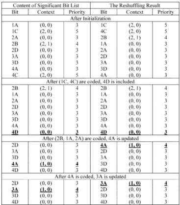
TABLE III

LIST OF THESIGNIFICANTBITDURING THEBITRESHUFFLING

Thus, for the bit 1C, its “Sum of Significance Status” is 2 and its “Run” index is 0. According to our definition, the bit 1C has a priority value of 5. By the same procedure, the priorities for the other significant bits can be obtained.

In Table III3_{, we present the content of significant bit list}

for the example in Fig. 5. On the right-hand side of Table III, we show the reshuffling result based on the coding priority. As shown, for the initialization, the coding list first includes the sig-nificant bits in Part I and the first zigzag-ordered sigsig-nificant bits in Part II. Then, according to the priority, the reshuffling is per-formed. Table III shows that 1C has the highest priority after the reshuffling. Hence, we start the coding form the 1C. After 1C is coded, we skip Step 4 because the adjacent and co-lo-cated coefficients have become significant. There are no signifi-cant bits to be updated. In addition, Step 5 is also skipped since 1C is the EOSP of a block. As a result, after the coding of 1C, we directly perform the coding for 4C. Particularly, after 4C is coded, we skip Step 4 for the same reason as the 1C. However, we include 4D in the list according to Step 5. The following 2B, 1A, and 2A are coded similarly. But, after 2A is coded and becomes nonzero, we update the rate-distortion data of 4A ac-cording to Step 4. As illustrated in Table III, the 4A becomes the one with the highest priority after the update and reshuf-fling. Therefore, we resume the coding from 4A. By continuing the procedure, one can finish the coding of significant bits and obtain the coding order as

. In particular, with the reshuf-fling, 2B is coded prior to 2A, which means that the significant bits in Part I could be coded in an order other than zigzag. We

3_{Context=(Summation of co-located significance status in the nearest four}

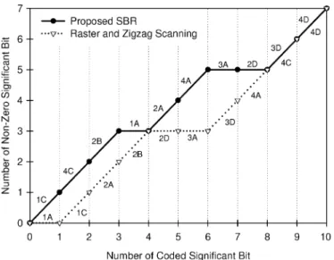
Fig. 6. Comparison of number of nonzero significant bits with different coding orders.

use such flexibility to allow optimization. As compared to the frame raster and coefficient zigzag scanning,

, Fig. 6 shows that our SBR has more significant bits of nonzero among the same number of coded significant bits. Generally, a signif-icant bit of nonzero contributes more to the error reduction at decoder.

VI. DYNAMICMEMORYORGANIZATION

The reshuffling and update process causes intensive com-putation. With straightforward implementation, the estimated rate-distortion data of all coefficient bits must be updated after the coding of a nonzero significant bit; then, the reshuffling is conducted using all coefficient bits as input. From the profiling of foreman CIF sequence on P4 2.0-GHz machine, it takes about 30 min for the bit-plane encoding4 _{of an enhancement-layer}

frame, which is unacceptable and unrealistic. Thus, in this sec-tion, we propose a dynamic memory organization to reduce the complexity of SBR.

A. Memory Management for the List of Significant Bit

For reducing the complexity of update and reshuffling, we observe that not all the registers are required for modification after the coding of a nonzero significant bit. Thus, we can mini-mize the computation by updating those outdated registers while keeping the others untouched.

To update the outdated registers, we first search them in the list. To quickly identify the registers of Category 1, we group the registers recording the same context index by a linked list. The right-hand side of Fig. 7 shows an example, where each circle denotes the associated register of a significant bit and each rectangle represents a context group. In each group, the registers with the same context index are grouped by a linked list. In addition, to identify the registers of Categories 2 and 3, we avoid exhaustive searching by confining our search within certain context groups. To determine which context groups for

4_{The bit-plane coding at the enhancement layer has balanced complexity in}

encoder and decoder.

search, we follow the definitions of Categories 2 and 3 to de-rive the bit locations for those outdated significant bits. From the bit locations, we further calculate their context indices be-fore the coding by reversing the significance status of the cur-rently coded bit. These context indices then determine the con-text groups for search. Within a group, we perform the search by comparing the bit location. Then, we update the outdated rate-distortion data using the latest context probability model.

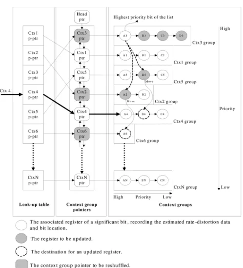
After the update, we perform the reshuffling in a hierarchical way. Specifically, we first identify the highest priority bit in each group. Then, we assign each group a context group pointer that points to the highest priority bit in a group. Lastly, we reshuffle the context group pointers to find out the highest priority bit in the list. Note that we do not directly reshuffle the highest priority bit of each group since we want to maintain the same context group structure. Particularly, the reshuffling in each group and the reordering of all the context group pointers are performed in the initialization step. During the actual coding, we only modify certain context groups and context group pointers so that the computation for reshuffling is minimized. Fig. 7 shows an ex-ample of our priority structure. For each group, the priority from left to right is in descending order. Similarly, for different groups, the priority of the highest priority bit from top to bottom is in descending order, i.e., we have

. In this example, A3 is not only the highest priority bit of Ctx3 group, but also has the highest priority in the list.

During the reshuffling and update, we must quickly access a context group for a given context index. To avoid exhaustive search in the linked list of context group pointers, we construct a look-up table that takes the context index as input and produces the associated context group pointer. The left-hand side of Fig. 7 depicts an example of the look-up table.

To show our dynamic memory organization, we use Fig. 7 as an example, where we assume that the registers in each group and the context group pointers have been reshuffled since the initialization. According to our priority structure, we start the coding from A3. Moreover, we assume the context indices of relevant registers B5 and A2 must be changed as A3 is recog-nized significant. To perform the reshuffling, after A3 is coded, we first update the rate-distortion data for the registers in the same group, i.e., B3, C3, and D3. Next, we update the rate-dis-tortion data of B5 and A2. Then we move B5 and A2 to the other context groups since their context indices have been changed. Specifically, the destination groups are determined by their con-text indices after A3 becomes significant. For example, in Fig. 7, the register B5 is updated and moved from the Ctx5 group to the B4 position of the Ctx4 group. Similarly, the register A2 is updated and moved from the Ctx2 group to the Ctx6 group. Par-ticularly, we put B5 at the location of B4 because the priority in

the Ctx4 group is .

After the update and movement for the relevant context groups (i.e., Ctx groups 3, 5, 2, 4, and 6), the highest priority bits of Ctx3, Ctx2, and Ctx6 groups have been changed. Thus, we must determine their new positions in the linked list of the context group pointers. To do so, we first remove the context group pointers (i.e., Context group pointers 3, 2, and 6) from the linked list. Then, we sequentially insert them back at proper positions by comparing the registers of the highest priority

Fig. 7. Dynamic memory organization for the list of the significant bit.

TABLE IV

AVERAGEEXECUTIONTIME FOR THEBIT-PLANEENCODING OF ANENHANCEMENT-LAYERFRAME ONP4 2.0-GHz MACHINE

TABLE V

ENCODERPARAMETERS FOR THEEXPERIMENTS

after the update. Particularly, the linked list of context group pointers is bidirectional. We can easily remove any context group pointer from the list. In this example, we only modify the

contents of the context groups 3, 5, 2, 4, and 6 while keeping the others untouched. The computation for update and reshuffling is minimized.

Fig. 8. Luminance PSNR comparison of baseline (VLC-based bit-plane coding in MPEG-4 FGS), baseline with frequency weighting, the proposed CABIC with frame raster and coefficient zigzag scanning, and the proposed CABIC with SBR.

B. Memory Management for the List of Refinement Bit

For the refinement bit, we only reshuffle the registers for iden-tifying the highest priority one. There is no need for update and relocation. Thus, we simply use a linked list to maintain the list of the refinement bit.

As compared to straightforward implementation, Table IV shows that a relative improvement ratio of more than 48 is achieved. Although the performance is still far way from real-time, more improvements are expected by further optimizing in both algorithmic and coding aspects.

VII. EXPERIMENTS

In this section, we assess the rate-distortion performance and subjective quality of our proposed scheme. For a fair compar-ison, all the schemes implemented adopt H.264 JM4 [14] as the base layer and RFGS [4] as the prediction scheme for the en-hancement layer. Specifically, we use the VLC-based bit-plane coding [7] as baseline. Moreover, we show the performance of baseline with frequency weighting. To compare the rate-distor-tion performance, our decoder truncates the bit-stream of the en-hancement layer at multiple bit rates and measures the PSNR of

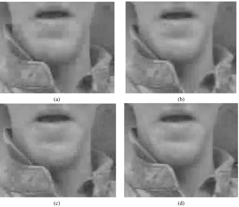
Fig. 9. Subjective quality comparison of the 94th frame in Foreman CIF sequence with bit rate at 255 kbits/s. (a) Baseline (VLC-based bit-plane coding in MPEG-4 FGS). (b) Baseline with frequency weighting. (c) Proposed CABIC with frame raster and coefficient zigzag scanning. (d) Proposed CABIC with SBR.

decoded video respectively. In addition, to compare the subjec-tive quality, we show the decoded frames of different approaches at the same bit rate. Table V lists our encoder parameters. For each sequence, different coding schemes use identical encoder parameters. In particular, to setup the frequency weighting ma-trix for the baseline, we follow the rule in [7] to have the coef-ficients of a lower frequency be coded with higher priority.

In Fig. 8, we compare the PSNR of different approaches at various bit rates. As shown, enabling the frequency weighting on the baseline causes a PSNR loss of 2 3 dB. Conversely, as compared to the baseline, our CABIC with frame raster and co-efficient zigzag scanning improves the PSNR by 0.5 1.0 dB at medium and high bit rates. Particularly, up to 2 dB gain can be observed in the News QCIF sequence. On the other hand, at the lower bit rates, the gain is less significant because the trun-cation of the enhancement layer causes drifting errors [4] and

the proposed CABIC takes time for the convergence of context probability models. In addition, our SBR can further offer up to 0.2 0.5 dB improvement.

While maintaining similar or even higher coding efficiency, our SBR offers better subjective quality. Fig. 9 shows the comparison of visual quality using Foreman CIF sequence. For better assessment, we have enlarged the regions where the subjective quality shows noticeable differences. As shown, the baseline and our CABIC with frame raster and coefficient zigzag scanning reveal obvious blocking artifact. On the other hand, the frequency weighting can provide smoother quality. But, the edge and texture parts are blurred because the co-efficients of higher frequency are always with lower coding priority. In contrast, our CABIC with content-aware SBR not only provides more uniform quality, but also keeps the details of edge and texture.

VIII. CONCLUSIONS

In this paper, we propose a CABIC with a SBR scheme to deliver higher coding efficiency and better subjective quality for FGS video coding. For higher coding efficiency, we construct context models based on both the energy distribution in a block and the spatial correlations in the adjacent blocks. Moreover, we exploit the context across bit-planes to save side information. Experimental results show that our CABIC provides a PSNR gain of 0.5 1.0 dB over the VLC-based bit-plane coding [7].

Further, for better subjective quality, our SBR combines con-text probability models and estimated Laplacian distributions to reorder coefficient bits in such a way that the estimated rate-distortion performance is in descending order. As compared to the approaches with frame raster and coefficient zigzag scan-ning, our SBR provides better visual quality and maintains sim-ilar or even higher coding efficiency.

This work proves that the bit-plane coding in MPEG-4 FGS [7] can be further improved in coding efficiency and subjec-tive quality by additional complexity. However, as compared to the nonscalable H.264 [14], there is still a performance gap of 2 4 dB with our testing conditions. To further reduce the gap, the proposed scheme can be improved with the stack FGS algo-rithms and hierarchical prediction schemes [3], [12] used in the current scalable video coding standard.

In addition to coding efficiency and subjective quality, an-other important issue that is not discussed in this paper is error resilience. Due to the data dependency from the context models and the nature of arithmetic coding, the proposed CABIC and bit reshuffling are less robust to transmission errors. For error resilience, one of the possible solutions is to partition the en-hancement-layer frames into multiple slices as the flexible mac-roblock ordering (FMO) in H.264 [14]. However, penalty on coding efficiency is expected. Thus, how to provide the op-timal tradeoff between coding efficiency and error resilience still leaves lots of spaces for future research activities.

APPENDIXA

This appendix shows the derivation of maximum likelihood estimator for the Laplacian parameter, . To maximize (3), the must be the root of (A1). For simplification, we have incorporated a logarithm function in (A1) to transform the exponential terms into additions/subtractions. Since logarithm function is monotonic, the root of (A1) is also the one that maximizes (3)

(A1)

After taking the derivative with respect to , (A1) can be rewritten as (A2)

(A2)

Since is a real number between 0 and 1, we exclude the root that does not meet such a constraint. Equation (A3) shows the remaining solution of that maximizes (3).

(A3) APPENDIXB

This Appendix shows the detail expressions for the condi-tional probability and variance. Without loss of generality, we use the example of refinement bit in Fig. 4 for illustration. Eq.

(B1) lists the definition of . Since the

segment in Fig. 4 is contained in the segment ,

in (B1) can be simplified as . By substituting (2) into (B1), we can further obtain the formula for

(B1)

In addition, (B2) lists the definition of

. As shown in (B2), the calculation of conditional variance involves the conditional expectation. To compute such an in-termediate result, (B3) defines the conditional th moment of

given

(B2)

(B3) By substituting (B3) and (2) into (B2), (B4) shows the formula for the

For the calculation of the other conditional probabilities and variances in (6)–(9), one simply needs to modify the ranges of summation in (B1) and (B4).

REFERENCES

[1] Y. Chen, R. Hayder, and M. van der Schaar, “Fine Granular Scal-able Video With Embedded DCT Coding of the Enhancement Layer,” DN/20030133499, U.S. patent application.

[2] T. M. Cover and J. A. Thomas, Elements of Information Theory. New York: Wiley, 1991.

[3] H. C. Huang and T. Chiang, “Stack robust fine granularity scalability,” in Proc. IEEE Int. Symp. Circuits and Systems, Vancouver, BC, Canada, 2004.

[4] H. C. Huang, C. N. Wang, and T. Chiang, “A robust fine granularity scalability using trellis based predictive leak,” IEEE Trans. Circuits Syst. Video Technol., vol. 12, no. 6, pp. 372–385, Jun. 2002. [5] N. K. Laurance and D. M. Monro, “Embedded DCT coding with

sig-nificance masking,” in Proc. IEEE Int. Conf. Acoustics, Speech, Signal Processing, Munich, Germany, 1997.

[6] J. Li and S. Lei, “An embedded still image coder with rate-distortion optimization,” IEEE Trans. Image Process., vol. 9, no. 7, pp. 297–307, Jul. 2003.

[7] W. Li, “Overview of fine granularity scalability in MPEG-4 standard,” IEEE Trans. Circuits Syst. Video Technol., vol. 11, no. 3, pp. 301–317, Mar. 2001.

[8] D. Nister and C. Christopoulos, “An embedded DCT-based still image coding algorithm,” in Proc. IEEE Int. Conf. Acoustics, Speech, and Signal Processing, Seattle, WA, 1998.

[9] W. H. Peng and Y. K. Chen, “Mode adaptive fine granularity scal-ability,” in Proc. IEEE Int. Conf. Image Processing, Thessaloniki, Greece, 2001.

[10] W. H. Peng, T. Chiang, and H. M. Huang, “Context based binary arith-metic coding for fine granularity scalability,” in Proc. IEEE Int. Symp. Signal Processing and its Applications, Paris, France, 2003. [11] W. H. Peng, C. N. Wang, T. Chiang, and H. M. Hang, “Context adaptive

binary arithmetic coding with stochastic bit reshuffling for advanced fine granularity scalability,” in Proc. IEEE Int. Symp. Circuits and Sys-tems, Vancouver, BC, Canada, 2004.

[12] J. Reichel, H. Schwarz, and M. Wien, Scalable Video Coding Working Draft 2 , ISO/IEC JTC1/SC29/WG11 and ITU-T SG16 Q.6, JVT-O201, 2005.

[13] J. M. Shaprio, “Embedded image coding using zerotrees of wavelet coefficients,” IEEE Trans. Signal Process., vol. 41, no. 12, pp. 3445–3462, Dec. 1993.

[14] T. Weigand, Draft ITU-T Recommendation and Final Draft In-ternational Standard of Joint Video Specification (ITU-T Rec. H.264—ISO/IEC 14496-10 AVC) , ISO/IEC JTC1/SC29/WG11 and ITU-T SG16 Q.6, JVT-G050, 2003.

[15] F. Wu, S. Li, X. Sun, B. Zeng, and Y. Q. Zhang, “Macroblock-based progressive fine granularity scalable video coding,” Int. J. Imaging Syst. Technol., vol. 13, no. 6, pp. 913–924, 2003.

Wen-Hsiao Peng was born in Hsinchu, Taiwan,

R.O.C., in 1975. He received the B.S. and M.S. degrees (with highest distinction) in electronics engineering in 1997 and 1999, respectively, from National Chiao-Tung University, Hsinchu, where he is currently pursuing the Ph.D. degree at the Institute of Electronics.

In 2000, he joined Intel Microprocessor Research Laboratory, Santa Clara, CA, where he developed the first real-time MPEG-4 FGS codec and demon-strated its application in a 3-D, peer-to-peer video conferencing. Since 2004, he has actively participated in ISO’s Moving Picture Expert Group (MPEG) digital video coding standardization process and contributed to the development of MPEG-4 Part 10 AVC Amd.1 scalable video coding (SVC) standard. His major research interests include scalable video coding, video codec optimization, and platform-based architecture design for video compression. He has published over 20+ technical papers in the field of video and signal processing.

Tihao Chiang (S’91–M’95–SM’99) was born in

Chia-Yi, Taiwan, R.O.C., in 1965. He received the B.S. degree in electrical engineering from the National Taiwan University, Taipei, in 1987, the M.S. degree in electrical engineering in 1991 and the Ph.D. degree in electrical engineering in 1995, both from Columbia University, New York.

In 1995, he joined the David Sarnoff Research Center, Princeton, NJ, as a Member of Technical Staff, and was later promoted to Technology Leader and Program Manager. While at Sarnoff, he led a team of researchers and developed an optimized MPEG-2 software encoder. In September 1999, he joined the faculty at National Chiao-Tung University, Hsinchu, Taiwan. Since 1992, he has actively participated in ISO’s Moving Picture Experts Group (MPEG) digital video coding standardization process with particular focus on the scalability/compatibility issue. He is currently the co-editor of Part 7 of the MPEG-4 Committee and has made more than 90 contributions to the MPEG Committee over the past ten years. His main re-search interests are compatible/scalable video compression, stereoscopic video coding, and motion estimation. He holds 13 U.S. patents and 30 European and worldwide patents and has published over 50 technical journal and conference papers in the field of video and signal processing.

Dr. Chiang was a co-recipient of the 2001 Best Paper Award from the IEEE TRANSACTIONS ONCIRCUITS ANDSYSTEMS FORVIDEOTECHNOLOGY. For his work in the encoder and MPEG-4 areas, he received two Sarnoff achievement awards and three Sarnoff team awards.

Hsueh-Ming Hang (S’79–M’80–SM’91–F’02) received the B.S. and M.S. degrees from National Chiao-Tung University (NCTU), Hsinchu, Taiwan, R.O.C., in 1978 and 1980, respectively, and the Ph.D. degree in electrical engineering from Rensselaer Polytechnic Institute, Troy, NY, in 1984.

From 1984 to 1991, he was with AT&T Bell Labo-ratories, Holmdel, NJ, and then joined the Electronics Engineering Department, NCTU, in December 1991. He has been actively involved in international video standards since 1984 and his current research inter-ests include multimedia compression, image/signal processing, and multimedia communication systems. He holds eight patents (R.O.C., U.S., and Japan) and has published over 130 technical papers related to image compression, signal processing, and video codec architecture.

Dr. Hang was an Associate Editor of the IEEE TRANSACTIONS ONIMAGE

PROCESSING (1992–1994) and the IEEE TRANSACTIONS ON CIRCUITS AND

SYSTEMS FORVIDEOTECHNOLOGY (1997–1999). He is co-editor and con-tributor of the Handbook of Visual Communications (published by Academic Press). He received the IEEE Third Millennium Medal and the IEEE ISCE Outstanding Service Award.

Chen-Yi Lee (M’01) received the B.S. degree from

National Chiao-Tung University (NCTU), Hsinchu, Taiwan, R.O.C., in 1982 and the M.S. and Ph.D. degrees from Katholieke University Leuven (KUL), Leuven, Belgium, in 1986 and 1990, respectively, all in electrical engineering.

From 1986 to 1990, he was with IMEC/VSDM, working in the area of architecture synthesis for dig-ital signal processing (DSP). In February 1991, he joined the faculty of the Electronics Engineering De-partment, NCTU, where he is currently a Professor and Department Chair. His research interests mainly include VLSI algorithms and architectures for high-throughput DSP applications. He is also active in var-ious aspects of high-speed networking, system-on-chip design technology, very low-power designs, and multimedia signal processing. He served as the Director of the Chip Implementation Center (CIC), an organization for IC design pro-motion in Taiwan. He is now the Microelectronics Program Coordinator of the Engineering Division under the National Science Council of Taiwan.

Dr. Lee was the former IEEE Circuits and Systems Society Taipei Chapter Chair.