基於遺傳演算法之具有多模具限制的並行機台排程方法

全文

(1)國立高雄大學資訊工程所碩士論文. 基於遺傳演算法之具有多模具限制的並行機台排程方法 Parallel Machines Scheduling with Multiple Mold Constraints Based on Genetic Algorithms. 研究生：漆慶福撰指導教授：洪宗貝博士共同指導教授：李詠騏博士. 中華民國 103 年 7 月.

(2) 基於遺傳演算法之具有多模具限制的並行機台排程方法. 指導教授：洪宗貝博士國立高雄大學資訊工程所. 共同指導教授：李詠騏博士正修科技大學資訊管理系. 學生：漆慶福國立高雄大學資訊工程所. 摘要目前要求排程問題之最優解已普遍被認定是 NP-hard 的問題，因此最近許多學者使用遺傳演算法尋找排程近似最優解，其中許多人已經在效率和質量上找到可以接受的結果。在這項研究中，我們將討論分配在多個並行機器的工作與模具限制的調度問題。每個作業須限制一種工作模具在一部機器上執行，每部機器限制可使用的工作模具，每付模具的數量有限制。此外，每部機器第一份工作開始或機器因改變工作而更換模具時，必須考慮模具安裝時間。因此本文使用遺傳演算法處理上述機器排程問題。其中，使用基因染色體表示機器與模具的排程架構，進而生成一個群體。使用調整運算子，調整機 i.

(3) 器與模具的衝突，產生可用的排程及提高適應值。染色體交配使用雙點交叉重現新一代染色體。此外，使用反向突變和對換突變 2 種突變操作，防止基因演化陷入局部最優解。程式最後滿足一定世代演化以獲得最好的完工時間排程結果。從實驗結果，驗證了本文提供的演算法之有效性。. 關鍵字：排程，遺傳演算法，最大完工時間，並行機器，模具限制。. ii.

(4) Parallel Machines Scheduling with Multiple Mold Constraints Based on Genetic Algorithms Advisor: Dr. Tzung-pei Hong Institute of Computer Science and Information Engineering National University of Kaohsiung. Co-advisor: Dr. Yeong-chyi Lee Department of Information Management Cheng Shiu University. Student: Ching-fu Chi Institute of Computer Science and Information Engineering National University of Kaohsiung. ABSTRACT Finding optimal solutions of scheduling problems has generally been NP-hard. Recently, GA-based algorithms have been introduced to find nearly optimal solutions, and many of them have found acceptable results in both efficiency and quality. In this study, we discuss the scheduling problem of assigning jobs on multiple parallel machines with mold constraints. The mold constraint specifies that each job needs to be processed with specific molds on a machine and there is an arbitrary amount for each type of molds. Besides, different machines can mount iii.

(5) different molds. Setup time is also considered when a first job in a machine starts or when a machine changes molds. A GA-based scheduling algorithm is thus proposed for dealing with the. above. scheduling. problem.. In. the. proposed. scheduling. approach,. a. chromosome-generating procedure is designed to generate a population. The adjustment operators are then adopted for improving the fitness values and keeping them from conflict. A two-point crossover operator is adopted to reproduce the new generation of chromosomes. Moreover, two mutation operators, the reverse mutation and the swapping mutation, are used to prevent the solutions from trapping into the local optimum. The scheduling result with the best makespan is then outputted from the population when the terminal condition is met. Finally, experimental results are given to verify the effectiveness of the proposed algorithm.. Keywords: Scheduling, Genetic Algorithm, Makespan, Parallel Machines, Mold Constraints.. iv.

(6) Contents 摘要................................................................................................................................. i ABSTRACT ................................................................................................................. iii Contents ......................................................................................................................... v List of Figures ..............................................................................................................vii List of Tables ................................................................................................................. ix CHAPTER 1. Introduction ........................................................................................ 1. CHAPTER 2. Review of Related Works .................................................................. 5. 2.1. GA-based Scheduling Algorithms .............................................................. 5. 2.2. Process of GA ............................................................................................. 7. 2.3. Operators of GAs ........................................................................................ 8. CHAPTER 3. Problem Definitions ......................................................................... 10. 3.1. Problem Statement .................................................................................... 10. 3.2. Notation ..................................................................................................... 13. 3.3. Some Properties in Scheduling ................................................................. 13. 3.4. Scheduling with Mold Constraints ............................................................ 20. CHAPTER 4. The Proposed Algorithm .................................................................. 24. 4.1. Chromosome Presentation ........................................................................ 25. 4.2. Initialization .............................................................................................. 27. 4.3. Contradiction Avoidance ........................................................................... 28. 4.3.1 The contradictions with mold constraints ............................................ 28 4.3.2 The adjustment operator for avoiding contradictions .......................... 31 4.3.3 An example of dealing with the contradictions .................................... 33 4.4. Crossover Operator ................................................................................... 35. 4.5. Mutation Operator ..................................................................................... 37 v.

(7) 4.6. Adjustment Operators for Improving the Makespan ................................ 39. 4.6.1 Adjustment of job order ....................................................................... 41 4.6.2 Molds replacement ............................................................................... 42 4.6.3 Swapping machines .............................................................................. 43 4.7. The Proposed Scheduling Algorithm ........................................................ 46. 4.8. An Example............................................................................................... 48. CHAPTER 5. Experimental Results ....................................................................... 54. CHAPTER 6. Conclusions and Future Work .......................................................... 63. References .................................................................................................................... 64. vi.

(8) List of Figures Figure 3.1 A scheduling result for Example 3.1........................................................... 12 Figure 3.2 The scheduling result of Example 3.2 ........................................................ 16 Figure 3.3 Jobs swapping result in Example 3.3 ......................................................... 19 Figure 3.4 Jobs swapping result in Example 3.4 ......................................................... 20 Figure 3.5 Scheduling results with different mold selections in Example 3.5 ............ 22 Figure 4.1 The encoding schema ................................................................................. 25 Figure 4.2 The representation of the chromosome in Example 4.1 ............................. 26 Figure 4.3 The scheduling result in Example 4.1 ........................................................ 26 Figure 4.4 The scheduling result violating the mold constraints ................................. 30 Figure 4.5 Two parent chromosomes of Example 4.3 ................................................. 36 Figure 4.6 The offspring chromosomes generated by crossover operator ................... 37 Figure 4.7 A new chromosome generated by the reverse mutation ............................. 38 Figure 4.8 A new chromosome generated by the swapping mutation ......................... 39 Figure 4.9 The scheduling result for Example 4.4 ....................................................... 41 Figure 4.10 The adjustment of the job order in Example 4.5. ..................................... 42 Figure 4.11 The adjustment of the mold order in Example 4.6. .................................. 43 Figure 4.12 Scheduling result before adjustment in Example 4.7. .............................. 45 Figure 4.13 The adjusted scheduling result in Example 4.7. ....................................... 46 Figure 4.14 The schedule presented by chromosome C1 ............................................. 51 Figure 5.1 The schedule dataset generator ................................................................... 56 Figure 5.2 The screen shot of the scheduling program after the running the proposed algorithm .......................................................................................................... 57 Figure 5.3 The average makespan of the schedules by the two GA-based scheduling vii.

(9) algorithms for different numbers of jobs ......................................................... 58 Figure 5.4 The makespan of the schedules by the two GA-based scheduling algorithms for different numbers of machines ................................................................... 59 Figure 5.5 The makespan of the schedules by the two GA-based scheduling algorithms for different numbers of molds ........................................................................ 60 Figure 5.6 Comparisons along different ratios of the mold set-up time and the average job processing time .......................................................................................... 62. viii.

(10) List of Tables Table 3.1 The ten jobs in Example 3.1 ......................................................................... 11 Table 3.2 The amounts of the molds ............................................................................ 11 Table 3.3 The adoptable molds for each machine ........................................................ 12 Table 3.4 The processing time of each job in Example 3.2 ......................................... 15 Table 3.5 Five jobs and the used molds in Example 3.5 .............................................. 22 Table 4.1 Jobs and their adoptable molds in Example 4.2 ........................................... 29 Table 4.2 The molds for each machine in Example 4.2 ............................................... 30 Table 4.3 The number of molds in Example 4.3 .......................................................... 30 Table 4.3 Five jobs and the used molds in Example 4.4 .............................................. 40 Table 4.4 The amount of each mold ............................................................................. 40 Table 4.5 The adoptable molds for each machine ........................................................ 41 Table 4.6 Jobs, processing time and the adoptable molds in Example 4.7 .................. 44 Table 4.7 The property of the eight jobs ...................................................................... 49 Table 4.8 The amount of each mold ............................................................................. 49 Table 4.9 The adoptable molds for each machine ........................................................ 49 Table 4.10 The six initial chromosomes in the example .............................................. 50 Table 4.11 The improved chromosomes by the designed adjustment operators .......... 50 Table 4.12 The fitness values of all the chromosomes in the population .................... 51 Table 4.13 The generated offspring chromosomes ...................................................... 53 Table 5.1 The environment of the given experiments .................................................. 54 Table 5.2 The parameters for the proposed GA-based scheduling algorithm .............. 55 Table 5.3 The parameter settings of data set ................................................................ 61. ix.

(11) CHAPTER 1 Introduction Scheduling issues are encountered anytime and everywhere in real life. The common goal of these kinds of problems is to achieve the goal of attaining maximum efficiency by sharing resources. Examples include scheduling in the agro-food industry [19], sports competition scheduling [17], nurse’s scheduling in hospitals [21], production scheduling in wafer fabrication [7]. In this study, we focus on the scheduling problems of the processing machines in a factory. In a rapidly growing economic environment, industries are facing competitive issues about low-cost, better quality, shortened delivery times, and safety production concerns. It is therefore necessary to develop highly efficient strategies for optimizing the production schedules for their production lines and to facilitate the company's sustainable development [10]. However, the computation complexity for finding optimal solutions of scheduling problems is usually an NP-complete issue. Baker and McMahon pointed that the heuristic procedures were good ways to solve scheduling problems in the real-world applications [2]. In this study, we thus attempt to use genetic algorithms to solve some scheduling problems.. 1.

(12) Genetic algorithm (GA), inspired from the process of natural selection, is a well-known artificial intelligence approach for searching for nearly optimal solutions in a heuristic way. Selection, reproduction, crossover, mutation and other operators are adopted by GAs to find the most suitable individuals in a population. In biological terms, the Ponginaes (ape’s ancestors) took 14 million years to evolve into Homo sapiens [35]. A good evolution thus usually needs a long time, and therefore the genetic process cannot easily find satisfactory solutions in a short term especially when chromosome structure is complex. Therefore, genetic engineering was proposed to find a good human genetic structure [34][36]. Adopting the eugenics [38] to improve human genes can not only effectively avoid the congenital genetic-disorders and giving birth to defective children, but can also be used for genetically modified food (GMF) [37] to increase the food amount. This means that genetic engineering can effectively find a satisfactory solution over a short period of time. Therefore, in this study, the concept of genetic engineering is adopted in solving the scheduling problem for improving the quality of chromosomes for getting satisfactory solutions. In [18], Jou et al. discussed the identical-machine scheduling problems with mold constraints. Chien et al. [9] further proposed the post-adjusted operator to solve the scheduling problems with multiple machines and mold constraints. In their approach, the machines are assumed identical. 2.

(13) In this thesis, the scheduling problem to be dealt with is to assign a set of jobs to a set of parallel machines with different processing properties. Each job processed on a machine requires one of the given molds, and can only be processed one at a time on a machine. The processing time of each job is predefined and assumed to be the same on each machine. The molds need to be mounted on the machines before jobs start. Each mold has an arbitrary number of identical ones. Moreover, the setup time is required when the first job on a machine starts or when a job assigned on a machine needs mold change. The setup time is assumed to be a constant for simplicity, but can be easily extended to different values. The scheduling problem discussed here is non-preemptive. We then propose a GA-based scheduling algorithm to deal with the job. assigning. problem. mentioned. above.. In. the. proposed. algorithm,. a. machine-independent encoding schema is introduced and three adjustment operators are designed for improving the qualities of the possible schedules in the evolution process. The remainder of this thesis is organized as follows. Chapter 2 shows some related GA-based algorithms in solving scheduling problems. Chapter 3 explains the details of the scheduling problem to be solved. The proposed GA-based scheduling algorithm is introduced in Chapter 4. In Chapter 5, experimental results are given to. 3.

(14) verify the effectiveness and show the performance of the proposed algorithm. Finally, conclusions and future works are given in Chapter 6.. 4.

(15) CHAPTER 2 Review of Related Works 2.1 GA-based Scheduling Algorithms In the past, the scheduling issues for identical machines were studied by many researchers. This well-known problem was first introduced by Graham in 1966 [13]. In Smith’s [24] and Cramer & Nichael’s [11] studies, the solutions for solving the scheduling problems on a production line by using Genetic Algorithms (GAs) were proposed. Scheduling problems with penalties of earliness and tardiness were then considered by Sivrikaya-Serifoglu and Ulusoy [12]. Aryanezhad et al. proposed an approach by taking advantage of both LP-metric and genetic algorithms to solve the bi-criteria scheduling problem [1]. Zaidi et al. [32] proposed the GLS (Genetic Local Search) algorithm to minimize the total completion time on a single machine with release dates and precedence constraints. Chen et al. [6] considered a single machine scheduling problem by developing dominance properties according to the sequence swapping of two neighborhood jobs, and the simple genetic algorithm is adopted as the global searching procedure. For the flow-shop scheduling problem, Wang et al. [29] proposed the cEDA (compact estimation of distribution algorithm) to solve the hybrid flow-shop 5.

(16) scheduling problems. Wang et al. [28] first used the Niche Genetic Algorithm (NGA) to solve a flow-shop scheduling problem with family sequence-dependent setup time. A common due window was also considered for minimizing the sum of total earliness and tardiness of all jobs and for avoiding premature convergence of GAs. Li et al. [20] then proposed a heuristic algorithm based on GAs to minimize the total weighted completion time. For scheduling on multiple machines, Zhao et al. [33] discussed the crossover probability and the mutation probability to overcome the shortage of the rare ripe and heterogeneous search. Chang et al. [5] proposed a Two-phase subpopulation genetic algorithm (TPSPGA) to find a Pareto-optimal solution for a good average performance. Song et al. [25] proposed an efficient heuristic algorithm based on GAs for solving the parallel-machine scheduling problems that optimized operational efficiency and minimized urgent task completion time, equipment failures and other random events interference in large-scale jobs. Chen et al. [8] proposed a hybrid-coded genetic algorithm to find a near-optimal solution in the solar cell industry. Bozejko [3] proposed an algorithm based on the Tabu search method that excluded the construction process of blocks for critical paths. To increase the ability of a local search for GAs, the process of GAs is usually modified or combined with other algorithms. Tsujimura et al. [27] proposed two kinds 6.

(17) of processing methods for symbiotic genetic algorithm, the co-evolution process and the sub-evolution process, to find optimal solutions. Harrath et al. [15] proposed a two-phase GA-based method to solve the job-shop scheduling problem by considering preventive maintenance of machines, machine breakdown, and tool replacement. Song et al. [26] proposed the combination of genetic algorithms and ant colony algorithms to effectively improve the local search capabilities and to solve the job-shop scheduling problems. Gu et al. [14] proposed a stochastic expected-value model based on the stochastic programming theory by using Quantum Genetic Scheduling Algorithm (QGSA) to solve the stochastic earliness and tardiness parallel machine scheduling. Sanches et al. [23] proposed a modeling strategy based on adaptive GA (AGA) for dealing with the scheduling of manufacturing systems which simultaneously used machines and automated guided vehicles. The single machine scheduling problem - virus evolution genetic algorithm (SMSP-VEGA) was proposed to obtain the optimal scheduling sequences for tasks [16].. 2.2 Process of GA The reason why genetic algorithms have been adopted by most researchers is their ability of finding nearly optimized solutions in the field of combinatorial optimization. Especially, GAs are usually efficient and easy to implement. GAs 7.

(18) present possible solutions of a problem by encoding chromosomes, which are processed by the evolution operators including selection, reproduction, crossover and mutation. The final answer from GAs must be decoded from chromosomes. Therefore, chromosomes can be treated as a type of data structure of GAs. Therefore, a well-defined encoding schema to form chromosomes will affect the efficiency of memory and execution time. DITCGA, BITCGA and AITCGA are three kinds of chromosome encoding methods proposed by Wu and Li [31] for job-shop scheduling. Among them, the AITCGA code can react quickly to meet the scheduled performance. Chang et al. [4] proposed the Artificial Chromosome with Genetic Algorithm (ACGA) to minimize the total deviation. Chen et al. then proposed a bi-variants probabilistic model and added on the ACGA to solve single machine scheduling problems with sequence-dependent set-up time.. 2.3 Operators of GAs Ribeiro et al. [22] proposed five kinds of crossover operators including One Point Crossover (OX), Similar Job Order Crossover (SJOX), Uniform Order-based Crossover (UOBX), Partially Mapped Crossover (PMX) and Relative Job Order Crossover (RRX), to solve the single machine scheduling problem. Wang et al. [30] 8.

(19) used fuzzy assessment for job processing time and proposed a new Hybrid Crossover (HX) operator that was a combination of the four typical crossover operators: PMX, OX, Circle Crossover (CX) and Uniform Crossover (UN), to solve the single machine earliness and tardiness problem.. 9.

(20) CHAPTER 3 Problem Definitions 3.1 Problem Statement In this study, the scheduling problem to be dealt with is to assign a set of n jobs to a set of m parallel machines, each of which can be mounted with a specific set of molds, respectively. Each job requires one of the given molds to be processed on a machine. The processing time of each job is predefined, and is assumed to be the same on each of the machines. The molds have their limitation for being mounted on the given machines. There are an arbitrary number of identical ones for each mold. The setup time is required when the first job on a machine starts or when a job assigned on a machine needs mold change. Here, the setup time is assumed to be a constant for simplicity, but it is easily extended to handle different setup times. Besides, the scheduling problem considered here is non-preemptive. One job can be processed by one machine at a time. A simple example is given below to illustrate the scheduling problem to be solved.. Example 3.1. Assume a scheduling requirement includes ten jobs which are assigned. 10.

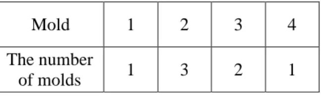
(21) on three machines to process while using four molds. Table 3.1 shows the profiles of the ten jobs to be scheduled. The processing time and the used mold candidates for each job are given in the rows. For instance, Job 1 takes six units of time and requires a machine mounted with Mold 2 or 4. Job 2 can only be processed by a machine with Mold 1 and needs seven units of processing time.. Table 3.1 The ten jobs in Example 3.1 Job. 1. 2. 3. 4. 5. 6. 7. 8. 9. 10. Processing Time. 6. 7. 4. 5. 8. 6. 6. 4. 5. 8. Molds. 2, 3. 1. 2, 4. 2. 4. 3. 1, 3, 4 1, 2, 3 3, 4 2, 3, 4. The numbers of molds can be different. In this example, the amounts of the molds are shown in Table 3.2.. Table 3.2 The amounts of the molds Mold. 1. 2. 3. 4. Amount. 1. 2. 2. 1. Machines are unrelated here, and thus each of them can be mounted with a specified set of molds. Table 3.3 depicts the set of molds which can be adopted for 11.

(22) machines. For instance, Machine A can use either Mold 1 or Mold 3.. Table 3.3 The adoptable molds for each machine Machine. A. B. C. Adoptable molds. 1, 3. 2, 3, 4. 1, 2. The elapsed time from the start to the finish of all the jobs in a schedule is known as makespan. When the setup time is given as 5, a scheduling result for Example 3.1 is shown in Figure 3.1, and the makespan of the schedule is 33.. Figure 3.1 A scheduling result for Example 3.1. 12.

(23) 3.2 Notation The notation used in this paper is listed as follows. J: a set of n jobs to be processed; M: a set of m machines to assign jobs for processing; H: a set of h mold types with arbitrary amounts; H(i): a subset of molds is suitable for job i, where H(i)  H; M(l): a subset of molds is adoptable to machine l, where M(l)  M; tj: the processing time of job j; hk: the amount of mold k; s: the setup time; J(i): the subset of jobs assigned to machine i, where i  M and J(i)  J; Li: the complete time of jobs executed on machine i.. 3.3 Some Properties in Scheduling In parallel machine scheduling problems with or without constraints, a set J of n jobs is to be processed on a set M of m machines. Assume a machine can process at most one job at a time and a job can only be assigned to a machine. That is, if i  j, then J(i)  J(j) = , where i, j  M. Besides, J(1)  J(2)  ...  J(m) = J, where J is the set. 13.

(24) of all jobs. The processing time for a job j  J is tj  . The final complete time of all the jobs on the machines is called the makespan. Let Li be the complete time of jobs loaded on machine i. Thus,. 𝐿𝑖 = ∑𝑗∈𝐽(𝑖) 𝑡𝑗 , where i  M.. The makespan is the maximum total processing time on any machine. Therefore, the makespan of a scheduling task is [39]:. 𝐿 = max𝑖 𝐿𝑖 , where i  M.. The goal of the makespan scheduling problem is to find the solution J* with minimum makespan L*. Therefore, 𝐿* = min(max𝑖∈𝑀 𝐿𝑖 ), where M is the set of given machines. There are several good properties for scheduling problems with the makespan criterion. The first one is the property of makespan lower bound in a feasible schedule [39], which is shown below.. Property 1. Let M be the set of given machines, m be the number of machines, and Li be the complete time of jobs loaded on machine I. Then, for any feasible schedule (including the optimal schedule), the lower bound of the makespan L in the schedule can be found as: 14.

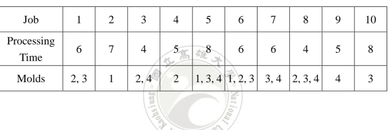
(25) 𝐿≥. ∑𝑖∈𝑀 𝐿𝑖 . 𝑚. The rationale of the above property can be shown below.. Proof. Let m be the number of machines. The complete time Li of each machine i will satisfy the following condition:. Li  max(L1, L2, …, Lm), 1  i  m.. The total complete time of all machines is thus: 𝑚. ∑ 𝐿𝑖 ≤ 𝑚 ∙ max(𝐿1 , 𝐿2 , ⋯ , 𝐿𝑚 ). 𝑖=1. Rewrite the above equation and we can get ∑𝑖∈𝑀 𝐿𝑖 ≤ max(𝐿1 , 𝐿2 , ⋯ , 𝐿𝑚 ) = max𝑖∈𝑀 𝐿𝑖 = 𝐿. 𝑚 Therefore, there is a lower bound,. ∑𝑖∈𝑀 𝐿𝑖 𝑚. , for the makespan L of a feasible. schedule.. Example 3.2. Assume that seven jobs (job 1 to job 7) are assigned to three machines (machine A, B, C). The processing time of each job is shown in Table 3.4. Table 3.4 The processing time of each job in Example 3.2 15.

(26) Job. 1. 2. 3. 4. 5. 6. 7. Processing Time. 5. 7. 4. 3. 9. 3. 5. Assume there are no additional constraints on the example. A scheduling result is shown as Figure 3.2. Since the complete time of each machine are: LA = t1 + t5 = 14, LB = t3 + t2 = 11, and LC = t4 + t6 + t7 = 11. Therefore, the makespan can be found as L = max(14, 10, 12) = 14. The makespan of the scheduling result cannot be smaller than the lower bound (14+10+12)/3, which is 12.. Figure 3.2 The scheduling result of Example 3.2. Below, we will describe the second property for improving a schedule for a better makespan.. Property 2. Assume machine k processes a set J(k) of jobs, and it takes the 16.

(27) longest complete time among all the machines, i.e. Lk = max𝑖∈𝐽(𝑘) 𝐿𝑖 = L. Assume that a job p  J(k) is processed on machine k with processing time tp, and another job q  J(j) is processed on another machine j with processing time tq. When 0 < tp – tq < Lk – Lj exists and no constraints are violated, a new smaller makespan L’ < L will be found after jobs p and q are exchanged between machines k and j.. Proof. It is known that machine k takes the longest complete time among all the machines. Thus, Lk = max𝑖∈𝐽(𝐾) 𝐿𝑖 = L. Since machine k processes job p  J(k) with processing time tp, its complete time can be rewritten as:. 𝐿𝑘 = ∑ 𝑡𝑖 = ( ∑ 𝑡𝑖 − 𝑡𝑝 ) + 𝑡𝑝 . 𝑖∈𝐽(𝑘). 𝑖∈𝐽(𝑘). Similarly, machine j processes job q  J(j) with processing time tq and its complete time can be rewritten as:. 𝐿𝑗 = ∑ 𝑡𝑖 = ( ∑ 𝑡𝑖 − 𝑡𝑞 ) + 𝑡𝑞 . 𝑖∈𝐽(𝑗). 𝑖∈𝐽(𝑗). After jobs p and q are swapped between machines k and j, if no constraints are violated, the new complete times, Lk’ and L j’, of machine k and machine j will become:. 𝐿𝑘 ′ = ( ∑ 𝑡𝑖 − 𝑡𝑝 ) + 𝑡𝑞 , 𝑖∈𝐽(𝑘). 17.

(28) 𝐿𝑗 ′ = ( ∑ 𝑡𝑖 − 𝑡𝑞 ) + 𝑡𝑝 . 𝑖∈𝐽(𝑗). To prove the new makespan L’ has been improved, we have to show L’ < L after the two jobs are swapped between machines. We thus first prove both Lk’ < L and L j’ < L as follows. Since Lk = max𝑖∈𝐽(𝐾) 𝐿𝑖 = L, then Lk’ – L = Lk’– Lk = ((∑𝑖∈𝐽(𝑘) 𝑡𝑖 − 𝑡𝑝 ) + 𝑡𝑞 ) − ((∑𝑖∈𝐽(𝑘) 𝑡𝑖 − 𝑡𝑝 ) + 𝑡𝑝 ) = tq – tp < 0, while 0 <tp – tq exists. Since Lk’ – Lk < 0, thus Lk’ < Lk = L is proved. Besides, when tp – tq < Lk – Lj, Lj’ – Lj = ((∑𝑖∈𝐽(𝑗) 𝑡𝑖 − 𝑡𝑞 ) + 𝑡𝑝 ) − ((∑𝑖∈𝐽(𝑗) 𝑡𝑖 − 𝑡𝑞 ) + 𝑡𝑞 ) = tp – tq < Lk – Lj = L – Lj. Therefore, Lj’ – Lj < L – Lj, and thus Lj’ < L is proved.. Furthermore, the complete times of all the other machines except machines p and q are certainly less than L since they are not changed. A new makespan L’, which is the maximum of the complete time, is thus less than L according to the above proof. The above property can thus be used to effectively decrease the value of makespan.. Example 3.3. Following Example 3.2, assume there is no constraint violated when job 1 on machine A and job 3 on machine B are swapped. The swapping result is shown 18.

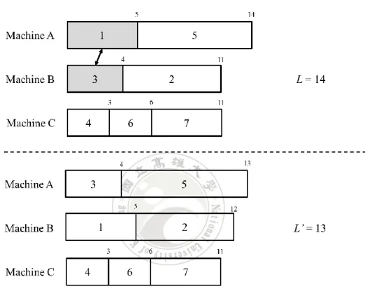
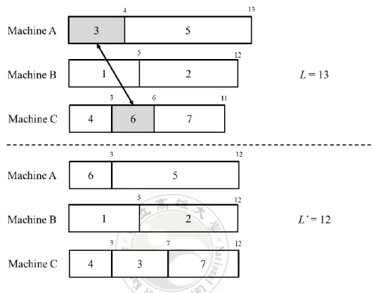
(29) in Figure 3.3. According to Property 2, the swapping will be beneficial to the makespan improvement, because LA – LB = 14 – 10 > t1 – t3 = 5 – 4. The new makespan L’ of the scheduling result is improved from 14 to 13.. Figure 3.3 Jobs swapping result in Example 3.3. Job exchanges will stop when the condition of 0 < tp – tq < Lk – Lj in Property 2 or some constraints are not matched. Example 3.4 is given to illustrate the situation of no job being swapped. Example 3.4. Continuing from above example, the makespan is updated again when jobs 3 and 4 are swapped between machines A and C, as shown in Figure 3.4. 19.

(30) After the swap, the makespan improves from 13 to 12. Since the condition of 0 < tp – tq < Lk – Lj in Lemma 2 does not exist, No more job swapping is done will be done.. Figure 3.4 Jobs swapping result in Example 3.4. 3.4 Scheduling with Mold Constraints In real applications, machines need to be mounted with some molds to be able to process jobs. This thesis thus considers the scheduling problems with mold constraints. The mold setup time is considered in two situations: (1) a machine loads its first job with a start mold; (2) molds change when jobs with different mold requirement are consecutively executed.. Therefore, the makespan of a schedule will increase when the. 20.

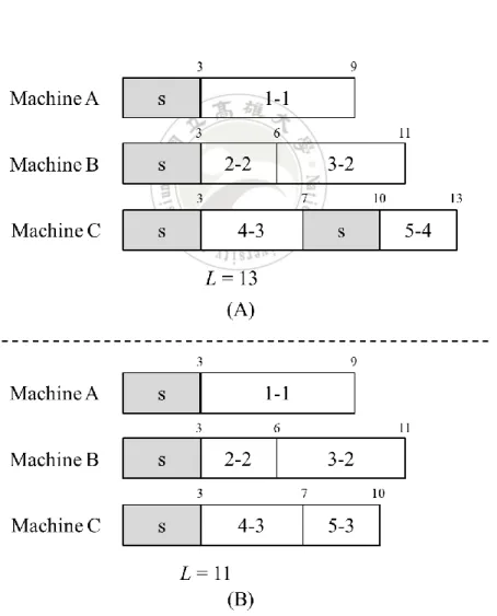
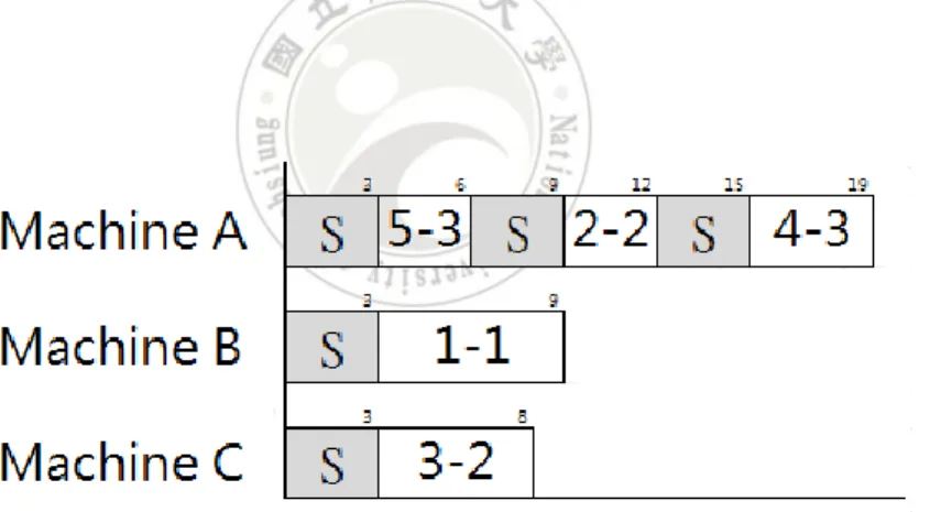
(31) molds installed on machines are changed often. For simplicity, the setup time is assumed to be a constant in this thesis. But arbitrary setup times for different modes can also be easily handled. Below, an example is given to illustrate the mold constraints.. Example 3.5. Five jobs are to be assigned on three machines, and the molds used by the jobs are shown in Table 3.5. Besides, assume that the molds can be installed on each machine. Job 3 can use molds 1 or 2 for processing, and job 5 can use molds 3 or 4. Different mold selection strategies for two scheduling results are presented in Figure 3.5, where s stands for setup time and a job is denoted by a job-mold pair which means that a specific mold is used by a job. For instance, job 1 assigned on machine A using mold 1 is denoted as 1-1 following a setup time in Figure 3.5(a). Assume that the setup time is given as 3 time units in this example. Each machine needs a setup time for installing the mold used by the first job. Since job 5 using mold 4 on machine C is different from job 4 using mold 3, a setup time for mold change is required in Figure 3.5(a). Therefore, the makespan of the scheduling result in Figure 3.5(a) is L = LC = 13. On the other hand, the makespan is L = LB = 11 when job 5 uses mold 3. There is no additional setup time needed for arranging job 5 to machine C in Figure 3.5(b). Therefore, to reduce the makespan, the setup time required on machines 21.

(32) needs to take as little as possible. That means, the frequency for mold change needs to be as small as possible.. Table 3.5 Five jobs and the used molds in Example 3.5 Job. 1. 2. 3. 4. 5. Processing Time. 6. 3. 5. 4. 3. Mold. 1. 2. 1, 2. 3. 3, 4. Figure 3.5 Scheduling results with different mold selections in Example 3.5. 22.

(33) As mentioned above, to reduce the makespan of the scheduling task, the cost of setup time on a machine should be as little as possible. Therefore, the mold selection for a job is important. Since the setup time is considered in this study, the lower bound of the makespan L in a feasible schedule is modified as:. 𝐿≥. ∑𝑖∈𝑀 𝐿𝑖 + 𝑠 ∗ 𝑚 ∑𝑖∈𝑀 𝐿𝑖 = + 𝑠. 𝑚 𝑚. The reason is that at least one setup time is required for installing the mold for the first job on each machine.. 23.

(34) CHAPTER 4 The Proposed Algorithm To deal with the scheduling problem as defined in Chapter 3. A GA-based algorithm is introduced in this chapter to find the optimal makespan on parallel machines while considering mold constraint. The mold constraint in this study is that each job can be processed by one of a set of specified molds on a machine and each type of mold has a given number of quantities. Besides, molds can only be installed on the specified machines, and the setup time is needed when the first job starts on a machine, or a job assigned on a machine when the installed mold is not matched with it. The setup time here is assumed the same for simplicity. The proposed GA-based scheduling algorithm is described in this section to solve the scheduling problem where a set of non-preemptive jobs and a set of machines with a set of molds are given to find the minimum for the completion time of each machine. The processing time of each job is assigned respectively, and it is the same while processing on each of the machines. The mold constraints and setup time mentioned above are also given. Therefore, the goal of the algorithm is to find the minimum makespan defined in Chapter 3.. 24.

(35) 4.1 Chromosome Presentation To present a possible solution in our GA-based algorithm, the encoded schema adopted in this study is shown in Figure 4.1. A possible solution is encoded as a chromosome with n gens, n is the number of jobs for scheduling, and each gene includes a triple of a job ji, a machine ki, and a mold mi, where i =1 to n. A gene of a chromosome stands for job ji which uses the mold mi being processed on a machine ki, where ji  J. Since a set of adoptable molds for each job are given as the mold constraints, the mold in each gene must be one of the adoptable molds for job ji, that is mi  H(i). Besides, jobs are assigned to machines according to the load of machines, and the machine with the lowest load is assigned jobs first. An example is given below for demonstrating the adopted encoding schema.. Figure 4.1 The encoding schema. Example 4.1. Assume that there is a set of five jobs and a set of three machines, and four kinds of molds are given for scheduling. Also assume that the number of each kind of mold is one. The chromosome shown in Figure 4.2 presents job 3 uses mold 2 on 25.

(36) machine A, and job 5 uses mold 1 on machine B, and so on.. Figure 4.2 The representation of the chromosome in Example 4.1. As the scheduling assignment encoded by the chromosome, the processing order of the jobs is job 3, job 5, job 1, job 4 and job 2. The scheduling result is shown in Figure 4.3 for the above chromosome. The first three jobs, job 3, job 5 and job 1, are assigned to machine A, machine B and machine C respectively in alphabetical order, and setup time is needed on each machine. Since the load of machine B is lowest when it turns to job 4 to be assigned, job 4 is then assigned to machine B. job 2 is processed on machine C which has the lowest load in turn to job 2. An additional setup time is needed between job 1 and job 2 on machine C, since they use different molds.. Figure 4.3 The scheduling result in Example 4.1. 26.

(37) 4.2 Initialization The first set of feasible solutions is required for updating during the evolution processes of a GA-based algorithm. Therefore, a set of chromosomes are randomly generated according to the above encoding schema, and each chromosome is mapped to be a corresponding possible schedule. The set of the n given jobs are randomly assigned to n genes of a chromosome, and the mold of each gene is randomly picked from the adoptable molds of respective jobs. No genes are assigned to the same job. The initially generated p chromosomes are formed as the initial population, where p is the defined size of a population. The method of generating chromosomes for a population is introduced as follows.. The chromosome generating procedure INPUT: A set of n jobs with processing times and their adoptable molds, a set of m machines, a set of h molds with given amounts. OUTPUT: A set of p chromosomes, where p is the size of the population.. STEP 1: Set i = 1, where i is an index of the i-th chromosome with n genes being generated. STEP 2: Set q = 1, where q is an index of the q-th gene with the triple of job, machine, 27.

(38) and mold, jq-kq-mq, being generated. STEP 3: Randomly select a job r from the given set J of jobs, r  J, and let jq = r. STEP 4: Set t is the machine with the lowest loading, t  M. Let kq = t. If the lowest loading is kept by multiple machines, then t is set in alphabetical order. STEP 5: Randomly select a mold s from the given set of molds adoptable to job r, s  H(r), and let mq= s. STEP 6: If q = n, then go to next step; otherwise, set q = q + 1, and return to STEP 3. STEP 7: Check if the contradiction about mold constraint happens, then the adjustment operator introduced in Section 4.3 is executed. STEP 8: If i = p, then stop the generating processes and output the n generated chromosomes; otherwise, set i = i + 1, and return to STEP 3.. 4.3 Contradiction Avoidance 4.3.1 The contradictions with mold constraints To keep chromosomes away from violation of the given mold constraints when new chromosomes are generated at initialization, or at reproduction, by executing the genetic operators, some contradictions may be found when mold constraints are considered. Therefore, the chromosome tuning operators is adopted to adjust the chromosomes which violate the given mold constraints. Two kinds of contradictions 28.

(39) may happen on a chromosome, and they are (1) the mold assigned to a job in a chromosome cannot be installed on the machine that processes the job; (2) the number of a mold is not enough to install on the machines that process the jobs using the same mold. Example 4.2 is given below to demonstrate these two contradictions.. Example 4.1. Assume the mold constraints are given as Table 4.1, Table 4.2 and Table 4.3. The adoptable molds for respective jobs are given in Table 4.1. In Table 4.2, the molds installed on respective machines are shown. The number of each mold can then be found in Table 4.3. Also assume that a chromosome, 1A4-3B2-2C1-4A1-5C1, is generated from the chromosome generating procedure in Section 4.3. And this chromosome represents the scheduling result which is shown in Figure 4.4.. Table 4.1 Jobs and their adoptable molds in Example 4.2 Job. 1. 2. 3. 4. 5. Time. 4. 4. 8. 10. 3. Molds. 3, 4. 1, 2. 2. 1. 1, 2, 4. 29.

(40) Table 4.2 The molds for each machine in Example 4.2 Machine. A. B. C. Molds. 1, 3. 2, 3. 1, 4. Table 4.3 The number of molds in Example 4.3 Mold. 1. 2. 3. 4. The number of molds. 1. 3. 2. 1. There are two contradictions being observed from in Figure 4.4. One is the first gene 1A4 of the chromosome, job 1 using mold 4 on machine A, violates the given mold constraint, since mold 4 used by job1 cannot be installed on machine A. The other is both gene 4A1 and gene 5C1 need mold 1 at the same time but there is only one mold 1 according to Table 4.3.. Figure 4.4 The scheduling result violating the mold constraints. 30.

(41) 4.3.2 The adjustment operator for avoiding contradictions The contradictions that illustrated in Section 4.4.1 could happen, when a chromosome is generated or it reproduces from the crossover operator and the mutation operator. To deal with the contradictions, an adjustment operator is proposed to avoid a chromosome violating the given mold constraints. The adjustment operator scans the genes of a chromosome one by one to check if they satisfy the given mold constraints. A gene is made of a triple, <j, k, m>, which means that job j is processed on machine k with mold m. Each gene is checked if job j with mold m is able to be processed on machine k. There are two situations for job j with mold m can be processed on machine k. The first is the used mold m cannot be installed on machine k, since mold m is not an adoptable mold of machine k. The second, the amount of the mold is not enough for installing on machines at the same time. In the proposed adjustment operator, the first situation is handled by replacing another suitable mold for the gene. After the first situation of contradictions is handled, if the contradictions are still found in the chromosome, the second situation is then dealt with. Another available machine that is suitable for job j is selected. If there are multiple choices of suitable machines, then find the lowest loading one.. 31.

(42) The adjustment operator for avoiding contradiction Input: A generated chromosome, C; the given mold constraints. Output: A chromosome without violating the mold constraints. STEP 1: Set C’= null, Tq1 = null, and Tq2 = null, where C’, Tq1 and Tq2 are temporal queues. STEP 2: Pop a gene from C, and set the gene as g. The triple of the gene g is denoted as a triple <j, k, m>. STEP 3: If the mold m of gene g is not adoptable to the assigned machine k, then push g to Tq1; otherwise, push g to C’. STEP 4: If C is empty, then go to STEP 5; otherwise, go to STEP 2. STEP 5: If Tq1 is empty, then go to STEP 7; otherwise, pop the a gene from Tq1 and set the gene as g. STEP 6: Select one of the suitable molds m’ of job j, where m’  H(j) ∩ M(k). The mold m is then substituted by m’. If there is no suitable mold for job j, then push g to Tq2; otherwise, push g to C’. Go to STEP 5. STEP 7: If Tq2 is empty, then go to STEP 9; otherwise, pop a gene from Tq2, and set the gene as g. STEP 8: Select one of the available machine k’ that is suitable for job j. If there are multiple choices of suitable machines, then find the lowest loading one. Set 32.

(43) k = k’, and push g to C’. Go to STEP 7. STEP 9: Set C = C’, and output the chromosome C.. 4.3.3 An example of dealing with the contradictions Example 4.2. Continue with Example 4.1, assume that the chromosome, 4A1-3B2-2C1-5C4-1B4, generated from the chromosome generating procedure in Section 4.3. In this example, we demonstrate the above chromosome is tuned by the proposed adjustment operator and output without violating the mold constraints.. STEP 1: Let C = 4A1-3B2-2C1-5C4-1B4, and set C’ = Tq1 = Tq2 = null. STEP 2: Pop a gene from C, and set as g, that is g = 4A1. STEP 3: Since gene g = 4A1 do not violate the mold constraints, it is then pushed to C’. STEP 4: Since C is not empty, go to STEP 2. STEP 2: Pop a gene from C, and set as g, that is g = 3B2. STEP 3: Gene g = 3B2 do not violate the mold constraints, it is then pushed to C’. Therefore, C’ = 4A1-3B2 STEP 4: Go to STEP 2, since C is not empty. STEP 2: Pop a gene from C, and set as g, that is g = 2C1. STEP 3: Gene g violates the mold constraints, since the number of mold 1 used by 33.

(44) job 2 of gene g is 1. Job 2 cannot be processed on machine C by using mold 1. Therefore, gene g is then pushed into Tq1. STEP 4: STEP 2 is executed while C is not empty. STEP 2 to STEP 4 carry out three times until C is empty. C’ = 4A1-3B2-5C4 and Tq1 = 2C1-1B4. STEP 5: Since Tq1 is not empty, then pop the first gene from Tq1 and set g = 2C1. STEP 6: Since the alternative mold that is suitable to job 2 is mold 2, and mold 2 cannot installed on machine C. Therefore, gene g is pushed into Tq2. STEP 5 is then processed. STPE 5: Set g as 1B4 popped from Tq1. STEP 6: The mold of gene g is replaced by mold 3, and machine B is suitable for it. Therefore, gene g is set as 1B3, and it is pushed into C’. C’ = 4A1-3B2-5C4-1C3, and Tq1 = null, Tq2 = 2C1. STEP 5: Tq1 is empty, and STEP 7 is then processed. STEP 7: Pop a gene from Tq2, and set g = 2C1. STEP 8: Change the machine of gene g to machine B, since the loading of machine B is the lowest and mold 1 is adopted by machine B. Therefore, gene g is set as 2B1. No contradiction happens on g = 2B1, then g is pushed into C’. C’ = 4A1-3B2-5C4-1C3-2B3. 34.

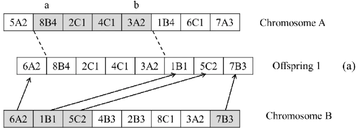
(45) STEP 7: Tq2 is empty, and then go to STEP 9. STEP 9: Set C = C’ = 4A1-3B2-5C4-1C3-2B3, and output the chromosome C.. 4.4 Crossover Operator Crossover is a main evolution operator of the genetic algorithm. Two chromosomes are randomly selected to exchange their genes to generate two new offspring chromosomes for further evolving. In this study, the two-point crossover is adopted to mate for the exchanging genes of two chromosomes. In the two-point cross operator, each of the offspring chromosomes inherits half of the genes from each of parents. One offspring inherits the half of chromosome, from a-th gene to b-th gen, and the remaining part of the offspring's chromosome comes from the other parent's genes, whose jobs are different from those between a and b. The point a is randomly assigned from 1 to (n/2 + 1), and point b is decided by a, that is b = a + (n/2 – 1), where n is the number of genes in a chromosome. After new offsprings are generated, the adjustment operators are performed to tune them from violating the mold constraints. Example 4.3 is given below for present the cross operator adopted in this study.. Example 4.3. Assume that chromosome A and chromosome B are both randomly selected from the population. These two chromosomes, shown in Figure 4.5, are chosen 35.

(46) to perform the two-crossover operator for generating new chromosomes as offsprings. When the cross point a is set at 2 and n = 8, then the cross point b is 2 + (8 / 2 – 1) = 5. In Figure 4.6(a), offspring 1 is generated by inheriting chromosome A's genes from 2-nd gene to 5-th gene, and the other genes come from chromosome B where the jobs are different from genes between gene 2 to gene 5 of chromosome A. In the same manner, the offspring mainly inherits from chromosome B and shown in Figure 4.6(b).. Figure 4.5 Two parent chromosomes of Example 4.3. 36.

(47) Figure 4.6 The offspring chromosomes generated by crossover operator. 4.5 Mutation Operator The mutation operator is seen as the secondary evolution operator in this study for helping the GA-based algorithm escape from the trap of searching the local optimum. Two mutation operators are adopted in this study: the reverse mutation operator and the swapping mutation operator. The details of these two mutation operators are described as follows.. 37.

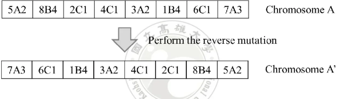
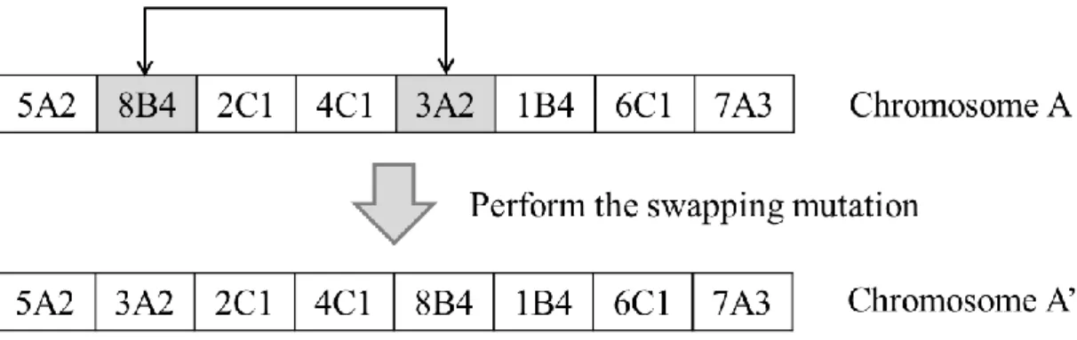
(48) a. The reverse mutation operator. When the reverse mutation operator is performed, the order of genes in a chromosome is reversed, and a new chromosome is then outputted. This kind of mutation is a mass change for reordering genes in a chromosome. It may be performed once on a new chromosome as it is newly generated. In Figure 4.7, chromosome A' is generated by performing the reverse mutation operator on chromosome A.. Figure 4.7 A new chromosome generated by the reverse mutation. b. The swapping mutation operator. The reverse mutation may be performed once on a new chromosome as it is newly generated. The swapping mutation is a minor change on a chromosome, and it swaps two genes of a chromosome with a certain probability. Figure 4.8 shows that chromosome A' is generated by performing the swapping mutation.. 38.

(49) Figure 4.8 A new chromosome generated by the swapping mutation. After mutation operators are performed, the adjustment operators are then used for tuning the chromosomes violating the mold constraints.. 4.6 Adjustment Operators for Improving the Makespan Once a scheduling solution is outputted by genetic operators, the following adjustment can improve the makespan. The adjustment operators are adopted in this study for improving the fitness of chromosomes. They are considered as the process of genetic modification when chromosomes are randomly generated. Three improvements we considered to adjust the structure of scheduling results for the improvement of the makespan, such as the adjustment of job order, replacement of molds, and swapping machines, are addressed as follows. A simple example is given below to illustrate the scheduling problem found in this study. 39.

(50) Example 4.4. Assume a scheduling requirement to be solved is that five jobs are assigned on three machines to process while using four molds. Table 4.3 shows the profiles of the ten jobs to be scheduled. The processing time and the using molds of each job are given in each column. For instance, to process Job 1 takes six units of time and requires a machine, which mounts with Mold 1 or Mold 3. Job 4 can only be processed by machines with Mold 3 and needs four units of processing time.. Table 4.3 Five jobs and the used molds in Example 4.4 Job. 1. 2. 3. 4. 5. Processing Time. 6. 3. 5. 4. 3. Mold. 1,3. 2,3. 1,2. 3. 2,3,4. The molds vary in amount in this study. The numbers of the molds are shown in Table 4.4.. Table 4.4 The amount of each mold Mold. 1. 2. 3. 4. Number of mold. 1. 2. 2. 1. Machines are unrelated here since each of them can be mounted with a specified set of molds. Table 4.5 depicts the sets of molds which are adopted by machines 40.

(51) respectively. For instance, Machine A can use Mold 2 and Mold 3.. Table 4.5 The adoptable molds for each machine Machine. A. B. C. Adoptable molds. 2, 3. 1, 3, 4. 1, 2. The time every machine takes for completing its assigned jobs of a scheduling task is known as the makespan. When the setup time is given as three, a scheduling result for Example 4.4 is shown in Figure 4.9, and the makespan of the job assignment is 19.. Figure 4.9 The scheduling result for Example 4.4. 4.6.1 Adjustment of job order The higher the frequency of mold replacement that happens on a machine, the more set-up time is needed for installing the molds to fit the jobs. If jobs using the same 41.

(52) mold on a machine are not continuously processed, it will cost multiple set-up times for switching molds. Therefore, the jobs using the same mold on a machine that are shifted together to be processed continuously can improve the scheduling results.. Example 4.5 Continuing with Example 4.4, both of Jobs 5 and 4 use Mold 3 but they are not processed continuously on Machine A, so that it needs the set-up time for installing Mold 3 twice. An improvement is taken that Job 4 is reordered from the last processing job following Job 5. The number of set-up times taken on Machine A is reduced from 3 to 2. The adjusted results are shown in Figure 4.10. Figure 4.10 The adjustment of the job order in Example 4.5.. 4.6.2 Molds replacement If a job with its adoptable molds is able to match with the mold used by its adjacent jobs on the same machine, replacing the mold is a feasible way to reduce set-up time for. 42.

(53) improving the scheduling results.. Example 4.6 Continuing with Example 4.5, replacing the mold of the Job 2, from Mold 2 to Mold 3, on the Machine A to match with Job 5’s mold can reduce the set-up time. The adjusted results are shown in Figure 4.11.. Figure 4.11 The adjustment of the mold order in Example 4.6.. 4.6.3 Swapping machines After scheduling results are outputted, the following adjustment can improve the makespan. The assignment of the machine J(k) with the largest complete time is considered being modified, and its complete time is denoted as Lk = L. According to Lemma 2, the makespan can be improved by swapping jobs between machines. Since the machines with complete time are lower than L* could be the factor that leads J(k) to have the largest complete time, so that one of them is picked to swap jobs with J(k) to. 43.

(54) improve the makespan if the condition of 0 < tp – tq < Lk – Lj in Lemma 2 exists. The adjustment processes are not stopped until the condition of 0 < tp – tq< Lk – Lj in Lemma 2 is not shown. Example 4.7 is given to show the adjustment strategy.. Example 4.7. A set of eight jobs are assigned to four machines to be processed, and five molds are given to be installed on machines for jobs. Table 4.6 shows the given jobs, their processing time and their adoptable molds. The setup time is given as five. A scheduling result is shown in Figure 4.12, and its makespan is 22. The dash line in Figure 4.12 presents the lowest bound of the makespan is 16.75.. Table 4.6 Jobs, processing time and the adoptable molds in Example 4.7 Job. 1. 2. 3. 4. 5. 6. 7. 8. Processing Time. 6. 3. 4. 9. 7. 4. 3. 9. Mold. 2, 4. 1, 5. 1, 3. 3. 4. 1, 2, 4 1, 3, 5 1, 2, 3. 44.

(55) Figure 4.12 Scheduling result before adjustment in Example 4.7.. The makespan has space to be improved, since the complete time of machine D, LD = L, can be reduced by swapping jobs with other machines while the condition of 0 < tp – tq < Lk – Lj in Lemma 2 exists. In Figure 4.13, the complete time of machine C is below L* and is the lowest one, so that job 4 on machine D and job 2 on machine C are chosen to swap, since 0 < t4 – t2 = 9 – 5 < LD – LC = 22 – 14. Job 4 can also use mold 1 used by job 6 while swapping to machine C to avoid additional setup time. After the job swapping, the makespan of the adjusted scheduling result is improved from 22 to 20, and it is shown in Figure 4.13.. 45.

(56) Figure 4.13 The adjusted scheduling result in Example 4.7.. 4.7 The Proposed Scheduling Algorithm In the proposed GA-based algorithm, the encoded schema and the chromosome generating procedure are derived to generate a population. A set of p chromosomes are randomly generated to form the initial population. The adjustment operator for improving the fitness of chromosomes is then adopted to be as a genetic modification to let chromosomes become a better makespan. A two-point crossover operator is adopted to reproduce the new generation of chromosomes. Moreover, two mutation operators, the reverse mutation and the swapping mutation, are used to prevent the solutions from trapping into local optimum. Another adjustment operator is then given for tuning the chromosomes that violate the given mold constraints and it is executed when new chromosomes are generated. The scheduling result with the best makespan is outputted from the population when the terminal condition is met. The processes of 46.

(57) the proposed GA-based algorithm are described as follows.. The GA-based scheduling algorithm with mold constraints INPUT: A set of n jobs with processing times and their adoptable molds, a set of m machines, a set of h molds with given amounts. OUTPUT: A feasible scheduling with the minimum makespan.. STEP 1: Execute the chromosome generating procedure in Section 4.3 for randomly generating a population of p chromosomes according to the encoding schema mentioned above. STEP 2: Check if there are contradictions existing in the chromosomes, adjust them with contradiction avoiding manner in Section 4.4 to keep from violating the mold constraints. STEP 3: Calculate the fitness of each chromosome as follows: 𝐿 = max𝑖𝑀 𝐿𝑖 , 𝐿𝑖 = ∑𝑗∈𝐽(𝑖) 𝑡𝑗 , i  M. Where M is the given set of the machine, Li is the complete time of machine i, and J(i) is the set of jobs processed on machine i with processing time tj. STEP 4: Perform the crossover operation on the population. 47.

(58) STEP 5: Perform the mutation operations on the population. STEP 6: Adjust the offspring generated from STEP 4 and STEP 5 by the designed adjustment operators, and adjust the offspring chromosomes if they violate the mold constraints. And then calculate the fitness of the offspring chromosomes. STEP 7: Check if there are contradictions existing in the chromosomes, adjust them with contradiction avoiding manner in Section 4.4 to keep from violating the mold constraints. STEP 8: Select the chromosomes with the best p fitness values for next generation. STEP 9: Repeat STEP 2 to 8until the termination criterion is satisfied. STEP 10: Output the schedule with the best makespan.. 4.8 An Example In this section, an example is given to illustrate the proposed scheduling algorithm. This is a simple example to show how the proposed algorithm can be used to find the scheduling with the minimum total tardiness under the mold constraint. Assume a scheduling requirement to be solved is that eight jobs are assigned on three machines to process while using four molds. Table 4.7 shows the profiles of the eight jobs to be scheduled. Table 4.8 shows the profiles of the four molds and table 4.9 shows the profiles of the three machines. Also assume that the set-up time is set as three. 48.

(59) Table 4.7 The property of the eight jobs Job. 1. 2. 3. 4. 5. 6. 7. 8. Processing Time. 5. 4. 6. 4. 7. 3. 6. 4. Mold. 3,4. 2,3,4. 1,4. 1,3. 1,2. 1,2,4. 2,3. 3. Table 4.8 The amount of each mold Mold. 1. 2. 3. 4. Number of molds. 1. 2. 2. 1. Table 4.9 The adoptable molds for each machine Machine. A. B. C. Adoptable molds. 1, 3. 1, 3, 4. 2,3,4. STEP 1: P individuals are randomly generated as the initial population according to the mentioned encoding scheme. Each individual thus represents a possible schedule. For example, assume p is set at six for simplicity. Assume the six initially generated individuals are shown in Table 4.10. STEP 2: Adjust the individuals by the designed adjustment operators for improving the structures of chromosomes. The result is shown in Table 4.11.. 49.

(60) Table 4.10 The six initial chromosomes in the example ID. Chromosomes. C1. 4A1-7B3-3C4-1A3-8B3-6C2-5B1-2A3. C2. 6A1-1B4-2C3-5A2-4C3-7B3-8C3-3C4. C3. 8A3-3B4-5C2-1A3-4B1-2C3-7A3-6B1. C4. 2A3-6B4-4C2-7B3-8A3-3C4-1A3-5B1. C5. 1A3-3B1-7C2-4A3-2B4-5C2-8A3-6A1. C6. 3A1-1B4-7C2-4B3-5A2-6C4-2B4-8C3. Table 4.11 The improved chromosomes by the designed adjustment operators ID. Adjusted Chromosomes. C1. 4A1-1B3-5C2-7A3-8B3-6C2-3B4-2A3. C2. 6A1-1B4-2C3-5A2-4C3-7B3-8C3-3C4. C3. 8A3-3B1-5C2-1A3-4B1-2C3-7A3-6B1. C4. 7A3-6B1-5C2-4B1-8A3-2B3-3C4-1A3. C5. 1A3-3B1-7C2-4A3-5B1-2C4-8A3-6B1. C6. 3A1-1B3-4C2-6C2-2B3-5A1-8C3-7B3. STEP 3: The fitness value of each chromosome is then calculated for the makespan 50.

(61) schedule. Take chromosome C1 as an example. The chromosome C1 is shown in Figure 4.14. The makespan of chromosome C1 is calculated as 21. The fitness values of all the chromosomes in the population are calculated with their results shown in Table 4.12.. Figure 4.14 The schedule presented by chromosome C1. Table 4.12 The fitness values of all the chromosomes in the population ID. L. C1. 21. C2. 24. C3. 18. C4. 19. C5. 19. C6. 18. STEP 4: Execute the adopted crossover operation on the population. Assume that the two chromosomes C1 and C2 are randomly chosen by the crossover operator to 51.

(62) generate offsprings. Assume that the crossover point a is randomly set at 1, point b is then as 1 + (8 / 2 – 1) = 4. The following two offspring chromosomes are generated as follows. The two mating chromosomes: C1: 4A1-1B3-5C2-7A3-8B3-6C2-3B4-2A3 C2: 6A1-1B4-2C3-5A2-4C3-7B3-8C3-3C4 The generated offspring chromosome: C1t’: 4A1-1B3-5C2-7A3-6A1-2C3-8C3-3C4 C2t’: 6A1-1B4-2C3-5A2-7C3-4B1-8C3-3B4. STEP 5: The reverse mutation is executed to generate possible offspring. Assume that the chromosome C5 is selected to execute the mutation operator. The following offspring chromosome is generated as follows. The selected chromosome: C5: 1A3-3B1-7C2-4A3-5B1-2C4-8A3-6B1 The chromosome generated from mutation: C5t’:6B1, 8A3, 2C4, 5B1, 4A3, 7C2, 3B1, 1A3. STEP 6: The offspring chromosomes are adjusted by the designed adjustment operator. 52.

(63) Assume that there are six newly generated offspring chromosomes reproduced from STEP 4 and STEP 5. The newly generated offspring chromosomes are shown in Table 4.13 and their fitness values are then evaluated.. Table 4.13 The generated offspring chromosomes ID. Newly generated chromosomes. L. C1t’. 4A3-2B4-5C2-1A3-6B4-3B4-7C3-8A3. 16. C2t’. 6A1-1B4-2A3-4A1-7C3-3B4-5A1-8C3. 17. C3t’. 8A3-3B1-5C2-7A3-1B3-6C2-4A3-2C2. 17. C4t’. 7A3-6B1-3C4-4B1-8A3-1C4-5B1-2A3. 17. C5t’. 8A3-5B1-6C2-2C3-4A3-7B2-3A1-1C3. 20. C6t’. 3A1-1B3-4C2-6C2-8B3-5A1-2C4-7B3. 18. STEP 7 to 9: The best chromosomes are selected as the next generation. The same procedure is then executed again until the termination criterion is satisfied. The best chromosome in the last generation is then outputted as the best scheduling result.. 53.

(64) CHAPTER 5 Experimental Results This chapter describes the experiments that were made to show the performance of the proposed GA-based algorithm for scheduling on unrelated parallel machines with the mold constraints. The following Table 5.1 shows the environment of the given experiments. Three parameters are considered to define the problem, number of jobs, number of machines, and number of molds. The experiments show the comparison of the proposed GA-based scheduling algorithms with and without the adjustment operators.. Table 5.1 The environment of the given experiments CPU. Intel(R) Core(TM) i5-3450 @3.10GHz 3.50GHz. RAM. 8.0 GB. OS. Microsoft windows 7 (64 bits). Program tools. Microsoft visual C#. Some related parameters for the proposed GA-based scheduling algorithm are shown in Table 5.2 as follows.. 54.

(65) Table 5.2 The parameters for the proposed GA-based scheduling algorithm Generation. 100. Population. 50. Mutation probability pm. 0.03. Setup time. 5. Since it is difficult to find a proper real-world dataset to exam the proposed scheduling algorithm in the following experiments, the synthetic datasets are thus considered as being adopted in the experiments. For this reason, a schedule dataset generator is then made to produce the synthetic datasets of the following experiments. A screen shot of the schedule dataset generator is shown in Figure 5.1. The properties of the synthetic datasets can be set such as the attributes of a project, the mutation modes, and the attributes of machines, jobs and molds.. 55.

(66) Figure 5.1 The schedule dataset generator. The experiments are implemented by Microsoft Visual C#, and the screen shot of the scheduling program executing our proposed scheduling algorithm and the simple GA without the adjustment operators is shown in Figure 5.2.. 56.

(67) Figure 5.2 The screen shot of the scheduling program after the running the proposed algorithm. In the first experiment, the job numbers are set at 20, 40, 60, 80 and 100, the machine number and the mold number are both set at 10. A set of molds between one to eight and the respective processing time are then randomly assigned to each job. Both methods are run 100 times and their makespan are kept. The averages of the makespan of the two GA-based scheduling algorithms for different numbers of jobs are shown in Figure 5.3.. 57.

(68) With Adjustement. Without Adjustment. 600. Makespan (Avg.). 500 400 300 200 100 0 20. 40. 60 Job numbers. 80. 100. Figure 5.3 The average makespan of the schedules by the two GA-based scheduling algorithms for different numbers of jobs. From Figure 5.3, it can be observed that the more number of jobs the higher the makespan to complete the assigned jobs. Moreover, it is easily seen that the proposed algorithm with the adjustment operator achieved a better result than without the adjustment operator. The proposed adjustment operators can thus obviously improve the scheduling results. In the second experiment, we devote time on the comparison with the makespan of the two GA-based scheduling algorithms for different numbers of machines, and the results are shown in Figure 5.4. In the experiments, the job number is set at 50, and the mold number is set at 10. The makespan of both methods are tested for different numbers of machines at 5, 10, 20 and 30. Each job is then randomly assigned a set of 58.

(69) one to eight molds and its processing time. Both methods are run 100 times and their makespan are kept. The averages of the makespan of the two GA-based scheduling algorithms for different numbers of machines are then shown in Figure 5.4.. With Adjustement. Without Adjustment. 600. Makespan (Avg.). 500 400 300. 200 100 0 5. 10 20 Machine Numbers. 30. Figure 5.4 The makespan of the schedules by the two GA-based scheduling algorithms for different numbers of machines. From Figure 5.4, it can also be easily seen that the proposed algorithm with the adjustment operator acquired a better result than that without the adjustment operator for any number of machines. Next, the makespan of the two GA-based scheduling algorithms for different numbers of molds are shown in Figure 5.5. In the experiments, the job number is set at. 59.

(70) 50, the machine number is set at 10and the mold numbers are set at 5, 10, 15 and 20. Each job is then randomly assigned a set of one to eight molds and its processing time.. With Adjustement. Without Adjustment. 350. Makespan (Avg.). 300 250 200 150 100 50 0 5. 10 15 Mold Numbers. 20. Figure 5.5 The makespan of the schedules by the two GA-based scheduling algorithms for different numbers of molds. From the comparison of results, it is easily observed that the proposed algorithm with the adjustment operator has the best makespan than that without the adjustment operator for the number of molds. From Figures 5.3, 5.4 and 5.5, we find the results with the adjustment operators are better than those without it. The adjustment operators do obviously improve the scheduling results on the machines with the mold constraints. In order to observe the influence of the mold set-up time on the makespan, an 60.

(71) experiment is made for comparing the GA-based scheduling algorithms with, and without, the adjustment operators along different ratios of the mold set-up time, and the average job processing time. The properties of the experiment are shown in Table 5.3.. Table 5.3 The parameter settings of data set Parameter. Value. The number of job. 25. The number of machine. 4. The number of mold. 5. A job average the process time. 31.2. A job average the number of using molds. 2.82. A machine average the suitable molds. 2.5. The average of the number of molds. 2.2. Figure 5.6 shows the results of the GA-based scheduling algorithms with and without the adjustment operators. The Y-axis represents the average makespan of the 100 times experiment, and X-axis represents the ratios of the mold setup time, and the average job processing time is set around 31.2.When the mold set-up time is set at 300, the ratio is thus as 1:10. It can be observed that the adjustment operators are more effective to reduce the makespan as the mold set-up time is much larger than the job processing time. 61.

(72) with Adjustment. without Adjustment. 1400 1200 1000 800 600 400 200 0 10:1. 5:1. 1:1. 1:5. 1:10. Figure 5.6 Comparisons along different ratios of the mold set-up time and the average job processing time. 62.

(73) CHAPTER 6 Conclusions and Future Work In this thesis, we have attempted to solve the scheduling problems that jobs are assigned to multiple unrelated machines with mold constraints. A GA-based scheduling algorithm is proposed for finding the minimum makespan of these problems. In the proposed algorithm, an encoding schema is introduced, and the adjustment operators are also given for improving fitness values of the chromosomes when they are generated. The proposed approach can be easily extended to solve the same problem, as well as the fitness function of the total complete time. Finally, the experimental results show that the adjustment operators are effective in avoiding the mold conflicts and are then able to receive better scheduling results. Thus, it can be shown that the scheduling results with the adjustment operators are much better than those without it. In the future, we will consider solving more related scheduling problems on tardiness issues by using different strategies. We will continue our research in other related fields.. 63.

(74) References [1] M. B. Aryanezhad, A. Jabbarzadeh, and A. Zareei, "Combination of Genetic Algorithm and LP-metric to Solve Single Machine Bi-Criteria Scheduling Problem", The IEEE International Conference on Industrial Engineering and Engineering Management, pp. 1915-1919, 2009. [2] J. R. Baker and G. H. McMahon, "Scheduling the General Job-Shop," Management Science, Vol. 31, No. 5, pp. 594-598, 1985. [3] W. Bożejko, M. Uchrŏnski, and M. Wodecki, "Multi-machine Scheduling Problem with Setup Times", Archives of Control Sciences, Vol. 22, No. 4, pp. 441-449, 2012. [4] P. C. Chang, S. S. Chen, Q. H. Ko, and C. Y. Fan, "A Genetic Algorithm with Injecting Artificial Chromosomes for Single Machine Scheduling Problems", IEEE Symposium on Computational Intelligence in Scheduling, pp. 1-6, 2007. [5] S. S. Chen, P. C. Chang, S. M. Hsiung, and C. Y. Fan, "A Genetic Algorithm with Dominance Properties for Single Machine Scheduling Problems", IEEE Symposium on Computational Intelligence in Scheduling, pp. 98-104, 2007. [6] P. C. Chang, S. H. Chen, and K. L. Lin, "Two-Phase Sub Population Genetic Algorithm for Parallel Machine-scheduling Problem," Expert Systems with Applications, Vol. 29, No. 3, pp. 705-712, 2005. [7] J. H. Chen, L. C. Fu, M. H. Lin, and A. C. Huang, "Petri-Net and GA-Based Approach 64.

(75) to Modeling, Scheduling, and Performance Evaluation for Wafer Fabrication", IEEE Transactions on Robotics and Automation, Vol. 17, No. 5, pp. 619-636, 2001. [8] C. Y. Cheng., T. L. Chen, L. C. Wang, and Y. Y. Chen, "A Genetic Algorithm for the Multi-Stage and Parallel-Machine Scheduling Problem with Job Splitting – A Case Study for the Solar Cell Industry", International Journal of Production Research, Vol. 51, No. 16, pp.4755-4777, 2013. [9] T. I. Chien, "Design of Efficient Heuristic Algorithms for Solving Scheduling Problems with Multiple Mold Constraints", Master Thesis, I-Shou University, 2010. [10] I. C. Choi and D. S. Choi. "A Local Search Algorithm for Job-shop Scheduling Problems with Alternative Operations and Sequence-Dependent Setups", Computers & Industrial Engineering, Vol. 42, No. 1, pp. 43–58, 2002 [11] N. L. Cramer, "A Representation for the Adaptive Generation of Simple Sequential Programs," The International Conference on Genetic Algorithms, pp. 183-187, 1985. [12] S. S. Funda and U. Gündüz, "Parallel Machine Scheduling with Earliness and Tardiness Penalties", Computers & Operations Research, Vol. 26, No. 8, pp. 773–787, 1999. [13]R. L. Graham, "Bounds for Certain Multiprocessing Anomalies," Bell System Technical Journal, Vol. 45, No. 9, pp. 1563–1581, 1966. [14] J. W. Gu, X. H. Gu, and B. Jiao, "Solving Stochastic Earliness and Tardiness Parallel 65.

(76) Machine Scheduling using Quantum Genetic Algorithm," The 7th World Congress on Intelligent Control and Automation, pp. 4154 - 4159, 2008. [15] Y. Harrath, J. Kaabi, M. B. Ali, and M. Sassi, "Multi-objective Genetic Algorithm-Based Method for Job Shop Scheduling Problem: Machines Under Preventive and Corrective Maintenance Activities", The 4th Conference on Data Mining and Optimization, pp. 13-17, 2012. [16] S. Hu, D. Chu, and X. Xu, "A Virus Evolution Genetic Algorithm for Scheduling Problem with Penalties of Independent Tasks on a Single Machine", The WRI Global Congress on Intelligent Systems, Vol.1, pp. 574-578, 2009. [17] G. D. Huang, P. Ling, and Q. Wang, "A Hybrid Meta-heuristic ACO-GA with an Application in Sports Competition Scheduling", The Eighth ACIS International Conference on Software Engineering, Artificial Intelligence, Networking, and Parallel/Distributed Computing, Vol. 3, pp. 611-616, 2007. [18] S. S. Jou, "Solving Scheduling Problems of Identical Machines with Mold Constraints Based on Genetic Algorithms", Master Thesis, National Kaohsiung Normal University, 2009. [19] A. Karray, M. Benrejeb, and P. Borne, "New Parallel Genetic Algorithms for the Single-Machine Scheduling Problems in Agro-food Industry", The 2011 International Conference on Communications, Computing and Control Applications, pp. 1-7, 2011. 66.