零和限制下探討證券商經營效率之研究

全文

(1)國立交通大學經營管理研究所博士論文 No.125 零和限制下探討證券商經營效率之研究 An Efficiency Study of the Securities Firms under the Zero-Sum Gains Constraint 研究生：方進義指導教授：胡均立. 教授. 中華民國九十八年一月.

(2) 國立交通大學經營管理研究所博士論文 No.125 零和限制下探討證券商經營效率之研究 An Efficiency Study of the Securities Firms under the Zero-Sum Gains Constraint. 研究生：方進義研究指導委員會：胡均立教授丁. 承教授. 唐瓔璋. 教授. 指導教授：胡均立. 教授. 中華民國九十八年一月 ii.

(3) 零和限制下探討證券商經營效率之研究 An Efficiency Study of the Securities Firms under the Zero-Sum Gains Constraint 研究生：方進義. Student：Chin-Yi Fang. 指導教授：胡均立. Advisor：Dr. Jin-Li Hu. 國立交通大學經營管理研究所博士論文 A Dissertation Submitted to Institute of Business and Management College of Management National Chiao Tung University in Partial Fulfillment of the Requirements for the Degree of Doctor of Philosophy in Business and Management January 2009. Taipei, Taiwan, Republic of China. 中華民國九十八年一月. iii.

(4) 零和限制下探討證券商經營效率之研究研究生：方進義. 指導教授：胡均立. 國立交通大學經營管理研究所博士班. 摘. 要. 台灣證券市場因政府鼓勵金融控股公司成立而競爭更趨激烈，金控公司提供了全方位之金融服務：包括銀行、證券與保險等業務。目前文獻中，研究金控母公司對於其證券子公司效率之影響的相關實證研究甚少，缺乏個別證券公司的資料造成了實證研究的困難，更遑論研究金控對於其證券子公司之管理效率的影響。目前傳統之資料包絡分析模式從事的研究，並未考慮在總和產出有限制情況下（如證券商之短期目標為爭奪市占率，但市占率之總和為 100%）作經營效率之評估，其所衡量的經營效率值有低估的現象。因此，本研究以 2001 年至 2005 年台灣綜合券商為觀察對象，所有變數經由 GDP 平減指數轉成以 2001 年為基期的實質變數，以去除物價變動的影響，以探討在零和限制下券商經營效率之研究，實證研究顯示：外資券商的所有權對經營效率呈現顯著正向影響，二階段最小平方法（The two-stage least squares procedure）確認了市占率與經營效率之聯立關係。接著再利用 Fried 等人於 1999 年發展的四階段資料包絡分析模式（Four-stage data envelopment analysis）評估台灣綜合券商之管理效率。實證研究顯示：在主管機關主導下所成立之金控公司對於其證券子公司之管理效率是有顯著之不良影響；顯示台灣在法令誘導成立下的金控公司，並非是有效率之綜合券商與銀行合組金控；成立年限愈久的券商相對其效率亦愈高；整體而言，成立金控後的確對券商市場造成威脅與改善整體的證券商經營效率。關鍵詞：四階段資料包絡分析法、縱橫面資料、證券商成立年限、證券子公司、零和限制之資料包絡分析法、二階段最小平方法、股權結構. iv.

(5) An Efficiency Study of the Securities Firms under the Zero-Sum Gains Constraint Student: Chin-Yi Fang. Advisor: Dr. Jin-Li Hu. Institute of Business and Management National Chiao Tung University ABSTRACT Taiwan’s government has been actively promoting financial holding companies (FHCs), which offer various services including banking, securities and insurances.. The issue of whether or. not the FHC system can effectively improve a securities firms’ managerial efficiency is still not empirically studied.. The lack of firm-level data has made research on securities firms (SFs) very. difficult and rare to see, not to mention the effects of FHC on their managerial efficiency. Current studies that use traditional data envelopment analysis (DEA) neglect the 100% market share restriction.. This study adopts zero-sum gains data envelopment analysis (ZSG-DEA) to. measure the efficiency scores of SFs and indicates that the traditional DEA model underestimates the efficiency scores of inefficient SFs.. This research analyses 266 integrated securities firms (ISFs) in. Taiwan from 2001 to 2005 and employs three inputs (fixed assets, financial capital, and general expenses) and a single output (market share). deflator with 2001 as the base year. efficiency scores.. All nominal variables are transformed by GDP. The foreign-affiliated ownership of SFs positively affects the. The two-stage least squares procedure (2SLS) confirms that the market share. and efficiency score simultaneously reinforce each other. The four-stage DEA proposed by Fried et al. (1999) is then further applied. subsidiaries under the law-induced FHCs are not the efficient ISFs in Taiwan. significantly negative effect on the managerial efficiency of an ISF. also significantly improves its efficiency score.. The securities An FHC has a. A higher duration of an ISF. Meanwhile, forming FHCs imposes a threat and. creates the incentives for efficiency increasing in the securities industry. Keywords: Four-stage data envelopment analysis (DEA); Panel data; Duration; Securities subsidiaries; Zero-sum gains data envelopment analysis (ZSG-DEA); Two-stage least square procedure (2SLS); Ownership v.

(6) ACKNOWLEDGEMENT This dissertation has benefited greatly from the comments and suggestions of the research committee including Professor Jin-Li Hu, Professor Cherng G. Ding and Professor Edwin Tang. This research also thanks President Chin-Tsai Lin, Professor Yung-Ho Chiu, Professor Wun-Hwa Chen, and Professor Homin Chen.. They provided many great comments and suggestions in my. oral examination to strengthen this research.. Furthermore, my great advisor, Professor Hu has been. encouraging me to write and submit many papers to the highly esteemed journals. what a great professor should be.. He let me know. I am eternally grateful to him.. I would express my sincere gratitude to Professor Pao Long Chang, Professor Chyan Yang, Professor Chih-Cheng Li, and Professor Chi-Kuo Mao for providing me detailed instructions and valuable suggestions during my Ph. D. program.. I am also grateful to Ms. Hsiao at NCTU for her. great help and detail handling throughout my Ph. D. program. This dissertation is dedicated to my father and mother. support me to pursue my goals.. They always encourage and fully. I also thank my sister and brother and all of my classmates at. National Chiao Tung University (NCTU).. My special appreciation should be given to my wife. who always accompanies me and supports me to accomplish this research. Meanwhile, special thanks for Professor Jer-Jeong Chen at China University of Technology (CUTE).. He helps me find out one of the best academic environments and let me devote myself to. this dissertation.. I also express my great gratitude to all of my colleagues at CUTE.. Furthermore, I would like to thank Professor Otto H. Chang, Professor Chi Soo Kim, and seminar participants for their helpful comments at the 2006 International Conference on Knowledge-Based Economy & Global Management, and seminar participants at the 2006 International Conference on Globalization and the Regional Economic Development. No matter where I work, I will always remember what I have learned in this Ph. D. program and keep on achieving my goal.. vi.

(7) Table of Contents. PAGE 摘. 要..........................................................................................................................................iv. ABSTRACT ......................................................................................................................................... v ACKNOWLEDGEMENT .................................................................................................................vi Table of Contents...............................................................................................................................vii List of Tables .....................................................................................................................................viii List of Figures .....................................................................................................................................ix 1. INTRODUCTION....................................................................................................................... 1 1.1 Motivation and Purpose........................................................................................................ 1 1.2 Organisation of the Dissertation .......................................................................................... 7 2. LITERATURE REVIEW ........................................................................................................... 9 2.1. Financial Holding Companies ........................................................................................ 9 2.2. The Securities Industry in Taiwan............................................................................... 11 2.3. Efficiency Studies of Securities Firms ......................................................................... 12 2.4. The Two-stage Approach and Environmental Variables ........................................... 14 2.5. Market Share and Efficiency Score ............................................................................. 15 2.6. The Two-Stage Least Squares Procedure (2SLS) ....................................................... 16 3. RESEARCH DESIGN .............................................................................................................. 18 3.1. Efficiency Models .......................................................................................................... 18 3.1.1. Traditional BCC-DEA and Zero-Sum Gains DEA Methodology ......................... 18 3.1.2. The Four-Stage DEA ................................................................................................. 24 3.2. Variables and Data ........................................................................................................ 28 4. EMPIRICAL RESULTS........................................................................................................... 36 4.1. The Result of ZSG-DEA, BCC-DEA Models and 2SLS Procedure.......................... 36 4.1.1. Examining the Results of the ZSG-DEA and BCC-DEA Models ................. 36 4.1.2. Simultaneous Relationship between Market Share and Efficiency Score ... 38 4.2. The Findings of the Four-Stage DEA .......................................................................... 42 4.2.1. Stage One: Initial DEA (The CCR and BCC Input-Oriented Models) ........ 42 4.2.2. Stage Two: Quantifying the Effect of the Operating Environment .............. 45 4.2.3. Stage Four: Re-Computing the Managerial Efficiency ................................. 50 5. CONCLUDING REMARKS & FUTURE RESEARCH....................................................... 51 REFERENCES .................................................................................................................................. 55 APPENDICES ................................................................................................................................... 64 PERSONAL PROFILE..................................................................................................................... 69. vii.

(8) List of Tables PAGE TABLE 1-1. 14 FHCs Establishment in Taiwan ............................................................................... 3 TABLE 3-1. Descriptive Statistics for the BCC-DEA, ZSG-DEA and 2SLS ............................... 30 TABLE 3-2. The Asset Value (NT$Bn) of Top-14 ISFs in Taiwan............................................... 32 TABLE 3-3. Definition and Explanation of Variables for the Four-Stage DEA.......................... 34 TABLE 3-4. Descriptive Statistics of ISFs for the Four-Stage DEA ............................................. 35 TABLE 4-1. Tests of the Efficiency Differences between the BCC-DEA and ZSG-DEA ........... 38 TABLE 4-2. Comparison of Stage 1 and Stage 4 Results in 2002-2005 ........................................ 43 TABLE 4-3. Tobit Regression Results ............................................................................................. 47 TABLE 4-4. Predicted Slacks and Maximum Predicted Slacks.................................................... 49. viii.

(9) List of Figures PAGE FIGURE 1-1. Research Flow Chart ................................................................................................ 8 FIGURE 3-1. Graphical Representation of the Equal Output Reduction Method .................. 21 FIGURE 3-2. Graphical Representation of the Proportional Output Reduction Method ...... 23. ix.

(10) 1. INTRODUCTION This chapter demonstrates the research motivation and background, and research purpose of the dissertation.. 1.1 Motivation and Purpose. Many studies consider the strategic incentives of a product’s market power when examining the effects of market share, and market share is a frequently identified goal of corporate management (Mueller, 1983).. Firms focus on market. share in order to increase shareholder value through improved efficiency score, thereby benefiting consumers.. Goldberg and Rai (1996), Smirlock (1985),. Peltzman (1977) and Demsetz (1973) note the correlation between market share and profitability.. Hannan (1991) considers the greater efficiency score of firms with. larger market shares to be a source of the positive relationship between profits and concentration.. Goldberg and Rai (1996) develop the efficient-structure (EFS). hypothesis which suggests that efficient firms increase in terms of their size and market share due to their ability to generate higher profits, thus leading to a higher degree of market concentration.. Smirlock (1985) includes market share as an. independent variable that is positively and significantly related to profitability even after controlling for concentration.. However, Goldberg and Rai (1996) and. Shepherd (1986) indicate that the conclusion depends on whether market share can be regarded as a proxy for the efficiency score of larger firms rather than as a measure of their market power.. Martin (1988) shows how larger firms have lower. costs due to the economies of scale in their industries or because of their inherent superiority within their respective industries. margin advantages over their smaller rivals. 1. The larger firms have price-cost Based on the above literature, this.

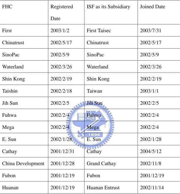
(11) study considers the restriction imposed by constant output in investigating the relationship between the market share and the efficiency score.. Blundell et al. (1999) point out that total industry profits decrease when more firms share the market.. The dominant firms tend to innovate more and industry. evolution is characterised by their persistent dominance.. In the securities industry,. investors at large discount brokerages using personal computer-based trading tend to trade more actively.. Barber and Odean (2001) have strongly suggested that there is a. link between the Internet and increased trading.. Guerrero et al. (2007) examine how. banks use Internet banking to lower costs and increase their income by attracting new customers and increasing sales to current customers.. The securities industry in Taiwan has become increasingly competitive, especially following the establishment of financial holding companies (FHCs) in 2003.. The regulatory authority in Taiwan has repeatedly encouraged domestic. financial institutions to form into FHCs.. The main purpose of forming an FHC is to. create bigger and stronger financial conglomerates that are capable of competing with international financial groups and gain a foothold on the worldwide financial market.. Accordingly, the Taiwan government enacted the Financial Holding. Company Act in 2001 and permitted only integrated securities firms (ISFs) to join as FHC’s subsidiaries.. As a consequence, law-induced FHCs in Taiwan provide the. opportunity to assess the impacts on the managerial efficiency of their securities subsidiaries.. Table 1-1 lists fourteen FHCs in Taiwan.. 2.

(12) TABLE 1-1. 14 FHCs Establishment in Taiwan FHC. Registered. ISF as its Subsidiary. Joined Date. Date First. 2003/1/2. First Taisec. 2003/7/31. Chinatrust. 2002/5/17. Chinatrust. 2002/5/17. SinoPac. 2002/5/9. SinoPac. 2002/5/9. Waterland. 2002/3/26. Waterland. 2002/3/26. Shin Kong. 2002/2/19. Shin Kong. 2002/2/19. Taishin. 2002/2/18. Taiwan. 2003/1/1. Jih Sun. 2002/2/5. Jih Sun. 2002/2/5. Fuhwa. 2002/2/4. Fuhwa. 2002/2/4. Mega. 2002/2/4. Mega. 2002/2/4. E. Sun. 2002/1/28. E. Sun. 2002/1/28. Cathay. 2001/12/31. Cathay. 2004/5/12. China Development. 2001/12/28. Grand Cathay. 2002/11/8. Fubon. 2001/12/19. Fubon. 2001/12/19. Huanan. 2001/12/19. Huanan Entrust. 2002/11/14. In other words, the environment in Taiwan is close to one with zero-sum gains (Lins et al., 2003) in which securities firms (SFs) expand their market share within a 100% constraint.. Tracy and Chen (2005) significantly improve existing data. envelopment analysis (DEA) models by providing a methodology for weight restrictions.. In addition, Lins et al. (2003) introduce a zero-sum gains data. envelopment analysis (ZSG-DEA) model, in which the sum of the outputs is. 3.

(13) constrained, in order to assess the ranking of participating countries in the Sydney 2000 Olympic Games based on single aggregated medals.. With these. developments in mind, this research proposes a framework to apply this ZSG-DEA model to the study of the securities industry that is based upon the maximisation of market share.. Since efficiency is an important topic in banking and finance, there have been numerous related studies (Camanho and Dyson, 2005; Chong et al., 2006; Drake and Hall, 2003; Drake et al., 2006).. However, very few studies have paid attention to the. securities industry’s efficiency.. There are still several important securities issues that. need to be further explored.. First, while market share is a frequently identified goal among market players, the literature seldom considers the pursuit of market share, and also neglects the zero-sum gains restriction.. The development of the performance evaluation under. zero-sum gains deserves further careful study.. This research therefore applies this. model of maximising the market share to analyse the competition among SFs in Taiwan.. Second, many studies use the DEA model to compute technical efficiency. However, empirical studies rarely investigate the relationship between the market share and the efficiency score.. The research thus studies the simultaneity between. the market share and the efficiency score using the two-stage least squares procedure (2SLS) proposed by Heckman (1978).. Martin (1979) indicates that advertising. intensity, seller concentration, and profitability are simultaneously determined. Brockett et al. (2004) recommend the use of simultaneous-equation estimation methods to examine the endogeneity of joint advertising and other variables in future 4.

(14) studies.. O’Brien (2002) employs 2SLS simultaneous equations systems to test. whether expenditures and votes are simultaneously determined.. Daneshvary and. Clauretie (2007) examine the effect of employer-provided health insurance on the annual earnings of married men and married women and account for the endogeneity of the health insurance decision using 2SLS.. Moreover, a comparison of the operating efficiency between foreign-affiliated and domestic SFs has seldom been empirically investigated.. In order to accelerate. the internationalisation and liberalisation of the domestic capital market, the Ministry of Finance in Taiwan launched ISFs in May 1988.. Foreign securities firms were. subsequently permitted to set up branches in Taiwan in 1989.. At the end of 2005, a. total of 11 foreign securities firms had set up branches in Taiwan.. Advanced. technology accompanies foreign direct investment entering the host country, thereby making foreign firms more efficient than their domestic competitors (Dimelis and Louri 2002).. Feinberg (2001) indicates that 94.1% of households use domestic. financial institutions as their primary provider of financial services in the U.S. Deyoung and Nolle (1996) find that foreign banks are less profit-efficient than U.S. banks.. This research also investigates the impact of a foreign ownership structure on. the efficiency score of SFs in a small open economy, namely, Taiwan.. We define the. foreign-affiliated SFs as those branches of multinational SFs in Taiwan since 1989, in contrast to the domestic SFs.. Meanwhile, the issue of whether or not FHCs parent companies can effectively improve an ISF’s managerial efficiency is still not empirically studied.. The lack of. firm-level data has made research on securities firms very difficult and rare to see (Goldberg et al., 1991), not to mention the effects of FHC on their managerial efficiency.. Drake et al. (2006) mention that little paper has been made in banking 5.

(15) sectors of the Fried et al. (1999) approach to adjusting inputs of DEA for incorporating with the impact of environmental factors.. This research also. investigates the influence of the law-induced FHC on its securities subsidiaries in terms of managerial efficiency.. 6.

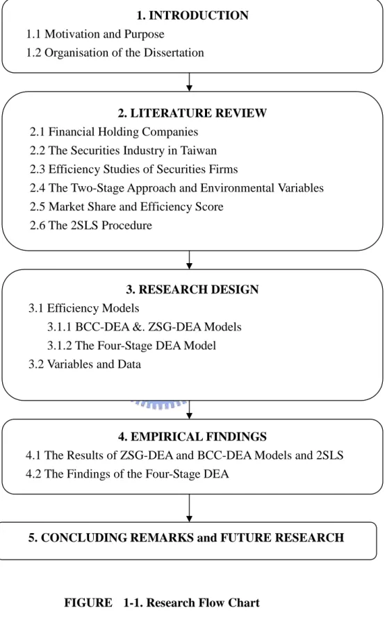
(16) 1.2 Organisation of the Dissertation The content and organisation of this dissertation summarize as follows:. 1.. Introduction: this section demonstrates the research motive and background, research purpose of the dissertation.. 2.. Literature Review: this section outlines the literature review of financial holding companies, securities industry in Taiwan, efficiency studies in securities firms, the two-stage data envelopment analysis method, the relationship between market share and efficiency score, and the 2SLS method.. 3.. Research Design: this section performs efficiency models and panel data descriptive.. 4.. Empirical Findings: this section demonstrates the research results of ZSG-DEA and BCC-DEA models, confirms the simultaneity between market share and efficiency score via the 2SLS, and presents the findings of the four-stage DEA model.. 5.. Conclusion, research limitation, and future research: this section presents the research limitation and plans future researches.. The research flow chart lists in Figure 1-1.. 7.

(17) 1. INTRODUCTION 1.1 Motivation and Purpose 1.2 Organisation of the Dissertation. 2. LITERATURE REVIEW 2.1 Financial Holding Companies 2.2 The Securities Industry in Taiwan 2.3 Efficiency Studies of Securities Firms 2.4 The Two-Stage Approach and Environmental Variables 2.5 Market Share and Efficiency Score 2.6 The 2SLS Procedure. 3. RESEARCH DESIGN 3.1 Efficiency Models 3.1.1 BCC-DEA &. ZSG-DEA Models 3.1.2 The Four-Stage DEA Model 3.2 Variables and Data. 4. EMPIRICAL FINDINGS 4.1 The Results of ZSG-DEA and BCC-DEA Models and 2SLS 4.2 The Findings of the Four-Stage DEA. 5. CONCLUDING REMARKS and FUTURE RESEARCH. FIGURE 1-1. Research Flow Chart. 8.

(18) 2. LITERATURE REVIEW This chapter demonstrates the literature review of financial holding companies, securities industry in Taiwan, efficiency studies in securities firms, the two-stage data envelopment analysis method, the relationship between market share and efficiency score, and the 2SLS method.. 2.1. Financial Holding Companies. Many economies encourage financial conglomeration and universal banking, including all European Union (EU) member countries and the United States.. In the. United States, the Gramm-Leach-Bliley Act on 12 November 1999 permitted single holding companies to offer banking, securities, and insurance (Barth et al., 2000). This new regulation is expected to accelerate the consolidation of the financial services industry.. In the EU, financial conglomerates and universal banking are. backdated to the 1989 Second Banking Directive, which was implemented earlier by all member economies.. Banks, investment firms, and insurance companies may. hold reciprocal equity participation, implying that there are no limits on the formation of financial conglomerates.. Following the progress of the European. Union and the United States, FHC is a newly arising organisational form in developing economies.. Some researchers have addressed the efficiency comparisons between financial conglomerates and specialised banks.. Vander Vennet (2002) analyses the cost and. profit efficiency of European financial conglomerate, universal banks, and specialised banks.. He further defines three main areas of financial services in the. EU: traditional banking, insurance, and securities-related activities.. 9. Financial.

(19) conglomerates are defined as financial services institutions that offer at least two of three main areas of financial services.. Universal banks are defined as diversified. banking firms that hold equity stakes in non-financial companies.. Operationally,. universal banks are those firms whose equity stakes in non-financial companies account for more than 1 % of total assets.. Furthermore, universal banks are. required to adhere to the criteria that the ratio of non-interest income to total revenues be higher than 5 %.. It is reported that financial conglomerates are more. revenue efficient than specialised banks, and the universal banks are both more cost and profit efficient than the non-universal banks.. Research on the effect of forced. mergers and acquisitions on the acquirer and the acquiring target is very limited. Chong et al. (2006) used an event study methodology to examine the impact of the forced merger scheme on the market-adjusted abnormal returns of Malaysian banks. That research shows that the forced merger mechanism destroys shareholders’ value. Contrary to the findings on voluntary mergers in the United States and Europe, Malaysian banks have a significantly negative cumulated abnormal return under the forced merger scheme.. The result further affirms that politics are often intertwined. with economic activities in less developed countries.. Steinherr and Huveneers (1994) also define that the key feature of universal banking is to hold equity shares of 5-20 % in other companies so as to monitor corporations as equity owner or to maintain a universal banking relationship.. Allen. and Gale (1995) define the relationship banks, such as the German, Dutch, and Swiss main banks, as providing both debt and equity financing to companies as well as establishing the long-lasting relationship with these companies. term for universal banks.. This is another. Benston (1994) also mentions that government regulators. have to regulate universal banks very tightly, hence hindering their economic 10.

(20) efficiency when considering the risk of financial instability.. From this viewpoint,. the smaller specialised banks have a number of advantages.. Because their. functions are limited, government agents can monitor them more efficiently.. Allen. and Rai (1996) divide countries into two groups, universal banking countries and separated banking countries, which prohibit the functional integration of commercial and investment banking.. That study shows that large banks in separated banking. countries have the largest measure of input inefficiency.. 2.2. The Securities Industry in Taiwan. Ashton (2001) mentions that many research studies in the USA and Europe have investigated the efficiency characteristics of banking. the efficiency score of securities firms. capital market.. Few studies address on. The securities industry is the centre of a. In Taiwan and in the UK, the stock market value to GDP is. approximately 140.. In addition, there is a higher turnover ratio in terms of trading. value for the Taiwan stock market compared to other major stock markets.. The. total trading amount in Taiwan’s securities market in 2006 achieved NT$24,205 billion including 98.7% in stocks (in dealing and brokerage), 0.12% in TDRs, 0.72% in warrants, 0.31% in ETFs, and 0.10% in others, respectively.. ISFs in Taiwan. perform various major services including brokerage activity, underwriting services, and proprietary trading.. The regulatory authority in Taiwan released the restriction. on the establishment of foreign-owned SFs in the mid of 1990s and introduced FHCs in 2003, but only allowing the ISFs to be a member of FHC.. The number of ISFs. increased from 39 in 1990 to 48 in 2006; the number of foreign-owned securities firms increased to 18 in 2006; the number of FHC-affiliated ISFs was 14 in 2006.. This shows that the Taiwan stock market is an important market to be 11.

(21) addressed as a research topic.. ISFs, which perform various major services. including investment banking, brokerage activity, underwriting services, and proprietary trading, are undergoing significant changes in Taiwan.. Except for. voluntary mergers in the market, financial groups have acquired many of the largest SFs including FHCs which have acquired them as one of their subsidiaries. Consequently, the top-14 market players account for 60 % of the total market share in the brokerage sector.. 2.3. Efficiency Studies of Securities Firms. Very limited knowledge is known about the efficiency score of the securities sector.. Goldberg et al. (1991) adopt survey data in a translog multi-product cost. function to examine the economies of scale and suggest that if the Glass-Steagall restrictions are relaxed, then banks can enter the securities industry with a brokerage division with about US$30 million in revenue.. The author reveals that cross-selling. activities between banks and securities are able to increase brokerage revenue.. Wang et al. (2003) use DEA and Tobit censored regression to assess the technical efficiencies of ISFs in Taiwan based on 1991-1993 data.. They conclude. that the impact of a firm’s service concentration on its technical efficiency is positive, which means that the diversity of services decreases its technical efficiency.. Firms. with branches have lower technical efficiencies than those without any branches, revealing that the purpose of setting up a new branch for an ISF is to enlarge the geographical coverage of the brokerage market.. When the stock market is. declining, having more branches instead becomes a burden for management and the increased complexities on operations make it difficult for managers to make decisions. 12.

(22) There are some research studies focusing on the relationship between specialisation and efficiency score.. Fung (2006) investigates the relationship. between scale efficiencies and X-efficiency for bank holding companies (BHCs) and indicated that a higher level of X-efficiency caused by more specialised banking activities might increase the efficiency scale.. Eaton (1995) and Wang et al. (1998). indicate that if firms dedicate themselves to one or two specialised businesses, then this helps create high efficiency score, because of the learning-curve effect.. Wang. and Yu (1995) investigate the economies of scope and economies of scale for ISFs in Taiwan.. Their study points out that the performances of ISFs are better than that of. specialised brokerage securities in terms of sales margin.. Wang and Yu also select. the ISF as their sample and concluded that when the number of branch offices increases, the ISF is in a diseconomy of scope.. Unlike the research concerning the impact of the parent holding company on its subsidiary being limited in amount, most studies have addressed the merger impact on the financial institutions.. Drake and Hall (2003) look at the technical efficiency. in Japanese banking incorporating problem loans under the large-scale merger wave. Their result suggests that larger banks operate well above the minimum efficiency scale and mergers have a limited opportunity to gain from eliminating X-inefficiencies.. If the efficiencies have more to do with specialisation, then the. trend towards enlargement and financial conglomeration in Japan may lead to decreasing levels of scale efficiency and X-efficiency.. On the contrary,. Worthington (2001) uses discrete choice regression models to investigate the influence of financial, managerial, and regulatory factors on the probability of a credit union merging during the period 1993-1995 and examines whether efficiency score has increased in these same institutions in the post-merger period 1996-1997. 13.

(23) The author adopts a Tobit censored regression model with a panel framework to analyse post-merger efficiency.. Mergers appear to have improved both on pure. technical efficiency and scale efficiency for the credit union industry.. Grabowski et. al. (1995) also conclude that the threat of takeovers serves as an efficiency enforcement mechanism in banks.. Fukuyama and Weber (1999) construct the. production technology and measure the cost efficiency score for Japanese SFs during 1988-1993 using a DEA model.. Wang et al. (2003) use the two-stage DEA. procedures to assess the technical efficiencies of integrated securities firms (ISFs) and conclude that the diversity of services decreases technical efficiency.. Zhang et. al. (2006) adopt a DEA approach to investigate the technological progress, efficiency score and productivity of the U.S. securities industry during 1980-2000 and report that smaller regional firms experience large decreases in both efficiency score and productivity.. Hence, this research examines the technical efficiency of top-14 ISFs. and then investigates the threat from FHC imposed upon ISF’s managerial efficiency.. 2.4. The Two-stage Approach and Environmental Variables The two-stage approach (McCarty and Yaisawarng, 1993; Wang et al., 2003) involves solving a DEA problem in the first stage and then the efficiency score obtained in the first stage being regressed upon the environmental variables in the second stage.. Some factors, which are environmental variables, may affect the. efficiency score of DMUs.. The sign of the coefficients of the environmental. variables indicates the direction of the influence, and the standard hypothesis tests can be used to measure the strength of the relationship. Researchers adopt the Tobit. regression model instead of the OLS model to measure the significance of the relationship.. Esho (2001) adopts the second-stage regression to investigate the. relationship between the capital to asset ratio, size, age, and efficiency score. 14.

(24) Mukherjee et al. (2001) investigate the relationships between the asset value, the square of asset value, and productivity growth and find out that the bigger-sized American banks have significantly positive influences on productivity growth, but insignificant coefficients on the square of asset value.. Dimelis and Louri (2002). analyse the efficiency gains caused by the diverse degree of foreign ownership in Greece in 1997 which indicate a positive effect on labour productivity of foreign ownership.. Deyoung and Nolle (1996) find out that foreign-owned banks are less. profit-efficient than U.S.–owned banks.. Elyasiani and Mehdian (1997) report that. foreign-owned banks are less cost efficient than U.S. bank and even statistically insignificant.. Wheelock and Wilson (2000) include a dummy variable to test. whether membership in a multi-bank holding company affects the probability of failure.. These authors indicate that if a parent company injects cash into a weak. subsidiary, than a holding company membership might lessen the chance of failure. On the other hand, the failure of a primary bank in a holding company has sometimes led regulators to close all holding company members.. It is an interesting issue of. this research to investigate whether the efficiency score of foreign-owned securities firms or members of FHCs is better than that of the domestic specialised securities firms or not.. 2.5. Market Share and Efficiency Score Firms focus on market share in order to increase shareholder value through improved efficiency score, thereby benefiting consumers.. Goldberg and Rai (1996),. Smirlock (1985), Peltzman (1977) and Demsetz (1973) note the correlation between market share and profitability.. Hannan (1991) considers the greater efficiency. score of firms with larger market shares to be a source of the positive relationship between profits and concentration.. Goldberg and Rai (1996) develop the 15.

(25) efficient-structure (EFS) hypothesis which suggests that efficient firms increase in terms of their size and market share due to their ability to generate higher profits, thus leading to a higher degree of market concentration.. Smirlock (1985) includes. market share as an independent variable that is positively and significantly related to profitability even after controlling for concentration.. However, Goldberg and Rai. (1996) and Shepherd (1986) indicate that the conclusion depends on whether market share can be regarded as a proxy for the efficiency score of larger firms rather than as a measure of their market power.. Martin (1988) shows how larger firms have. lower costs due to the economies of scale in their industries or because of their inherent superiority within their respective industries.. The larger firms have. price-cost margin advantages over their smaller rivals.. Based on the above. literature, this study considers the restriction imposed by constant output in investigating the relationship between the market share and the efficiency score.. Blundell et al. (1999) point out that total industry profits decrease when more firms share the market.. The dominant firms tend to innovate more and industry. evolution is characterised by their persistent dominance.. 2.6. The Two-Stage Least Squares Procedure (2SLS). The two-stage least squares procedure (2SLS) was proposed by Heckman (1978).. Martin (1979) indicates that advertising intensity, seller concentration, and. profitability are simultaneously determined.. Brockett et al. (2004) recommend the. use of simultaneous-equation estimation methods to examine the endogeneity of joint advertising and other variables in future studies.. O’Brien (2002) employs the. 2SLS approach to test whether expenditures and votes are simultaneously determined.. Daneshvary. and. Clauretie 16. (2007). examine. the. effect. of.

(26) employer-provided health insurance on the annual earnings of married men and married women and account for the endogeneity of the health insurance decision using 2SLS.. 17.

(27) 3. RESEARCH DESIGN Avkiran (1999) employs two DEA models to measure the efficiency score and indicates that DEA analysis is sensitive to the choice of variables.. However, this is. also a kind of strength in providing management-specific information as the method for improving firm-level efficiency score.. Efficiency measurement using DEA. models from different perspectives can depend on the decision-making requirements.. 3.1. Efficiency Models 3.1.1. Traditional BCC-DEA and Zero-Sum Gains DEA Methodology. DEA is a linear programming model that identifies an efficient frontier, which consists of efficient decision-making units (DMUs).. Efficient DMUs are those units. for which no other DMUs are able to generate at least the same amount of each output under given inputs (Charnes et al., 1978).. The efficiency score reflects the ability of. firms to generate the maximum outputs under a given level of inputs.. 3.1.1.1 Traditional BCC-DEA Model. DMUi represents the object unit that is attempting to maximise its output. All DMUs in the same year constitute the reference set used to construct the efficiency frontier for each DMUi.. The aim of the traditional DEA model is to make the less. efficient object unit at least as efficient as the others by increasing its output.. For. each DMUi the efficiency score (i) is obtained from a measure of the ratio of all outputs over all inputs. Charnes et al. (1978) develop the constant-returns-to-scale (CRS) DEA model as below:. 18.

(28) M. i  Max. u m 1 K. m m i. y. v x k 1. k k i. (1). M. u m 1 K. s.t.. m. y. v x k 1. k. m j.  1, j  1,..., N. k j. um , vk  0, m  1,..., M , k  1,..., K where i is the efficiency score of DMUi; xjk, yjm >0 represent input and output data for the j-th DMU with the ranges for j, k, and m indicated in (1); N is the number of DMUs; xjk is the amount of the k-th input consumed by the j-th DMU; yjm is the amount of the m-th output produced by the j-th DMU; and um and vk are output and input weights assigned to the m-th output and the k-th input, respectively. One problem with this above ratio form is that the number of solutions is infinite - e.g., if (um* , vk* ) is a solution, then (cum* , cvk* ) is another solution, where c is a constant.. In order to avoid this problem, an output-oriented DEA model, which is to. achieve the efficient DMU by a radial expansion in outputs, can impose the constraint M. u m 1. m. y mj  1 , which provides: K. Min vk x kj k 1. M. s.t.. u m 1. m. y mj  1. K. M. k 1. m 1. (2).  vk x kj   um y mj  0, j  1,..., N um , vk  0, m  1,..., M , k  1,..., K. Banker et al. (1984) extend the constant returns to scale (CRS) DEA model to a variable returns to scale (VRS) situation.. The dual solution of the traditional. output-oriented BCC-DEA model using duality expressed by Coelli et al. (2005) to 19.

(29) measure the efficiency score i for DMUi is shown as: 1  Max  i i. i , 1 ,..., N N. s.t.. i yim    j y mj , m  1,..., M , j 1. (3). N. xik    j x kj , k  1,..., K , j 1. N.  j 1. j.  1,. 1 ,..., N  0 where i depicts the inverse of the efficiency score of DMUi; the efficiency score i of DMUi is 1/i; N is the number of DMUs; K and M are, respectively, the numbers of inputs and outputs; xjk is the amount of the k-th input consumed by the j-th DMU; yjm is the amount of the m-th output produced by the j-th DMU; and j is each efficient DMU’s individual share in the definition of the target for DMUi. The BCC-DEA model here measures the firm-level efficiency score (i) in the securities industry.. An SF (as a DMU in the DEA model) that is pursuing more. market share naturally means that other SFs lose some market share, because the total market share is 100%.. Accordingly, this constant sum of output is unable to use the. traditional BCC-DEA model, in which the output of any given DMU is not influenced by the output of the others, to assess the efficiency score.. This is our motivation for. adopting the ZSG-DEA model to measure the efficiency scores of SFs.. 3.1.1.2 Zero-Sum Gains DEA Model. The ZSG-DEA model assesses the efficiency score provided that the sum of outputs is constant.. Lins et al. (2003) indicate that this is similar to a zero-sum game. whereby how much is won by a player is lost by one or more of the other players. The equal output reduction strategy is generated to measure the efficiency score 20.

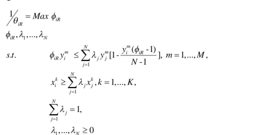
(30) ( iR  1 ) for DMUi in equation (4) using duality expressed shown below and is iR graphically represented using a simple case involving one input, x, and one output, y, in Figure 3-1: 1  Max  iR iR. iR , 1 ,..., N N. iR yim    j y mj [1-. s.t.. j 1. yim (iR -1) ], m  1,..., M , N -1 (4). N. x    j x , k  1,..., K , k i. j 1. N.  j 1. j. k j.  1,. 1 ,..., N  0 where the term iR is the inverse of the efficiency score of the ZSG-DEA model with. iR  1; and the efficiency score iR of DMUi is the inverse of iR (iR =1/iR) in the ZSG-DEA model.. The term yim (iR -1) , representing losses of the other DMUj (j ≠. i), must have one DMUi to gain yim (iR -1) output units.. y. BCC-DEA Model. ZSG-DEA Model. yi (iR -1). i yi.  iR y i yi. x FIGURE 3-1. Graphical Representation of the Equal Output Reduction Method. 21.

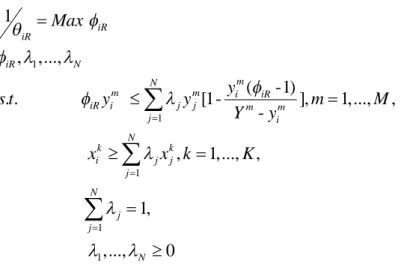
(31) This model here causes some DMUs to have a negative output after replacing the output as the reduction coefficient.. A simple example in Appendix A illustrates. an unreasonable case in which an equal output reduction under a zero-sum game generates. a. negative. output.. Hence,. provided. that. yim (iR -1)  min ( y mj ), m  1,..., M , this equal output reduction strategy can apply. To avoid this major weakness, Lins et al. (2003) further develop the proportional yim (iR -1) output reduction strategy for any given DMUi using the ratio , where Y m m m Y - yi is the constant sum of the m-th output.. Thus, DMUi needs to win yim (iR -1) output. units, and the losses of the other DMUs are proportional to their levels of output. The condition that the sum of the losses is equal to the gains of DMUi still holds. Figure 3-2 represents the ZSG-DEA frontier created by this proportional reduction strategy and the BCC-DEA frontier using a simple case involving one input and one output.. DMUi gains yim (iR -1) output units, and the losses of other DMUs. yim (iR -1) are proportional to their respective levels of output, which is y ( m m ) . Y - yi m j. If the. output yj of DMUj is larger than those of other DMUs, then the output reduction y mj (. yim (iR -1) ) is also larger than those of the others, and vice versa. Y m - yim. Model (5). substitutes model (4) for the proportional output reduction strategy in measuring the efficiency score ( iR  1 ) of DMUi as: iR. 22.

(32) 1  Max  iR iR. iR , 1 ,..., N N. s.t.. iR yim    j y mj [1j 1. yim (iR -1) ], m  1,..., M , Y m - yim (5). N. xik    j x kj , k  1,..., K , j 1. N.  j 1. j.  1,. 1 ,..., N  0 However, Lins et al. (2003) report that obtaining results based on this non-linear programming problem is very labour-consuming in particular because of the large number of variables. =1).. The model is thus simplified by having only a single output (m. Appendix A provides an example to explain the computational steps of the. proportional output reduction strategy.. y. BCC-DEA Model ZSG-DEA Model. yi (iR -1). iR yi. i yi yi. x FIGURE 3-2. Graphical Representation of the Proportional Output Reduction Method The following theorem holds under a single output ZSG-DEA proportional reduction strategy: LGSS Theorem (Lins et al., 2003).. The target for a DMU to reach the efficiency 23.

(33) frontier in a ZSG-DEA proportional output reduction strategy model equals the same target in the traditional BCC-DEA model multiplied by the reduction coefficient (1yi (iR -1) ). Y - yi. Owing to this theorem, equation (6) below holds.. iR yi . N.   y [1j 1. j. j. yi (iR -1) ] Y - yi. (6). y ( -1)  i yi [1- i iR ] Y - yi. The efficiency score of the ZSG-DEA model is obtained from equation (7):. iR. i yi (Y - yi )  yi 2  yi (Y - yi  1). (7). In this research, due to the fact that the sum of the total market share in percentage terms is 100, Y is always 100 and equation (7) above can be expressed as equation (8):. iR. i yi (100 - yi )  yi 2  yi (100 - yi  1). (8). Lins et al. (2003) also infer that the value of the weight of DMUi’s peers (i) equals its value in the traditional BCC-DEA model.. This ZSG-DEA model is then. applied to measure the efficiency score of SFs when the market share in percentage terms always sums up to 100.. 3.1.2. The Four-Stage DEA Technical efficiency reflects the ability of firms to use as little input as possible to obtain a given level of output.. Fried et al. (1999) introduce a four-stage DEA.. The management component of inefficiency is separated from the influences of the external environment as the management level is not able to control these influences. The result is a radial measurement of managerial efficiency. 24. The managerial.

(34) efficiency is the efficiency score purged of the influences of the external environments, as the management level are not able to control these influences, indeed the assessment of managerial competence on running a business.. The first stage calculates a DEA frontier using the observable inputs and outputs according to the variable returns to scale (VRS) model.. Charnes et al. (1978) propose. an input-oriented model and assume constant returns to scale (CRS) as follows: Min. i. i , 1 ,..., N N. s.t.. -yim +  j y mj  0, m  1,..., M , j 1. (9). N.  x    j x  0, k  1,..., K , k i i. j 1. k j. 1 ,..., N  0. where i is the technical efficiency (TE) of DMUi ; N is the number of ISF; K and M are respectively the number of inputs and outputs; xik is the amount of the k-th input consumed by the i-th ISF; yim is the amount of the m-th output produced by the i-th ISF; and j is a scalar value representing a proportional contraction of all inputs, holding input ratios and output level constant.. Banker et al. (1984) extend the CRS DEA model to account for a VRS situation. The CRS linear programming problem can be easily added onto the equation and modified to be the VRS model as below:. 25.

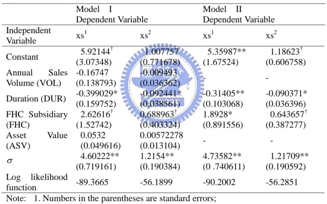
(35) i. Min. i , 1 ,..., N N. -yim +  j y mj  0, m  1,..., M ,. s.t.. j 1. N. (10). i xik    j x kj  0, k  1,..., K , j 1. N.  j 1. j.  1,. 1 ,..., N  0 where i is the pure technical efficiency (PTE) of DMUi.. TE is the ability of. management to implement a technically efficient production plan (Berger et al., 1993): TEi  PTEi  SEi. (11). where SE i is the scale efficiency index for DMUi in a period.. That is, technical. efficiency is decomposed into pure technical efficiency and scale efficiency (Banker et al., 1984; Fung, 2006).. If there is a difference in the TE and PTE scores for the. i-th DMU, then this indicates that the firms have scale inefficiency.. The radial. technical efficiency scores, input slacks, and output surplus are computed for each observation (Farrell, 1957).. The DEA has been applied in activities of a very diverse nature such as: public health (hospitals, clinics), education (schools, universities), banks, factories, fast food restaurants, etc. securities firms.. Few papers use DEA to study the efficiency score of. Here we adopt the VRS-DEA to compute the securities firms’. input slacks.. The second stage estimates the K input equations using a Tobit censored regression.. The dependant variables are radial plus slack input movement; the. 26.

(36) independent variables are measures of environmental variables applicable to the particular input.. The objective is to quantify the effect of external conditions on the. excessive use of inputs.. The K equations are specified as:. xsik  f k ( Eik ,  k , uik ); i  1,..., N ; k  1 ,..., K. (12). where xsik is the total radial plus slack movement for input k of ISF I based on the DEA results from stage 1; Eik is a vector of variables characterizing the operating environment for ISF i that may affect the utilization of input; k is a vector of coefficient and uik is a disturbance term.. Here, we adopt both continuous and. categorical variables as regressors.. The third stage uses the estimated coefficients from the above-mentioned equations to predict total input slack for each ISF based on its environmental variables: xsik  f k ( Eik ,  k ); i  1,..., N ; k  1 ,..., K. (13). These predictions are used to adjust the primary input data for each ISF based on the difference between maximum predicted total input slack and predicted total input slack: ^. xik adj  xik  [ Max k {xsik }  E ( xsik | Eik )]; i  1,..., N ; k  1 ,..., K. (14). This generates a new projected dataset where the inputs are adjusted for the influence of external conditions.. The final stage uses the adjusted dataset to re-compute the DEA model under the. 27.

(37) initial output data and adjusted input data. measures of inefficiency.. The result generates new radial and slack. These radial and slack scores measure the inefficiency that. is attributable to management that is wholly managerial inefficiency.. 3.2. Variables and Data. 3.2.1 Variables This research follows the model developed by Lins et al. (2003) in that it chooses a single output and multiple inputs to measure the efficiency score.. Drake. et al. (2006) introduce a profit-oriented model with revenue components as outputs and cost components as inputs in a banking efficiency study.. Banks pursue their. profit maximisation goal by increasing revenue and reducing cost.. In the securities. industry, an individual SF pursues the goal of market share maximisation by innovating itself as an e-broker or e-trader.. Thus, this output-oriented ZSG-DEA. model chooses market share as the single output.. Drake and Hall (2003) adopt. general and administrative expenses and fixed assets as the two inputs of the DEA model.. Berger and Mester (1997) indicate that another important aspect of. efficiency measurement is the treatment of financial capital.. A bank’s financial. capital that is available to absorb possible losses helps reduce its insolvency risk. Accordingly, the study adopts fixed assets, in which the SFs increase their fixed assets by investing in computer hardware, financial capital as well as general and administrative expenses as the three inputs of the ZSG-DEA model. 3.2.2 Data A panel dataset covering the period 2001-2005 includes 266 ISFs in Taiwan. During 2002, eight SFs were merged and one foreign-affiliated SF established branches in Taiwan.. In 2003, four SFs were merged and one foreign-affiliated 28.

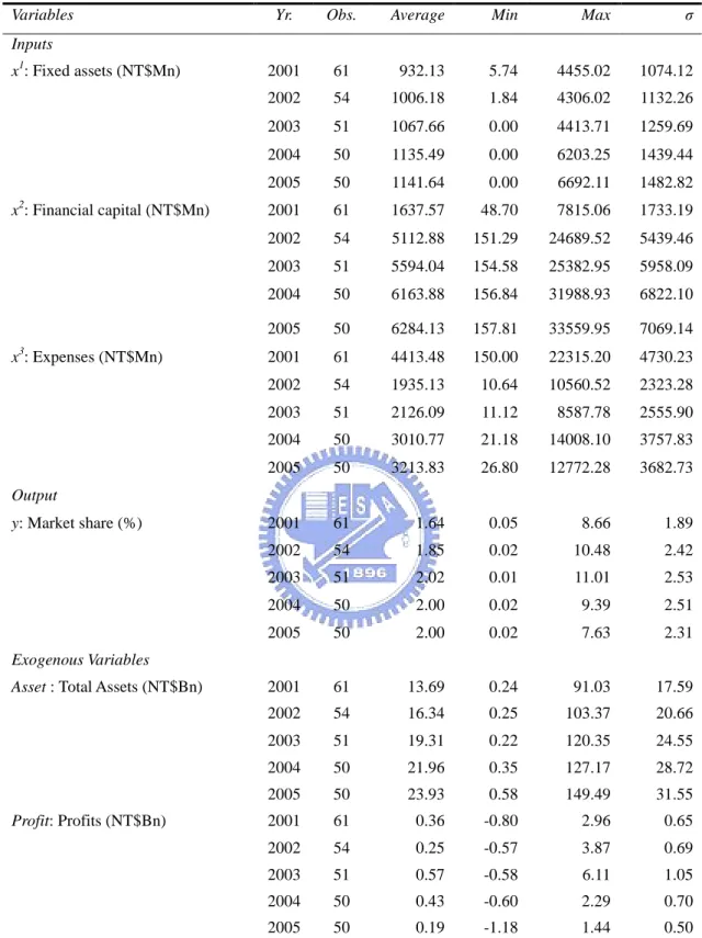
(38) institution joined the securities market in Taiwan. observations from 2001-2005.. Appendix B lists the number of. Since the data cover five years, several variables,. including three inputs, which are exogenous variables in the 2SLS, are deflated with the gross domestic product (GDP) deflator (2001=100) to avoid the distortion caused by inflation (Bierlen and Featherstone, 1998; Li et al., 2004).. Market share is the. trading amount in brokerage and proprietary trading of an individual firm divided by the total trading amount of all securities’ brokers and dealers.. The firm-level data for. the exogenous variables in the 2SLS are the trading amounts, fixed assets, general expenses, financial capital, total assets, and profits.. All variable data are obtained. from the reports of the Taiwan Stock Exchange Corporation during the 2001-2005 period. (http://www.tse.com.tw/ch/statistics/statistics_list.php?tm=03&stm=004,. accessed April 4, 2007).. The descriptive statistics for all the variables are shown in. Table 3-1.. 29.

(39) TABLE 3-1. Descriptive Statistics for the BCC-DEA, ZSG-DEA and 2SLS Variables. Yr.. Obs.. Average. Min. Max. σ. 2001. 61. 932.13. 5.74. 4455.02. 1074.12. 2002. 54. 1006.18. 1.84. 4306.02. 1132.26. 2003. 51. 1067.66. 0.00. 4413.71. 1259.69. 2004. 50. 1135.49. 0.00. 6203.25. 1439.44. 2005. 50. 1141.64. 0.00. 6692.11. 1482.82. 2001. 61. 1637.57. 48.70. 7815.06. 1733.19. 2002. 54. 5112.88. 151.29. 24689.52. 5439.46. 2003. 51. 5594.04. 154.58. 25382.95. 5958.09. 2004. 50. 6163.88. 156.84. 31988.93. 6822.10. 2005. 50. 6284.13. 157.81. 33559.95. 7069.14. 2001. 61. 4413.48. 150.00. 22315.20. 4730.23. 2002. 54. 1935.13. 10.64. 10560.52. 2323.28. 2003. 51. 2126.09. 11.12. 8587.78. 2555.90. 2004. 50. 3010.77. 21.18. 14008.10. 3757.83. 2005. 50. 3213.83. 26.80. 12772.28. 3682.73. 2001. 61. 1.64. 0.05. 8.66. 1.89. 2002. 54. 1.85. 0.02. 10.48. 2.42. 2003. 51. 2.02. 0.01. 11.01. 2.53. 2004. 50. 2.00. 0.02. 9.39. 2.51. 2005. 50. 2.00. 0.02. 7.63. 2.31. 2001. 61. 13.69. 0.24. 91.03. 17.59. 2002. 54. 16.34. 0.25. 103.37. 20.66. 2003. 51. 19.31. 0.22. 120.35. 24.55. 2004. 50. 21.96. 0.35. 127.17. 28.72. 2005. 50. 23.93. 0.58. 149.49. 31.55. 2001. 61. 0.36. -0.80. 2.96. 0.65. 2002. 54. 0.25. -0.57. 3.87. 0.69. 2003. 51. 0.57. -0.58. 6.11. 1.05. 2004. 50. 0.43. -0.60. 2.29. 0.70. 2005. 50. 0.19. -1.18. 1.44. 0.50. Inputs x1: Fixed assets (NT$Mn). 2. x : Financial capital (NT$Mn). 3. x : Expenses (NT$Mn). Output y: Market share (%). Exogenous Variables Asset : Total Assets (NT$Bn). Profit: Profits (NT$Bn). Note:. 1. Variables are deflated with the gross domestic product (GDP) deflator (2001=100) to avoid the distortion caused by inflation. 2. Data Sources: Taiwan Stock Exchange Corporation (Website: http://www.tse.com.tw/ch/statistics/statistics_list.php?tm=03&stm=004).. We furthermore construct a panel dataset during 2002-2005 of the top twelve to 30.

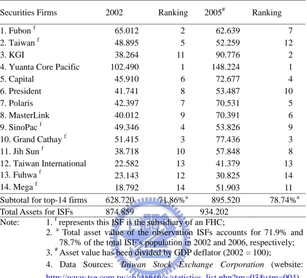
(40) fourteen securities firms in Taiwan.. The firm-specific financial data are collected. from peers’ data exchange among the securities firms and the reports of the Taiwan Stock. Exchange. Corporation. (Website:. http://www.tse.com.tw/ch/statistics/statistics_list.php?tm=03&stm=004).. For the. fiscal year of 2002, some of these ISFs were committed themselves as an FHC’s subsidiary in 2003.. This period offers to measure the technical efficiency and. managerial efficiency before imposing the impact of FHC. treated as a DMU under the DEA model. the number of DMUs.. Each of these ISFs is. Two guidelines are commonly applied on. One is that the total number of inputs and outputs should be. less than one third that the number of DMUs in the DEA model. (Friedman and Sinuany-Stern, 1998). Another is that the number of DMUs should be at least two. times the number of inputs multiplied by the number of outputs (Dyson et al., 2001). In our model there are two inputs and two outputs.. The number of DMUs in a year. is hence more than triple the total number of input and output items.. In order to increase the homogeneity of DMUs, the ISFs with the top twelve to fourteen asset values are selected.. As Table 3-2 shows, these selected ISFs account. for more than 70 percent of the total assets of the entire ISF sectors in Taiwan.. 31.

(41) TABLE 3-2. The Asset Value (NT$Bn) of Top-14 ISFs in Taiwan Securities Firms. 2002. Ranking. 2005#. Ranking. 1. Fubon f 65.012 2 62.639 7 f 2. Taiwan 48.895 5 52.259 12 3. KGI 38.264 11 90.776 2 4. Yuanta Core Pacific 102.490 1 148.224 1 5. Capital 45.910 6 72.677 4 6. President 41.741 8 53.487 10 7. Polaris 42.397 7 70.531 5 8. MasterLink 40.012 9 70.391 6 f 9. SinoPac 49.346 4 53.826 9 f 10. Grand Cathay 51.415 3 77.436 3 f 11. Jih Sun 38.718 10 57.848 8 12. Taiwan International 22.582 13 41.379 13 f 13. Fuhwa 23.143 12 30.825 14 f 14. Mega 18.792 14 51.903 11 a Subtotal for top-14 firms 628.720 71.86% 895.520 78.74%a Total Assets for ISFs 874.859 934.202 Note: 1. f represents this ISF is the subsidiary of an FHC; 2. a Total asset value of the observation ISFs accounts for 71.9% and 78.7% of the total ISF’s population in 2002 and 2006, respectively; # 3. Asset value has been divided by GDP deflator (2002 = 100); 4. Data Sources: Taiwan Stock Exchange Corporation (website: http://www.tse.com.tw/ch/statistics/statistics_list.php?tm=03&stm=004). The top twelve ISFs have exchanged data such as market share and brokerage revenue for peer comparison since 2001.. Fuhwa Securities and Mega Securities did. not exchange financial data with peers due to the smaller assets of Mega and unavailable data of Fuhwa in 2002.. Mega Securities merged with another ISF to. increase its asset by almost triple compared with its assets in 2002.. Two more ISFs. joined the exchange pool in 2003, making fourteen securities firms available for DEA.. The top twelve ISFs have exchanged data such as market share and brokerage revenue for peer comparison since 2001.. Fuhwa ISF and Mega ISF did not. exchange financial data with peers due to the smaller assets of Mega and unavailable. 32.

(42) data of Fuhwa in 2002.. Mega ISF merged with another ISF to increase its asset by. almost triple compared with its assets in 2002.. Two more ISFs joined the exchange. pool in 2003, making fourteen securities firms available for DEA.. This study further employs a profit-oriented, non-parametric model, which uses revenue components as outputs, and cost components as inputs.. Drake et al. (2006). use this profit-oriented DEA model to investigate the bank efficiency in Hong Kong.. The first stage input-oriented DEA model includes physical inputs and outputs in the strict production theory sense.. There are two outputs: market share of. brokerage business (MS) and revenue (BR), which includes the fee income and service charge in the brokerage business.. The market share of the brokerage business is an. important factor to evaluate performance for senior managers.. This research is the. first one to introduce market share as an output to evaluate an ISF’s efficiency score. Revenue from the brokerage business accounts for roughly 70 % of total revenue of the top-10 Taiwanese Securities firms.. Revenue from the brokerage business as an. output is shown on the existing literature.. Two inputs are used to produce brokerage services: branches (BO) and the discounted expense amount of the brokerage business (DE). divided by GDP deflator (2002 = 100). explanation of variables.. 33. BR and DE have been. Table 3-3 presents the definition and.

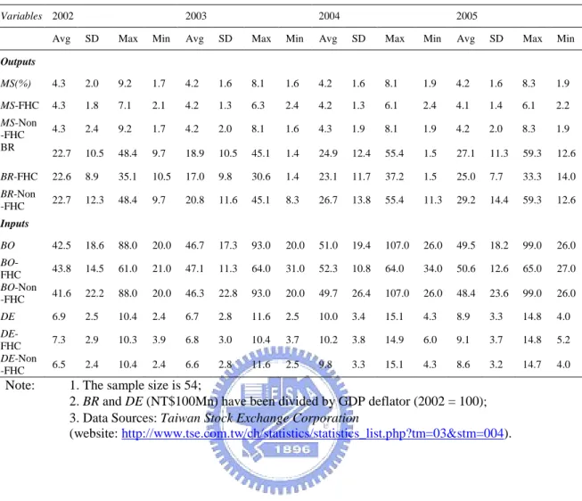
(43) TABLE 3-3. Definition and Explanation of Variables for the Four-Stage DEA Variable. Definition. MS = y1. Market share for brokerage business (%). BR = y2. Brokerage revenue (NT$100Mn). BO = x1. Branch offices. DE = x2. Discounted expenses (NT$100Mn). Goldberg et al. (1991) also adopted branch office as one of the inputs in the literature.. In practice, high discounted expenses provide benefits to customers.. When the discounted amount is more, then it motivates customers to trade equities with this ISF.. It also benefits the broker’s market share.. This research is the first. one to adopt the discounted expense amount as one input for research. of the brokerage business is measured in percentage terms.. Brokerage revenue and. the discounted expenses are measured in NT$100 million. descriptive statistics of the raw data.. 34. Market share. Table 3-4 displays.

(44) TABLE 3-4. Descriptive Statistics of ISFs for the Four-Stage DEA Variables 2002. 2003. 2004. 2005. Avg. SD. Max. Min. Avg. SD. Max. Min. Avg. SD. Max. Min. Avg. SD. Max. Min. MS(%). 4.3. 2.0. 9.2. 1.7. 4.2. 1.6. 8.1. 1.6. 4.2. 1.6. 8.1. 1.9. 4.2. 1.6. 8.3. 1.9. MS-FHC. 4.3. 1.8. 7.1. 2.1. 4.2. 1.3. 6.3. 2.4. 4.2. 1.3. 6.1. 2.4. 4.1. 1.4. 6.1. 2.2. 4.3. 2.4. 9.2. 1.7. 4.2. 2.0. 8.1. 1.6. 4.3. 1.9. 8.1. 1.9. 4.2. 2.0. 8.3. 1.9. 22.7. 10.5. 48.4. 9.7. 18.9. 10.5. 45.1. 1.4. 24.9. 12.4. 55.4. 1.5. 27.1. 11.3. 59.3. 12.6. BR-FHC. 22.6. 8.9. 35.1. 10.5. 17.0. 9.8. 30.6. 1.4. 23.1. 11.7. 37.2. 1.5. 25.0. 7.7. 33.3. 14.0. BR-Non -FHC. 22.7. 12.3. 48.4. 9.7. 20.8. 11.6. 45.1. 8.3. 26.7. 13.8. 55.4. 11.3. 29.2. 14.4. 59.3. 12.6. 42.5. 18.6. 88.0. 20.0. 46.7. 17.3. 93.0. 20.0. 51.0. 19.4. 107.0. 26.0. 49.5. 18.2. 99.0. 26.0. 43.8. 14.5. 61.0. 21.0. 47.1. 11.3. 64.0. 31.0. 52.3. 10.8. 64.0. 34.0. 50.6. 12.6. 65.0. 27.0. 41.6. 22.2. 88.0. 20.0. 46.3. 22.8. 93.0. 20.0. 49.7. 26.4. 107.0. 26.0. 48.4. 23.6. 99.0. 26.0. 6.9. 2.5. 10.4. 2.4. 6.7. 2.8. 11.6. 2.5. 10.0. 3.4. 15.1. 4.3. 8.9. 3.3. 14.8. 4.0. 7.3. 2.9. 10.3. 3.9. 6.8. 3.0. 10.4. 3.7. 10.2. 3.8. 14.9. 6.0. 9.1. 3.7. 14.8. 5.2. 6.5. 2.4. 10.4. 2.4. 6.6. 2.8. 11.6. 2.5. 9.8. 3.3. 15.1. 4.3. 8.6. 3.2. 14.7. 4.0. Outputs. MS-Non -FHC BR. Inputs BO BOFHC BO-Non -FHC DE DEFHC DE-Non -FHC. Note:. 1. The sample size is 54; 2. BR and DE (NT$100Mn) have been divided by GDP deflator (2002 = 100); 3. Data Sources: Taiwan Stock Exchange Corporation (website: http://www.tse.com.tw/ch/statistics/statistics_list.php?tm=03&stm=004).. Four environmental variables are introduced to measure the effect of input utilization.. Annual sales volume is the exchanged data among the top-14 ISFs.. Durations are calculated by each firm’s registration date in the Taiwan Market Post Information System and asset values are the annual report data listed in the Taiwan Securities and Futures Bureau.. 35.

(45) 4. EMPIRICAL RESULTS This chapter demonstrates the research results of ZSG-DEA and BCC-DEA models, confirms the simultaneity between market share and efficiency score via the 2SLS, and the findings of the four-stage DEA model.. 4.1. The Result of ZSG-DEA, BCC-DEA Models and 2SLS Procedure. Section 4.1.1 analyses the result of ZSG-DEA and traditional DEA models. Section 4.1.2 confirms the simultaneous relationship between market share and efficiency score via 2SLS. 4.1.1. Examining the Results of the ZSG-DEA and BCC-DEA Models. This research adopts the output-oriented variable-returns-to-scale BCC-DEA model (Banker et al., 1984) and the ZSG-DEA model (Lins et al., 2003) to compute the efficiency scores of the SFs.. Output orientation is a better choice here because. the obvious aim of an individual SF is to obtain the maximum market share in order to dominate the market.. The securities industry in Taiwan provides an opportunity to. apply the ZSG-DEA model, because of its characteristics of high competition and low concentration (the top-three banks’ concentration ratios, CR3, were all less than 0.3 during 2001-2005).. Market share is the most important performance indicator. among the securities firms. Equations (3) and (8) calculate the efficiency scores i and iR from the BCC-DEA and ZSG-DEA models using the annual cross-sectional data, respectively, which are presented in Appendix B.. It is obvious that when faced with the reality of. 36.

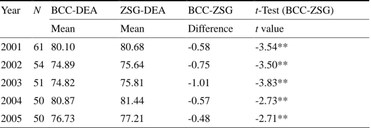
(46) a constant sum of outputs, the traditional BCC-DEA model underestimates the average efficiency score compared with the ZSG-DEA model.. This study calculates. a paired-difference t test to determine whether the efficiency scores of these two models are significantly different.. Table 4-1 presents the results of the paired t test.. The efficiency scores (iR) in the ZSG-DEA model are statistically significantly higher than those (i) in the BCC-DEA model during 2001-2005.. The gap in. efficiency scores between the efficient and inefficient SFs under a zero-sum gains framework is significantly less than that under the traditional models.. Hence, with. the objective of maximising their market share, the efficient SFs need to develop more marketing strategies and introduce more techniques to maintain their leading role in the market.. We are also able to derive this trend in the descriptive statistics.. The. average fixed assets of (x1) and financial capital (x2) in 2005 respectively increased by 23% and by more than three times the value in 2001, showing that the SFs continuously enhance their capital and fixed assets to develop electronic trading hardware to maximise their market shares.. The average expenses in 2005 were also. nearly 30% lower than the corresponding values in 2001.. However, the average. market share of SFs in 2005 reflected an increase of only 22% compared with the value in 2001.. Owing to the fact that the market share competition is like a. zero-sum constraint, the severe competition resulted in each SF obtaining a higher efficiency score under the ZSG-DEA model than under the BCC-DEA model.. 37.

(47) TABLE 4-1. Tests of the Efficiency Differences between the BCC-DEA and ZSG-DEA Year. N BCC-DEA. ZSG-DEA. BCC-ZSG. t-Test (BCC-ZSG). Mean. Mean. Difference. t value. 2001. 61 80.10. 80.68. -0.58. -3.54**. 2002. 54 74.89. 75.64. -0.75. -3.50**. 2003. 51 74.82. 75.81. -1.01. -3.83**. 2004. 50 80.87. 81.44. -0.57. -2.73**. 2005. 50 76.73. 77.21. -0.48. -2.71**. Notes: 1. Eight SFs were merged and one Hong Kong-based SF established its Taiwan branch in 2002; 2. Four securities firms were merged and one American-based SF was established in 2003; 3. ** indicates significance at the 1% level; 4. Shapiro-Wilk W test is verified for examining the normality of the data. 4.1.2. Simultaneous Relationship between Market Share and Efficiency Score. The EFS hypothesis states that efficient firms increase in size and market share due to their ability to generate higher profits (Goldberg and Rai, 1996).. Martin. (1988) indicates that larger firms have lower costs, either because of the economies of scale in their industries or due to the inherent superiority of the larger firms in their industries.. Lo and Lu (2006) report that large-sized financial institutions are more. likely to generate profits with their large scales of assets.. Three research hypotheses. are thus constructed: Hypothesis A:. More efficient SFs have larger market shares.. Hypothesis B:. The larger market share SFs have higher efficiency scores.. Hypothesis C:. The efficiency scores and market shares of SFs have positive impacts on each other.. Consequently, this study examines the simultaneous relationship between the efficiency scores, market shares and firm-specific attributes using the 2SLS. 38.

(48) procedure in equations (15) and (16): msi  b0  b1iR  b2 asseti  b3 profiti   i1. (15). iR  a0  a1msi  a2 Foreigni   i 2. (16). where iR is the efficiency score of SFi in the ZSG-DEA model; msi is the firm-level market share of SFi; equation (15) includes firm-level asset values (asset) and profit (profit) as exogenous variables, while equation (16) includes one exogenous variable: a dummy variable (Foreign) with 1 for a foreign-affiliated SF and 0 for a domestic SF in. Taiwan;. and.  i1. and. i2. are. stochastic. error. E ( i1 )  0, E ( i 2 )  0 and variance  2 ( i1 )   12 ,  2 ( i 2 )   22 .. terms. with. mean. It is verified that. these equations satisfy all of the assumptions of the classical linear regression model. The 2SLS procedure involves obtaining unique estimates that are consistent and asymptotically efficient, and the equations may be exactly identified or over-identified (Ramanathan, 2002).. This research estimates these two simultaneous equations. using the following procedure: First, by estimating the reduced form for the endogenous variable (msi), we obtain the following reduced form equations through equations (15) and (16):. msi  b0  b1iR  b2asseti  b3 profiti  i1 msi  b0  b1 (a0  a1msi  a2 Foreigni  i 2 )  b2asseti  b3 profiti  i1  b0  b1a0  b1a1msi  b1a2 Foreigni  b1i 2  b2asseti  b3 profiti  i1 b a b   a b   b   b  b  msi   0 0 1    2 1  Foreigni   2  asseti   3  profiti  1 i 2 i1 1  a1b1  1 a1b1   1  a1b1   1 a1b1   1  a1b1  msi   0   1 Foreigni   2 asseti   3 profiti  1. (17). where  1 is a new error term that depends on  i1 and  i 2 . Consequently, tackling the endogeneity problem involves the following stages: Stage 1 Regress msi on Foreign, asset, profit, and the constant based on equation (17).. 39.

(49) . Then save msi , the predicted value of msi as obtained from the reduced form . . . . . estimates, where msi   0   1 Foreigni   2 asseti   3 profiti . Stage 2 Estimate the structured equation and use as instruments the predicted endogenous variables obtained in the first stage.. We regress iR on the. . constant, ms , Foreign, for equation (16). Test for Randomness and Multicollinearity The Durbin-Watson statistic (Durbin and Watson, 1950, 1951) is 1.717 when derived from equation (17) and 1.923 when derived from equation (16), indicating that the error terms are not auto-correlated with p =0.01.. Variance inflation factors. (VIF) are used to detect the presence of multicollinearity (Belsley et al., 1980). VIFforeign, VIFasset and VIFprofit are 1.137, 2.235 and 2.045 in equation (17), respectively.. VIFForeign and VIFms are 1.127 in equation (16).. excess of 10 is taken as an indication of multicollinearity.. A VIF value in. Hence, multicollinearity. among these explanatory variables is not a problem in our 2SLS equations.. This. dissertation employs the pooled data to estimate parameters obtained using 2SLS as follows (standard errors are in the parentheses): . msi  0.326  0.144 Foreigni  0.071 asseti  0.706 profiti (0.104) (0.110). (0.009). (0.230). (18). R 2  0.902, F  244.8 . .  iR  0.617  0.058 msi  0.279 Foreigni (0.019) (0.007). (0.027). (19). R 2  0.426, F  63.1. The coefficients of market share and foreign-affiliated organisations are significantly positive, and the adjusted R2 of equation (19) is 0.426. These two factors,. 40.

(50) namely, the market share and the foreign-affiliated ownership structure, have a significantly. beneficial. impact. on. the. efficiency. scores,. suggesting. foreign-affiliated SFs are more efficient than domestic ones in Taiwan.. that The. foreign-affiliated SFs take advantage of their fine, international reputation as well as the investment knowledge of global research teams to attract more customers and maximise market share using less expenditure. This result further confirms the trend that there was a continuous stream of prestigious foreign-affiliated SFs that established branches in Taiwan during 2001-2005, including Deutsche Securities (Asia) Limited, Lehman Brothers Incorporated, HSBC Securities (Asia) Limited and Macquarie Securities (this was originally ING Securities in Taiwan and was bought by Macquarie Securities).. Market share also has a significantly positive impact on the efficiency score. This result also supports the view that larger firms have lower costs, because of the economies of scale in their industries or due to the inherent superiority of the larger firms in these industries (Martin, 1988).. The larger market share SFs are also able to. more easily attract the attention of customers and account for higher efficiency scores. The empirical results support the conjectures of policy-makers in Taiwan that merging large-sized financial institutions can simultaneously increase their market shares and efficiency scores. In equation (18), the other two exogenous variables, namely, total assets and profits, have significantly beneficial effects on market share.. This conclusion also. proves that large-sized SFs do achieve benefits from their market share and is consistent with the finding that large-sized financial institutions are more likely to generate profits with their large-scale assets (Lo and Lu, 2006).. During 2001-2005,. at least 80% of the top ten SFs in terms of assets also gained leading roles in terms of 41.

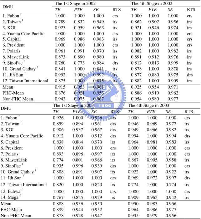
(51) market share.. This fact further confirms that the large-sized SFs are able to capture. larger market shares.. 4.2. The Findings of the Four-Stage DEA 4.2.1. Stage One: Initial DEA (The CCR and BCC Input-Oriented Models). This DEA model includes two outputs and two inputs.. Efficiency scores for. twelve integrated securities firms in 2002 and fourteen integrated securities firms in 2005 are computed using an input orientation and variable returns to scale technology.. Table 4-2 shows the initial result from the stage 1. efficiency (TE) of ISFs is 0.915 in 2002.. The average technical. The mean TE (0.876) of ISFs under FHC is. obviously less than the mean TE (0.943) of ISFs without joining an FHC.. Research. shows that it is not only the efficient Integrated Securities Firms (ISFs) that are allied with banks to form a financial holding company.. Based on the result of technical. efficiency in the first stage, only one of the efficient ISF became an FHC’s subsidiary in 2003.. In addition, the average technical efficiency among ISFs has been. increasing from 0.888 in 2003 to 0.928 in 2005 from the first-stage DEA results.. It. shows that forming an FHC imposes a threat and creates incentives for efficiency score.. One year before most FHCs were established in 2002, 67 percent of the ISFs. in the sample have increasing returns to scale; 25 percent of the ISFs have constant returns to scale.. There is only one ISF with the decreasing returns to scale that is the. subsidiary of an FHC, because this FHC was approaching to merge with another bank and did not dedicate its efforts on the securities business.. During 2003-2004, Fubon. Securities, Taiwan Securities, KGI Securities, and Sinopac Securities have decreasing returns to scale owing to expanding their business via acquiring other specialised securities.. Three-fourths ISFs are under an FHC. 42. Non-FHC ISFs were trying to.