國 立 交 通 大 學
電子工程學系 電子研究所碩士班
碩 士 論 文
適用於 MIMO OFDM 系統之 V-BLAST 偵測技術的研
究與其改善設計
Investigation of V-BLAST Detection Technique and Its
Improvement for MIMO OFDM Systems
研 究 生:張譽桀
指導教授:陳紹基 博士
適用於 MIMO OFDM 系統之 V-BLAST 偵測技術的研
究與其改善設計
Investigation of V-BLAST Detection Technique and Its
Improvement for MIMO OFDM Systems
研 究 生:張譽桀 Student:Yu-Chieh Chang
指導教授:陳紹基 博士 Advisor:Sau-Gee Chen
國 立 交 通 大 學
電子工程學系 電子研究所碩士班
碩 士 論 文
A ThesisSubmitted to Department of Electronics Engineering & Institute of Electronics College of Electrical Engineering and Computer Science
National Chiao Tung University in partial Fulfillment of the Requirements
for the Degree of Master
in
Electronics Engineering
July 2006
適用於 MIMO OFDM 系統之 V-BLAST 偵測技術的研
究與其改善設計
學生:張譽桀 指導教授:陳紹基 博士
國立交通大學
電子工程學系 電子研究所碩士班
摘 要
本論文討論 MIMO-OFDM 訊號偵測的相關技術,特別是 V-BLAST 技
術。還有介紹各種關於 V-BLAST 演算法的變化技術,依效能不同有高
複雜度也有低複雜度,我們提出新的 MIMO-OFDM 訊號偵測演算法首先
簡化最大可能性技術(ML)大量的複雜度並結合此簡化之 ML 技巧和
V-BLAST 以兼顧複雜度與效能表現。經由複雜度比較和位元錯誤率
(BER)效能模擬,結果顯示我們提出的演算法性能比 V-BLAST 好並且
只會增加一小部分的複雜度。
Investigation of V-BLAST Detection Technique and
Its Improvement for MIMO OFDM Systems
Student: Yu-Chieh Chang Advisor: Sau-Gee Chen
Department of Electronics Engineering & Institute of Electronics
National Chiao Tung University
Abstract
In this thesis, signal detection techniques for MIMO OFDM systems are investigated, particularly the V-BLAST technique. In addition, all the enhanced and modified detection methods based on V-BLAST are studied. Those techniques may have higher or lower complexities than V-BLAST technique, depending on their performance. In order to achieve high-performance detection with low complexities we propose a new detection algorithm by combining a simplified maximum likelihood method with V-BLAST detection. Simulation results and complexity comparisons show the proposed methods achieve better performances than the conventional method at the cost of small complexities.
誌謝
在這兩年之中我的指導教授陳紹基博士,對我們的課業研究方向
提供了很多幫助在這兩年中對於我的課業研究著實提供了許多幫助,
除了他扎實的知識,還有遊歷過不少國家的趣聞,都是值得我再三回
味,在此獻上由衷的感激。
此外要感謝的是實驗室 429 的同學們,在課業上提供我不少的幫
助,可以談心說地,並且在生活上互相幫助,在這不短不長的兩年研
究所生涯之中,很高興能夠有金融、昀震、文威、敏杰的陪伴,也祝
福他們在未來的人生之中能夠發揮在這裡學到的東西,並且迎向燦爛
的人生;建全學長也給了我們關於課業還有未來工作上面的建議,讓
我們對未來有更進一步的認知,而不再感到惶恐,在此由衷的感激,
在快要離開交大的這個時刻,希望以後大家能夠固定時間約出來聊聊
近況。
最後,要感謝我的父母,給我很多包容還有經濟上的支柱,使得
我能夠平安順利的完成學業,謝謝。
Contents
中文摘要... Ⅰ ABSTRACT... Ⅱ 誌謝... Ⅲ CONTENTS... Ⅳ LIST OF TABLES ... Ⅵ LIST OF FIGURES ... Ⅶ Chapter 1 Introduction 1 1.1 Background ... 1 1.2 Motivations ... 21.3 Organization of the Thesis ... 3
Chapter 2 OFDM and MIMO Fundamentals 4
2.1 OFDM System Models ... 4
2.1.1 Continuous Time Model ... 5
2.1.2 Discrete Time Model... 7
2.1.3 Effect of Cyclic Prefix ... 8
2.2 Concept of Multiple-Input Multiple-Output (MIMO) Systems... 8
2.2.1 MIMO System Model ... 9
2.2.2 MIMO-OFDM Architecture...11
2.2.3 An example MIMO OFDM System EWC 802.11n ... 12
2.3 Signal Detection Algorithms for MIMO Systems ... 15
2.3.1 Maximum-Likelihood (ML) Detection... 16
2.3.2 V-BLAST Detection Method ... 16
2.3.3 Detection Methods based on V-BLAST ... 18
2.3.3.1 Simplified V-BLAST Detection... 18
2.3.3.2 Enhanced V-BLAST Detection... 20
2.3.3.2.1 Two Iterative V-BLAST Detection Algorithms ... 20
2.3.3.2.2 Enhanced Zero-Forcing V-BLAST Detection... 25
2.3.3.2.3 Joint ML and DFE Scheme for V-BLAST ... 27
2.3.3.3 The MMSE-BLAST Detection Method... 28
2.3.3.3.1 Modified Channel Matrix on the MMSE V-BLAST Technique ... 29
2.3.3.4 V-BLAST Technique with Parallel Symbol Cancellation... 30
2.3.4 Comparisons of Data Detection Algorithms ... 32
Chapter 3 The Proposed Data Detection Algorithms 35 3.1 The New Detection Methods ... 35
3.1.1 New Hybrid ML and V-BLAST Detection Method... 36
3.1.2 Extension of the new method... 38
3.2 The Compared Detection Techniques ... 39
3.3 Reducing Computational Complexities in Pseudo-Inverse ... 40
3.4 Complexity Analysis and Comparison... 41
Chapter 4 Simulation Results 45
4.1 Performance – Execution Time... 46
4.2 Performance – Bit Error Rate ... 49
Chapter 5 Conclusion 64
List of Tables
Table 2.1 Parameters and specifications of EWC 802.11n systems [11] 13 Table 2.2 Change of diversity degree in each V-BLAST’s loop [19] 21 Table 2.3 Number of pseudoinverses of the Li’s and Shen’s approaches [21] 24 Table 2.4 Complexity comparisons of data detection algorithms 33 Table 3.1 Multiplication complexities of various detection algorithms without
considering matrix symmetry 42 Table 3.2 Multiplication complexities of various detection algorithms, considering
matrix symmetry 43
Table 4.1 Simulated EWC system parameters 46 Table 4.2 Multiplication complexities of the proposed detection algorithms vs. L
value, considering matrix symmetry 48 Table 4.3 Indoor channel model [28] with short delays, office environment 49 Table 4.4 Indoor channel model [28], large hallenvironment
56
List of Figures
Figure 2.1 Cyclic prefix of an OFDM symbol [18] 5 Figure 2.2 Spectrum of an OFDM signal [18] 6 Figure 2.3 (a) Continuous-time OFDM baseband modulator [18] 6 Figure 2.3 (b) Continuous-time OFDM baseband demodulator [18] 6 Figure 2.4 Discrete-time OFDM system model [18] 7 Figure 2.5 Wireless MIMO transmission model [17] 10 Figure 2.6 Transmitter architecture of a MIMO OFDM system [10] 11 Figure 2.7 Receiver architecture of a MIMO OFDM system [10] 12 Figure 2.8 PLCP frame format of EWC 802.11n standard [12] 14 Figure 2.9 Cyclical delay format of the preamble in EWC 802.11n standard [11] 15 Figure 2.10 The 0th-order simplified V-BLAST detection algorithm in [13] 18 Figure 2.11 The simplified V-BLAST detection algorithm in [18] 19 Figure 2.12 Li’s iterative V-BLAST detection algorithm 24 Figure 2.13 Equation (2.16) as function of || ||
∩
n [22] 25
Figure 2.14 Equation (2.17) as function of || ||
∩
n [22] 26
Figure 2.15 ML detection equation (number of transmitter antennas =N ) t 27
Figure 2.16 ML detection equation (number of transmitter antennas =p ) 27
Figure 3.1 The proposed hybrid ML and V-BLAST detection 37 Figure 3.2 The proposed hybrid ML and V-BLAST detection (simplest case forL=1)
37 Figure 3.3 Flow diagram of the proposed hybrid ML and V-BLAST detection (the
most complex case,L= Nt) 38
Figure 3.4 Extension of the proposed algorithm 39 Figure 3.5 Simplified Multiplication Complexities of HHH 41 Figure 4.1 Computation time comparision of the existing detection methods and the
proposed methods (Nt =4 Nr =4) 47
Figure 4.2 Computation time comparision of the existing detection methods and the
proposed methods (Nt =4 Nt =5) 47
Figure 4.3 Computation time comparision of the existing detection methods and the
proposed methods (Nt =4 Nr =6) 48
Figure 4.4 BER performance versus SNR of various detection techniques (2x2), office
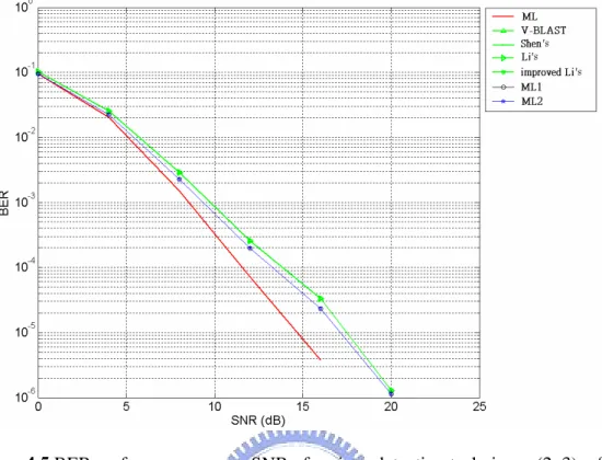
environment 50 Figure 4.5 BER performance versus SNR of various detection techniques (2x3), office
environment 51 Figure 4.6 BER performance versus SNR of various detection techniques (2x4), office
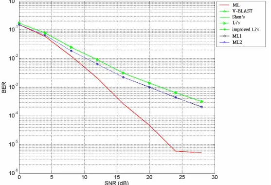
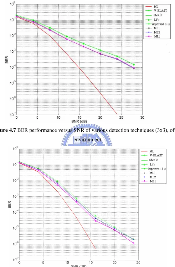
Figure 4.7 BER performance versus SNR of various detection techniques (3x3), office
environment 52 Figure 4.8 BER performance versus SNR of various detection techniques (3x4), office
environment 52 Figure 4.9 BER performance versus SNR of various detection techniques (3x5), office
environment 53 Figure 4.10 BER performance versus SNR of various detection techniques (4x4),
office environment 53 Figure 4.11 BER performance versus SNR of various detection techniques (4x5),
office environment 54 Figure 4.12 BER performance versus SNR of various detection techniques (4x6),
office environment 54 Figure 4.13 BER performance versus SNR of our various detection techniques and
V-BLAST (4x4), office environment 55 Figure 4.14 BER performance versus SNR of our various detection techniques and
V-BLAST (4x5), office environment 55 Figure 4.15 BER performance versus SNR of the proposed detection techniques and
V-BLAST (4x6), office environment 56 Figure 4.16 BER performance versus SNR of various detection techniques (2x2),
large hall environment 57 Figure 4.17 BER performance versus SNR of various detection techniques (2x3),
large hall environment 57 Figure 4.18 BER performance versus SNR of various detection techniques (2x4),
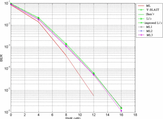
large hall environment 58 Figure 4.19 BER performance versus SNR of various detection techniques (3x3),
large hall environment 58 Figure 4.20 BER performance versus SNR of various detection techniques (3x4),
large hall environment 59 Figure 4.21 BER performance versus SNR of various detection techniques (3x5),
large hall environment 59 Figure 4.22 BER performance versus SNR of various detection techniques (4x4),
large hall environment 60 Figure 4.23 BER performance versus SNR of various detection techniques (4x5),
large hall environment 60 Figure 4.24 BER performance versus SNR of various detection techniques (4x6),
large hall environment 61 Figure 4.25 BER performance versus SNR of our various detection techniques and
Figure 4.26 BER performance versus SNR of our various detection techniques and V-BLAST (4x5), large hall environment 62 Figure 4.27 BER performance versus SNR of our various detection techniques and
Chapter 1
Introduction
1.1 Background
The fast growth of telecommunication service subscribers, the Internet, and the personal computing devices are witnessed in the recent decade and expected to continuous in the future. For wireless multimedia and data services we need robust, high-bit-rate and wide-area wireless networks. Hence, future wireless personal communication systems are expected to provide high performance transmission over hostile mobile environments regardless of mobility or location, although there are still technical problems to be solved for this objective [l]. When realizing broadband wireless systems, those severe effects of frequency-selective fading are difficult to resolve [2]. Traditionally, more bandwidth is required for higher data-rate transmission. However it is often impractical or sometimes very expensive to increase bandwidth. OFDM technique get lot of attraction in wireless transmission in recent years for advantages in mitigating the detrimental effects of frequency-selective fading [3,4,5].
Recent information theory on multiple input multiple output (MIMO) technology reveals that multipath wireless channels facilitate increase of spectral efficiency, provided that those multipath are sufficiently rich [6,7,8]. In such cases, the channel between each transmit and receive antenna pair is flat and uncorrelated. Space Division Multiplexing
(SDM) is a technique that can provide a significant improvement in capacity and bit error rate (BER) performance. Basically, different parallel data streams are transmitted, at the same time and on the same frequency, using an antenna array. When utilizing multiple antennas at the receiver as well, these data streams, mixed-up by the wireless channel, can be recovered by SDM techniques such as Vertical – Bell Laboratories Layered Space-Time (V-BLAST) [9] .
These algorithms require flat-fading channel information between each transmit and receive antenna pair. However, most practical channels are frequency-selective fading so that performances will be degraded. In OFDM systems frequency-selective fading become flat-fading in each subcarrier and is effective when combined with SDM techniques [10, 13].
Currently, plenty of researches are about applying transmitter and receiver diversity [14, 15] and space-time codes [16] to multicarrier techniques. The difference between the combined technique and the previous mentioned combined SDM and OFDM technique is that the latter can improve SNR performances as well as data rates, because it transmits simultaneously different data in different transmit antennas.
1.2 Motivations
In this thesis, we focus on telecommunication systems with rich scattering channels where SDM techniques have best performance. In addition, OFDM systems are studied, because it helps to turn the frequency-selective fading into flat-fading conditions. It is known that for each OFDM subcarrier, transmitted signals experience flat-fading channels. It conforms to the assumed conditions when using ZF and V-BLAST techniques.
In order to get better performance than V-BLAST, we propose a hybrid ML detection and V-BLAST detection, and reduce a good deal of complexities required by ML detection. To get knowledge on computational complexities and BER performances of the proposed algorithms, 802.11n systems with MIMO conditions are simulated. To
verify performances, we analyze and simulate, the proposed designs and some existing designs, with respect to BER and complexity.
1.3 Organization of the Thesis
First, fundamentals of both OFDM and MIMO are studied in Chapter 2, and so are the techniques based on V-BLAST data detection. Besides, MIMO OFDM systems are also described in Chapter 2, followed by discussion of some existing enhanced algorithms for data detection. Chapter 3 introduces the proposed new enhanced MIMO OFDM data detection algorithms based on some major existing algorithms and the devised new idea, while Chapter 4 includes simulations. Simulations are performed according to EWC 802.11n specifications. Finally, we conclude with some remarks of the work in Chapter 5.
Chapter 2
OFDM and MIMO Fundamentals
2.1 OFDM System Models
The principle of multicarrier system is to seperate the data stream into several parallel ones, each modulated by a specific subcarrier and discrete Fourier Transform (DFT) is used in the baseband modulation and demodulation. Through this approach, only a pair of oscillator (for I-part and Q-part) is needed instead of multiple oscillators to modulate different signals at different carriers.
When signals pass through a time-dispersive channel, inter-symbol interference (ISI) and inter-carrier interference (ICI) usually occur in the receiver and cyclic prefix (CP) is introduced to combat ISI and ICI. Cyclic prefix, shown in Figure 2.1, is a copy of the tail part of a symbol, which is inserted in between the symbol to be transmitted and its preceding symbol. As long as the cyclic prefix length is longer than its experiencing time-dispersive channel length, ISI can be avoided. At the same time, the cyclic prefix along with its symbol makes a periodic signal and maintains the properties of circular convolution and subcarrier orthogonality that prevents the ICI effect.
Figure 2.1 Cyclic prefix of an OFDM symbol [18]
2.1.1 Continuous-Time Model
In this chapter, a continuous-time model is used to introduce the whole OFDM baseband system including the transmitter and receiver. In the transmitter, the transmitted data is split into multiple subchannels with overlapping frequency bands.
The spectrum of OFDM signal is shown in Figure 2.2. It is clear that the spectrum of each subchannel is spreading to all the others, but is zero at all the other subcarrier frequencies, because of the sinc function property, which is the key feature of the orthogonality.
Assume the given channel is quasi-static, i.e., constant during the transmission of an OFDM symbol and variable symbol wise, where the quasi-static impulse response is
) , ( mn
h , n is the time index and m is the channel path delay. The received signal ) (t y can be expressed as ) ( ) ( ) , ( ) (t h n m x t nt y = ∗ + (2.1)
where x(t) is the transmitted data and n(t) is the additive white Gaussian noise.
Figure 2.3 (a) shows a typical continuous-time OFDM baseband modulator, in which the transmitted data is split into multiple parallel streams which are modulated by different subcarriers and then transmitted simultaneously. At the receiver, the received signal is demodulated simultaneously by multiple matched filters and then the data on each subchannel is obtained by sampling the outputs of matched filters, as shown in Figure 2.3 (b).
Cyclic prefix
Ts Tg
Figure 2.2 Spectrum of an OFDM signal [18]
Figure 2.3 (a) Continuous-time OFDM baseband modulator [18]
2.1.2 Discrete-Time Model
As mentioned previously, to simultaneously transmit multiple data, the transmitter must modulate data with multiple subcarriers and the receiver must demodulate with multiple matched filters. In fact, the modulation and demodulation can be implemented efficiently by using digital IDFT/DFT operations, because they can be respectively represented as
∑
∑
− = − = = = 1 0 2 1 0 ) ( ) ( ) ( ) ( N k k ki N j N k i k X e k X i x φ π (2.2)∑
∑
− = − − = = = 1 0 2 1 0 ) ( ) ( ) ( ) ( N k k ki N j N k i k y e i y k Y ψ π (2.3) which are the same as IDFT operation of the transmitted data X(k) and DFT operationof the received data y(i), respectively.
Figure 2.4 shows the discrete-time baseband OFDM model. The IDFT transforms the frequency-domain data into time-domain data which is delivered over the air and passed through a multi-path channel, denoted as h( mn, ). At the receiver, to recover the signal in frequency domain, DFT is adopted in the demodulator as a matched filter. Then the frequency-domain signal of each subchannel is obtained from its DFT output.
2.1.3 Effect of Cyclic Prefix
Because of multipath channels, orthogonality as shown in Figure 2.2 will be destroyed by ISI and ICI. However, as long as the cyclic prefix length is longer than that of h( mn, ), ISI effect can be avoided. It is known that circular convolution in time domain results in multiplication in frequency domain when the channel is stationary so that the received signal y(k) in frequency domain is the product of transmitted data x(k) and subcarrier channel response H(k). Thus, the orthogonality is maintained (if h( mn, ) is fixed within the symbol length) and data can be easily recovered by one-tap channel equalizer, i.e., dividing y(k) by the correspondingH(k).
) ( ) ( ) ( ) (k H k x k n k y = × + (2.4)
2.2 Concept of Multiple-Input Multiple-Output (MIMO)
Systems
MIMO system architectures provide better spectral efficiency than conventional systems, because of the benefit of multiple antenna or space diversity both at the transmitter and receiver.
MIMO systems provide the ability to turn multipath propagation, which is traditionally a drawback of wireless transmission, into a benefit. Since MIMO systems effectively take advantage of random fading and multipath delay spread, the signals transmitted from each transmit antenna appear highly uncorrelated at each receive antenna and the signals travel through different spatial channels. Then the receiver can exploit these different spatial channels and separate the signals transmitted from different antennas at the same frequency band simultaneously.
2.2.1 MIMO System Model
MIMO is a promising technology suited for high-speed broadband wireless communications. Through space division multiplexing, MIMO technology can transmit multiple data streams in independent parallel spatial channels, thereby increasing total system transmission rate.
MIMO systems can be easily defined. Considering an arbitrary wireless communication system, a link is considered for which the transmitter is equipped with Nt
transmit antennas and the receiver is equipped with Nr receive antennas. Such a setup is
illustrated in Figure. 2.5. Consider this system some important assumptions are made first: 1. Channels are constant during the transmission of a packet. It means the communication is carried out in packets that are of shorter time-span than the coherence time of the channels.
2. Channels are memoryless. It means that an independent channel realization is drawn for each use of the channels.
3. The channel is flat fading. It means that constant fading over the bandwidth is desired in the case of narrowband transmissions. It also indicates that the channel gains can be represented by complex numbers.
4. The received signal is corrupted by AWGN only.
With these assumptions, it is common to represent the input/output relations of a narrowband, single-user MIMO link by the complex baseband vector notation
n Hx
y= + (2.5)
where x is the Nt×1 transmit vector, y is the Nr×1 receive vector, H is the Nr×Nt channel
matrix, and n is the Nr×1 additive white Gaussian noise (AWGN) vector at some instant
in time. All the coefficients hij comprise the channel matrix H and represent the complex
gain of the channel between the jth transmit antenna and the ith receive antenna. The channel matrix can be written as
⎟ ⎟ ⎟ ⎟ ⎟ ⎠ ⎞ ⎜ ⎜ ⎜ ⎜ ⎜ ⎝ ⎛ = t r r r t t N N N N N N h h h h h h h h h H L M O M M L L 2 1 2 22 21 1 12 11 (2.6)
ij j ij ij ij ij j h e h =α +β = ⋅ φ (2.7)
Coefficients {hij} reflect unknown channnel properties of the medium, usually
Rayleigh distributed in a rich scattering environment without line-of-sight (LOS) path. If
ij
α and βij are independent and Gaussian distributed random variables, then |hij| is a
Rayleigh distributed random variable. Actually, coefficients {hij} are likely to be subject
to varying degrees of fading and change over time. Therefore, determination of the channel matrix is an important and necessary aspect of MIMO techniques. If all these coefficients are known, there will be sufficient information for the receiver to eliminate interference from other transmitters operating at the same frequency band.
Figure 2.5 Wireless MIMO transmission model [17]
Although the introduced MIMO transmission requires flat-fading channels, and it is limited to applications with narrowband transmissions, in real broadband transmission systems, channel conditions are often frequency-selective fading. A technique alleviating severe effect of frequency-selective fading is demanded. OFDM technique is a good solution for this purpose in wireless transmission owing to its advantages [3,4,5].
2.2.2 MIMO-OFDM Architecture
According to Section 2.1, OFDM technique turns frequency-selective fading channel into several flat-fading subchannels, and it solves the major problem in wideband transmission systems. Boubaker et. al [10] proposed V-BLAST technique to detect transmitted signals on each subcarrier of a MIMO OFDM system. MIMO OFDM transceiver and receiver architecturs are shown in Figures 2.6 and 2.7, respectively.
Subchannels are orthogonal to each other in OFDM systems. Hence, in a single-input-single-output (SISO) OFDM systems, the received signals are product of channel response and transmitted signal, as shown in equation 2.4. In MIMO systems, signals transmitted from different antennas on a subcarrier simultaneously interfere each other, but signals at different subcarriers are independent. At each receiver antenna, a linear combination of the transmitted signal and channel response on each subcarrier is observed. That corresponds to assumptions of MIMO systems. On each subchannel, a space division multiplexing (SDM) like V-BLAST is applied. That is, the task is to recover x from the received signal y and channel state information (CSI) H on each subcarrier.
Figure 2.7 Receiver architecture of a MIMO OFDM system [10]
2.2.3 An example MIMO OFDM System EWC 802.11n
EWC 802.11n standard utilize both MIMO and OFDM techniques for high throughput transmission of wireless LAN. EWC 802.11n proposal [11] emphasizes backward compatibility with existing installed base, building on experience with interoperability in 802.11g and previous 802.11 amendments which are mainly designed for indoor wireless internet applications. Hence, we review the physical layer of wireless LAN 802.11a [12] system which is based on OFDM technology. The main system parameters of IEEE 802.11n Wireless LAN standard are listed in Table 2.1.
In 802.11n standard, a frame is composed of three fields. Table 2.1 shows the packet format which facilitates synchronization and channel estimation of the receiver. In the preamble field, the preambles are composed of ten repeated short symbols and two repeated long symbols. The total duration of short symbols is 8µs and so is that of long symbols. Since the SIGNAL field contains the most important information of a packet, such as frame length and modulation, synchronization and channel estimation must be finished before decoding of the SIGNAL field.
To examine validity of proposed algorithms in latter chapters, EWC 802.11n standard, is adopted for simulation.
Table 2.1 Parameters and specifications of EWC 802.11n systems [11]
In 802.11n, a PLCP (PHY Layer Convergence Protocol) frame shall have one of the following three formats, the field parameters are define below:
Figure 2.8 PLCP frame format of EWC 802.11n standard [12]
L-STF: Legacy Short Training Field. L-LTF: Legacy Long Training Field. L-SIG: Legacy Signal Field.
HT-SIG: High Throughput Signal Field.
HT-STF: High Throughput Short Training Field. HT-LTF1: First High Throughput Long Training Field.
HT-LTF’s: Additional High Throughput Long Training Fields. Data: The data field includes the PSDU (PHY Sub-Layer Data Unit). The PHY will operate in one of 3 modes:
-Legacy mode: in this mode the packets are transmitted with 802.11a/g format. -Mixed mode: in this mode packets are transmitted with a preamble compatible with the legacy 802.11a/g – the legacy Short Training Field (STF), the legacy Long Training Field (LTF) and the legacy signal field are transmitted so they can be decoded by legacy 802.11a/g devices. The rest of the packet has a new format. In this mode the receiver shall be able to decode both the Mixed Mode packets and legacy packets.
-Green Field: in this mode high throughput packets are transmitted without a legacy compatible part. This mode is optional. In this mode the receiver shall be able to decode both Green Field mode packets and legacy format packets.
For the purpose of compatibility with 802.11 legacy devices, the legacy part of the preamble format in EWC proposal is the same as that in 802.11a. If the legacy preambles are transmitted from multiple antennas, the mapping of this single spatial stream to multiple antennas has to be done such that beamforming in far-field is mitigated. One method for achieving this is to use a cyclical-delay-diversity (CDD) mapping. The cyclical delay is adopted in EWC proposal, whose format is used for simulation. Figure 2.9 shows the cyclical delay format in EWC. The maximum number of the spatial data streams is four. STRN stands for the short training sequence. LTRN represents the long training symbol. GI2 is the guard interval of the long training symbol.
Figure 2.9 Cyclical delay format of the preamble in EWC 802.11n standard [11]
2.3 Signal Detection Algorithms for MIMO Systems
Signal detection here means a process that try to recover the transmitted signals at receivers. As shown in equation 2.5, the task is to detect the transmitted vector x based on
received vector y and channel state information (CSI) H.
In this section zero-forcing (ZF) criterion is considered due to consideration of low complexity. Zero-forcing techniques receive an input vector y and send it to a filter bank which eliminates the mutual interference without caring about noise.
STRN 400 ns cs STRN STRN 600 ns cs GI21 LTRN GI2 GI23 LTRN 100 ns cs LTRN 1700 ns cs GI22 LTRN 1600 ns cs STRN 200 ns cs
2.3.1 Maximum-Likelihood (ML) Detection
Since modern transmission systems are digital, each element of transmitted vector
x is chosen from a finite set, which is denoted as A, such as BPSK, QPSK and 16-QAM.
Hence, a transmitted signal x belongs to the multiplicative set ANt. The optimum
maximum-likelihood (ML) detector searches over the whole set of transmit signals x ∈ ANt, and decides in favor of the transmit signal xML that minimizes the Euclidian distance
to the receive vector y , i.e.
2 min
arg y Hx
xML = x∈ANt − (2.8)
The computational effort is of order MNt, where M denotes the size of finite set A. When using high modulation scheme or a large number transmitting antennas, ML detection is impractical.
2.3.2 V-BLAST Detection Method
Although ML detection reaches optimal performance, it is not feasible for large numbers of transmit antennas or high modulation schemes. In the sequel, some suboptimal algorithms are investigated. The target is to find algorithms that have performance near ML and low complexities.
Vertical – Bell Laboratories Layered Space-Time (V-BLAST) [9] is proposed to improve performance of the linear detection method by utilizing successive interference cancellation based on zero-forcing criterion. It suggests that transmitted signals are detected sequentially rather than in parallel. In each detection step, the signal which yields the smallest estimation error is linearly detected. It is shown in [9] that row gZF, the
row with the minimum norm in GZF (GZF H HHH HH
1 ) ( − + =
= ), has the largest
signal-to-noise ratio (SNR) and yields the smallest estimation error, because it causes minimum noise enhancement.
(
)
i i i ZF i ZF i g y g Hx n x x = = + = +η ∩ (2.9)i
x
∩
is quantized to obtain estimate of x , and the interference of this signal is i
removed by subtracting it from the received signal y, so is the i -th column of the channel
matrix is nulled. Nulling and canceling process are repeated until all signals are detected, as summarized in the following algorithm steps:
Begin
H
H1 = (2.10.a)
y
y1 = (2.10.b)
for (i=1; i <=Nt; i++) (2.10.c)
( )
+ = i i ZF H G (2.10.d) i ZF i i Gk =arg min (2.10.e)
( )
ki i ZF i ZF G g = (2.10.f) y g x i ZF i = ∩ (2.10.g) ⎟ ⎠ ⎞ ⎜ ⎝ ⎛ = ∩i k quantize x x i (2.10.h) i i k k i i y x H y+1= − (2.10.i) i i i k H H +1= (2.10.j) endwhere (G)i means i -th row of G, H means ki k -th column of H, and i i ki
H means the
resulting H matrix after nulling the k -th column of i i
H .
The main computational bottleneck in the iterative process is the computation of pseudo inverses for Nt matrices. For saving computation, channel response is assumed
constant within a packet, as assumption 1 suggests. The optimal detection order and each nulling vector gZF are validly used to detect received signals in the whole packet,
because they share the same channel matrix. That is, pseudo inverse of the channel is not updated.
2.3.3 Detection Methods based on V-BLAST
We will introduce four different algorithms based on V-BLAST technique. The first algorithm reduces the numbers of pseudo-inverse operations. The second algorithms can increase performance by reducing negative side effects. The first and second algorithms consider trade-off in the iteration process of V-BLAST techniques. The third algorithm is MMSE-VBLAST that includes the noise term in the design of the linear filter matrix G. The fourth algorithm is based on parallel symbol cancellation (PSC)
instead of serial symbol cancellation (SSC). It focuses on detecting signals at the same time.
2.3.3.1 Simplified V-BLAST Detection
On each subcarriers of a MIMO ODFM system, a V-BLAST detector is used, because we can formulate the detection problem of each subchannel by equation 2.5. Hence for practical OFDM systems, there will involve a lot of V-BLAST detectors. Fortunately, channel responses of successive subcarriers are often similar. Some simplified algorithms [13,20] are proposed based on this observation.
[13] assumed that successive subcarriers have the same channel response so that calculated vectors of a subcarrier are applied to detect signals of nearby subcarriers. We can call this algorithm a simplified 0th-order algorithm.
The subcarrier which is decoded by approximation is assumed to have the same decode order as that of the subcarrier which provides the pseudo inverse. At each step of V-BLAST detection, a column of channel matrix is set to zero in order to ignore the effect of the corresponding transmitting antenna. If the pseudo inverse is used to estimate inverse of adjacent subcarriers, the subcarriers have to recognize the nulled columns, which stand for the detected signals. In other words, the optimal decoding order is assumed unchanged.
Under this assumption, there are some opportunities for further simplification. The simplified algorithm has identical performance but with lower complexities. Owing to unchanged decoding order it merely needs a row of the approximated pseudo inverse which represents the transmitted signal to be detected, rather than the whole pseudoinverse, as shown below.
[
H k p] [
j H k p H k p H k p H k p H k p]
j + + + + ≈ + − + +1, ) ( , ) ( , ) ( ( , ) ( 1, )) ( , ) ( (2.11) where []j denotes the j-th row, and p is a small enough positive integer.[
H k p] [
j H k p] [
j H k p H k p H k p H k p]
j + + + + ≈ + − + +1, ) ( , ) ( , ) ( ( , ) ( 1, )) ( , ) ( (2.12) then[
H(k+1,p)+] [
j ≈ H(k,p)+]
j(1+(H(k,p)−H(k+1,p))H(k,p)+) (2.13) As a result, computation complexity is reduced, but performance is not noticeably degraded. This simplified algorithm can be called a 1st-order simplified algorithm. Its algorithm steps are summarized below.Begin
for (i=1 ; i <= subcarrier number ; i+=2) (2.14.a) calculate weight vectors giZF according to equation (2.10) (2.14.b)
if successive subcarriers share a channel respose [13] (2.14.c)
i ZF i ZF g g+1= (2.14.d) else // (2.14.e)
calculate weight vectors gZFi+1 according to equation (2.13) (2.14.f)
end (2.14.g)
end (2.14.k)
2.3.3.2 Enhanced V-BLAST Detection
Since V-BLAST’s performance is worse than ML detection, improved detection methods [19,21,22] based on V-BLAST technique are proposed to get better performance than the conventional V-BLAST technique.
2.3.3.2.1 Two Iterative V-BLAST Detection Algorithms
Shen’s Approach [19]:
An iterative V-BLAST detection algorithm improving the performance over error propagation is proposed [19]. In the algorithm, low-diversity substreams are iteratively decoded by using decisions from high-diversity substreams. As such the performance is greatly improved over the conventional one. Another advantage of this algorithm is that it is practical to make a trade-off between performance and complexity. The steps of the algorithm is listed below. Table 2.2 also illustrates the algorithm.
initialization: Step 1: detect x x xNt ∩ ∩ ∩ ... , 2 1 by V-BLAST
Step 2:
for i=1 to Nt-1
subtract signals from substreams 1 to i (x x xi
∩ ∩ ∩ .... , 2 1 ) as j i j jx H y y ∩ = ∩
∑
− = 1 (2.15)apply the V-BLAST detection to generate xNt−i
∩
end
Table 2.2 Change of diversity degree in each V-BLAST’s loop [19]
No. of Loop Detection order Detected Symbol
Initialization Loop 1 Loop 2 : : : : Loop Nt Li’s Approach [21]:
In this approach proposed iterative method [21] to suppress error propagation and improve the performance in an uncoded case. From simulation results, this method exhibits considerable performance gains over the original V-BLAST detection algorithm and the iterative algorithm presented in [19]. At the same time, this method has a lower complexity compared with the iterative method in [19].
t N x x x ∩ ∩ ∩ → → 2... 1 1 2 1 .... − ∩ ∩ ∩ ∩ → → t T N N x x x x 2 2 1 1 ... , − ∩ ∩ ∩ − ∩ ∩ → → t t t N N N x x x x x 1 2 1...., , ∩ ∩ − ∩ ∩ → x x x xNt Nt t N x ∩ 1 − ∩ t N x 2 − ∩ t N x 1 ∩ x
Since the detected symbol xNt
∩
has a diversity order of Nr, the new-version
symbols of new Nt x x1.... −1 ∩ ∩
are more accurate than the old version. Such an improvement is especially obvious for symbol 1
∩
x , because the new-version 1
∩
x has the diversity order of
Nr while the old one only has the diversity order of 1. By using such an approach,
closed-loop iteration architecture for V-BLAST detector can be constructed. In detail, if the new-version 1
∩
x is different from the old one, repeat above procedure. Otherwise,
terminate the procedure and the symbol of xNt
∩
as well as the present new-version
new N new t x x1 .... −1 ∩ ∩
will be the final output of the detector. The method’s steps are summarized below. −1−
~
i
H means the resulting H matrix after nulling the i-1th column of H.
Step 1:
Initialize the iteration number as IterNum=0. Step 2:
Perform the optimal ordering and SIC using V-BLAST method and get the
detected symbols Nt old old x x x ∩ ∩ ∩ .... , 2
1 (the optimal order is assumed to be
1,2,….Nt) Step 3: H H = ~ y y= ~ ; t Nt new N x x ∩ ∩ = for i=Nt −1 to 1 new N i x t H y y 1 1 ~ ~ ~ − ∩ −⋅ − = ; 1 ~ ~ − − =Hi H ~ ~ ) (H y xi = i⋅ + ∩ ) ( i i Q x x ∩ ∩ = end
; 1 + = IterNum IterNum Step 4: If IterNum=MaxIterNumOR old new x x1 1 ∩ ∩ = goto step 5; Else new old x x1 1 ∩ ∩ = goto step 4; End Step 5: H H = ~ ; ~ y y= for i= Nt −2 downto 1 old i i x H y y 1 1 ~ ~ ~ − ∩ +⋅ − = ; 1 ~ ~ − + =Hi H ~ ~ ) (H y xi = i⋅ + ∩ ) ( i old x Q xi ∩ ∩ = End ; 0 0 old x x ∩ ∩ = goto step 2 Step 6:
End of iteration and the final detected symbols are
new N new t x x x ∩ ∩ ∩ ... , 2 1
Figure 2.12 Li’s iterative V-BLAST detection algorithm [21]
Assumed that x1....xNnewt−1 are detected in two iterations, shen’s approach requires
more pseudoinverses than those of the Shen’s approach. But their performances are the same [21]. Therefore, we will compare the second approach with the proposed methods in the latter chapters.
Table 2.3 Number of pseudoinverses of the Li’s and Shen’s approaches [21]
Algorithms No. pseudoinverses Original V-BLAST t N Shen’s approach 2 ) 1 ( t+ t N N Li’s approach 2Nt −1
2.3.3.2.2 Enhanced Zero-Forcing V-BLAST Detection
In their article [22], the authors concentrate on ZF decoding in V-BLAST technique and show that the ordering design in the algorithm has some negative side effects. Those effects reduce algorithm’s performance. An improved ordering scheme is then proposed for ZF V-BLAST decoding.
Figure 2.11 [22] demonstrates the behavior of equation ( 2
|| ||ni
∩
) with a solid curve and the lower/upper bounds of
2 2 2 ||) || ( || || ||) || (d ni yi ni d ni ∩ ∩ ∩ + ≤ − ≤ − (2.16) (when d = 2 , ≤ ni ≤d ∩ || ||
0 ) in dotted lines. Divide equation (2.16) by ni +K
∩ 2 || || , one can get K n n d K n n y K n n d i i i i i i i + + ≤ + − ≤ + − ∩ ∩ ∩ ∩ ∩ ∩ 2 2 2 2 2 2 || || ||) || ( || || || || || || ||) || ( (2.17)
Figure 2.13 plot of equation (2.16) vs. || || ∩
Figure 2.14 plot of equation (2.17) vs. || || ∩
n [22]
Conventionally, ki is chosen by equation ( arg min || i ||
ZF i
i G
k = ). Different K will
make different sizes of overlap regions. The smallest overlap region can be obtained in the figure. Therefore, better performance will be obtained by choosing the smallest overlap region. The overlapping region starts to occur when ||ni||
∩
is relatively large. One can normalize the cost function by factor ni +K
∩ 2 || || . Therefore ki is obtained by K n G k i i ZF i i + = 2 ^ || || || || min arg (2.18)
Simulation results [22] show that the new ranking will get better performance than conventional V-BLAST technique.
2.3.3.2.3 Joint ML and DFE Scheme for V-BLAST
In this approach [23], the authors present a detection algorithm, which combines ML and DFE schemes for V-BLAST method. It can improve V-BLAST method’s performance by employing ML detection after V-BLAST detection. It makes a trade-off between complexity and performance, and shows that its performance is better than V-BLAST detection. 2 1 1 1 1 1 11 2 1 || || min arg ⎥ ⎥ ⎥ ⎥ ⎥ ⎥ ⎦ ⎤ ⎢ ⎢ ⎢ ⎢ ⎢ ⎢ ⎣ ⎡ • • ⎥ ⎥ ⎥ ⎥ ⎥ ⎥ ⎥ ⎥ ⎦ ⎤ ⎢ ⎢ ⎢ ⎢ ⎢ ⎢ ⎢ ⎢ ⎣ ⎡ • • • • • • • • • • • − ⎥ ⎥ ⎥ ⎥ ⎥ ⎥ ⎥ ⎥ ⎦ ⎤ ⎢ ⎢ ⎢ ⎢ ⎢ ⎢ ⎢ ⎢ ⎣ ⎡ • • = ∈ t t r r r t r t N N p N N p N N pp p N p N p A x ML x x x h h h h h h h h y y y y x
Figure 2.15 ML detection equation (number of transmitter antennas =N ) t
|| || min arg 1 1 1 11 2 1 ⎥ ⎥ ⎥ ⎥ ⎥ ⎥ ⎦ ⎤ ⎢ ⎢ ⎢ ⎢ ⎢ ⎢ ⎣ ⎡ • • • ⎥ ⎥ ⎥ ⎥ ⎥ ⎥ ⎥ ⎥ ⎦ ⎤ ⎢ ⎢ ⎢ ⎢ ⎢ ⎢ ⎢ ⎢ ⎣ ⎡ • • • • • • • − ⎥ ⎥ ⎥ ⎥ ⎥ ⎥ ⎥ ⎥ ⎦ ⎤ ⎢ ⎢ ⎢ ⎢ ⎢ ⎢ ⎢ ⎢ ⎣ ⎡ • • • = ∈ p pp p p p A x ML x x h h h h y y y x Nt
Figure 2.16 ML detection equation (number of transmitter antennas = p )
This algorithm steps and notations can be illustrated as follows:
Notation: p x x x ∩ ∩ ∩ .... . 2
1 : the estimated values.
Θ : finite set, such as BPSK, QPSK, and 16-QAM ] ... 2 . 1 [ p
] ... .
[x1 x2 xp : the transmitted symbols.
] ... 2 . 1 [ p
H : the channel matrix’s 1~ p columns.
Step 1:
adopt ZF V-BLAST method to get initial decision values. Step 2:
adopt the ML method for the first 1~p subchannels, based on the cost function | ] .. [ | min arg } ... , { [1,2... ] [1,2... ] 1 ... , 2 1 2 1 p p p x x x p y H x x x x x p − = Θ ∈ ∩ ∩ ∩ ∩ ∩ ∩ (2.19) Step 3:
combine the outputs of step 1 and step 2. Step 4:
adopt ZF V-BLAST method to modify the output of step 3.
This algorithm reduces the ML detection in Figure 2.15 to Figure 2.16. But p is hard to choose from design equation [23]. However, in most case one will not use too many receiver antennas. Hence this approach is feasible. This approach must combine V-BLAST technique and ML detection with modification. Still, it is not clear about the modification. However, this approach gives us some thought about hybrid ML detection and V-BLAST detection in Chapter 3.
2.3.3.3 The MMSE-BLAST Detection Method
The way to improve detection performance especially for mid-range SNR values is to replace the ZF nulling operations proposed in [24] with the more effective minimum mean-square error (MMSE) algorithms as shown by equation (2.20).
H n H
ZF H H H
2.3.3.3.1 Modified Channel Matrix on the Performance of MMSE
V-BLAST Technique
In [25], the authors propose a MMSE detection algorithm that exterminates mutual interferences. Hence BER performance is improved. The detection is done by changing the channel matrix after each detection step. The authors also verify the analysis after simulations. Through equation substitution we will compare the mentioned three methods including ZF method, MMSE method [24], and the modified MMSE [25].
In ZF criterion, at the ki-th detection stage because of the orthogonal property
between i k G) ( and i k H)
( , we have the following result
n G x n G Hx G n Hx G y G i i i i i k k k k k ( ) ( ) ( ) ( ) ( ) ) ( = + = + =α + (2.21) where α=[0,0,….,1,…0], whose elements are all zero except the ki-th position. On the
contrary, in the MMSE nulling operation it is not complete zero, and α is given by ] ,... ,.., ,... , [ 2 1 k ki kj kNt k α α α α α α = , where ≠0 i k α (2.22)
The idea here is to reduce interference before the ki sub-stream. The ki-1-th
element of
i
k
G)
( is also zero. As a result, the product vector α is found to be ] ,... ,.., , 0 ,... 0 , 0 [ t N j i k k k α α α α = (2.23)
In conclusion, the interference from the detected sub-stream is suppressed. The method can be summarized as follows.
H H1 = y y1 = 1 ← i k
for (i=1; i <=Nt; i++)
H n n H H I H H G t 1 2 ) ( + − = α G ki =argimin
y G x i i k k =( ) ∩ ⎟ ⎠ ⎞ ⎜ ⎝ ⎛ = ∩ i i k k quantize x x i i k k H x y y= − ( ) 0 ) (H ki = i i k k+1← end
2.3.3.4 V-BLAST Technique with Parallel Symbol Cancellation
Golden's detection process [9] uses techniques of linear-combination nulling and successive symbol cancellation. Like conventional successive symbol cancellation (SSC), Golden's detection algorithm has long time delay. Moreover, the larger the number of transmit antennas, the longer detection delay. Aiming at this problem, a detection algorithm based on parallel symbol cancellation (PSC) is proposed in [26].
2.3.3.4.1 Two-Stage V-BLAST Detection Algorithm
In order to avoid long time delay, parallel symbol cancellation (PSC) was proposed [26]. However the performance will be degraded. To reduce the problem, this two-stage algorithm combines SSC with PSC techniques so as to improve the BER performance. The proposed scheme is combined with ZF technique. The algorithm is divided into two distinct stages.
Stage1: use V-BLAST method to obtain a good initial decision.
Stage2: use parallel symbol cancellation to attain the estimated value of the transmitted vector.
Stage 1:initialization 1 = i + = H G1 2 1 1 argmin||( )j || j G k =
for (i=1; i <=Nt; i++)
i k i k G y x i i,0 =( ) ) ( ,0 0 , ^ i i k k Q x x = i k i i y x H y 1 i,0( ) ∩ + = − 0 ) ( = i k H + + = ki i H G) 1 ( 2 1 ) ... ( 1 argmin||( ) || 1 j i k k j i G k j + ∉ + = end
Stage 2:initialization
for (k=1; k <=Nt; k++) 1 = k 0 , ^ 0 , ^ i k n x x = (n=1,2,3....nt)
∑
≠ = − − = nt n i i i k i k n y x H y , 1 1 , ^ , ( ) (n=1,2,3....nt) (2.24) k n n k n G y x , =( ) , ) ( , , ^ k n k n Q x x = + =[( ) ] ) (G n H n endEquation (2.24) can obtain a diversity order equals the receiver antennas. We will compare this method with the proposed algorithm in Chapter 3.
2.3.4 Complexity Comparisons of Data Detection Algorithms
The 0th-order simplified detection denotes the approach of copied vectors in Section 2.3.3.1. The 1st-order simplified Detection (approximation) denotes is mentioned in section 2.3.3.1. Shen’s and Li’s iterative methods [19] are discussed in Section 2.3.3.2.1. Akhtar’s method [22] denotes the new K approach in Section 2.3.3.2.2, Baro’s method [23] denotes joint ML and DFE scheme in Section 2.3.3.2.3, Duong’s method [25] denotes the approach with modified channel matrix in Section 2.3.3.3.1, while Xiaofeng’s method [26] denotes the PSC method in Section 2.3.3.4.1.
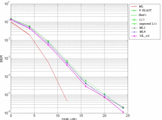
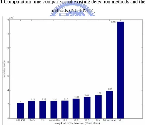
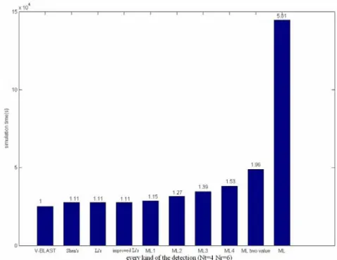
Although complexity of the 0th-order simplified detection method is smaller than the others, it only saves 20% simulation time. For Shen’s and Li’s iterative methods, their performances are similar. However the Li’s iterative method can get more diversity order. Baro’s method is complicated, because it must do V-BLAST detection and ML detection. Moreover, it must computep , which is hard to solve. That is not feasible.
Xiaofeng’s PSC method must detect signal at the same time, so it need many parallel ZF and PSC units [28].
Table 2.4 Complexity comparisons of data detection algorithms No. Multiplication Nt =4,Nr =4 QPSK(A=4) V-BLAST 4 +2 3 + 2 +( 2+ )×6 r t t r t r t t N N N N N N N N 1024 ML N r( t +1) N N A t 5120 Simplified Detection (0th-order appr.) 6 ) (Nt2 +NtNr × 192 Simplified Detection (1st-order appr.) 6 ) ( 2Nt2Nr + Nt2 +NtNr × 320 Shen’s iterative method [19] + × + + + +2 3 2 ( 2 ) 6 4 r t t r t r t t N N N N N N N N 6 ) 1 2 )( 1 ( 2 ) 1 ( + + + + t t t t r tN N N N N N 1094 Li’s iterative method [21] + + + + + t r t r t t r t N N N N N N N N4 2 3 2 ( 2 6 ) ) 1 ( ) 1 (Nt − 2+ Nt− Nr × 1150 Akhtar’s changing k method [22] 6 ) ( 12 2 3 2 2 2 4 + + + + + × r t t t r t r t t N N N N N N N N N 1216 Baro’s joint ML and DFE method [23] + × + + + +2 3 2 ( 2 ) 6 4 r t t r t r t t N N N N N N N N ) 1 ( p + p p N N A
( p is chosen from [8].)
768+ ) 1 ( p + p p N N A Duong’s modified H method [24] 6 ) ( 2 3 2 2 4 + + + + × r t t r t r t t N N N N N N N N 1024 Xiaofeng’s PSC method [25] + × + + + +2 3 2 ( 2 ) 6 4 r t t r t r t t N N N N N N N N 6 ) 3 ( Nt2+NtNr × 1408Chapter 3
The Proposed Data Detection
Algorithms
Since the performance gap between V-BLAST detection and ML detection is significant, we still have a lot of room to improve the V-BLAST techniques. Through technique survey we got some idea from the algorithms in Chapter 2. We will propose a hybrid ML detection and V-BLAST detection method in this chapter. The method will reduce a great deal of the comparison operations in ML detection. It will get better performance than V-BLAST method, without increasing too many comparison operations. Besides, it will decrease complex multiplication in calculating pseudo-inverses.
3.1 The New Detection Methods
As we know joint ML and V-BLAST can get better performance, it provides an idea for further improvement. Specifically, after the initial values x1 to x are detected, Nt
we can use further other detection method like ML detection to do the detection again. First, let us suppose N transmitter antennas and t Nr receiver antennas. If we use
comparisons will have to be made. Generally, in detecting M-QAM by using ML method, a total of (N )t M comparisons need to be made.
We suppose that some of signals are already known. As such, in this way we don’t need to do all the comparisons and it will decrease a large number of comparison operations in ML detection, while still maintain good performances.
3.1.1 New Hybrid ML and V-BLAST Detection Method
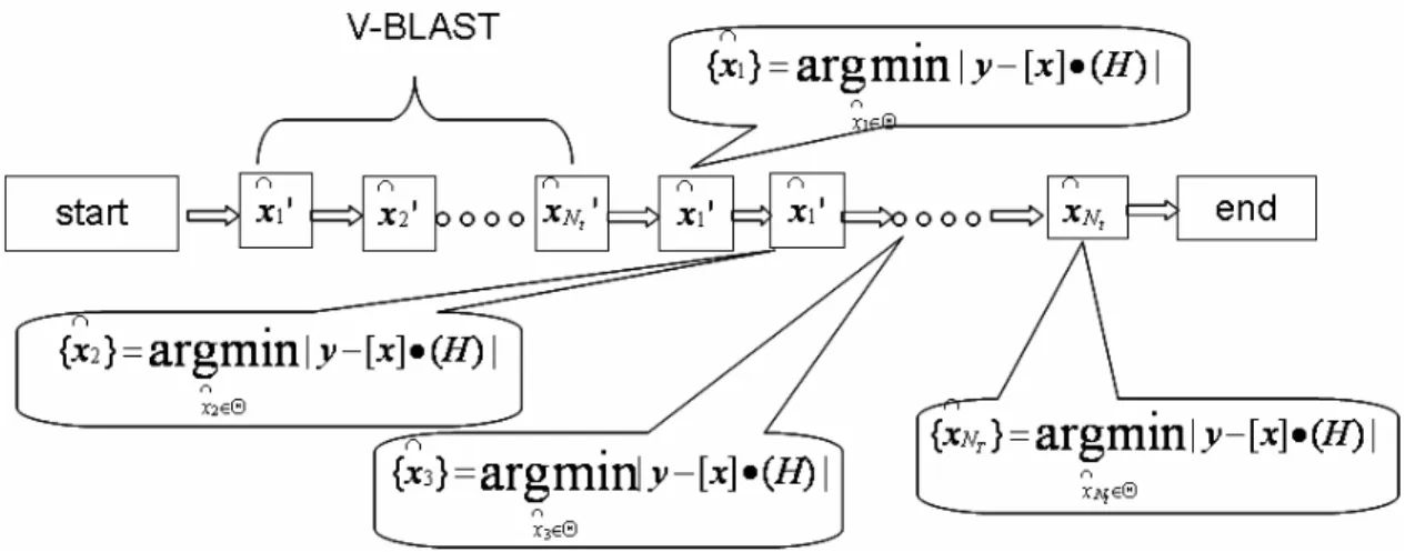
As mentioned before, one can reduce the complexity of equation (2.8), if we already know some detected signals. For example if in M-PSK modulation there is only one unknown symbol, then we just only need to compare M values in ML detection. Based on the idea, first V-BLAST method is used to detect all the initial values, and then we update it by ML detection. Suppose L is the level we want to do the detection, ranging from 1 to N . In other word, we will update L value by ML detection. t
The algorithm is summarized below and shown in Figure 3.1:
Step 1:
adopt V-BLAST method to get the initial x1'...xNT' ∩ ∩
values Step 2:
Based on the known x1'...xNt' ∩ ∩ values, update x xL ∩ ∩ '... 1 values by ML
detection {x } argmin|y [x] (H)|
L x L = − • Θ ∈ ∩
∩ , and the other values (i.e.
T N x xL ∩ + ∩ '... 1 ) by V-BLAST detection
Figure 3.1 The proposed hybrid ML and V-BLAST detection For illustration, we show the detection flow for L=1 and L=Nt in Figure 3.2 and
Figure 3.3, respectively.
Figure 3.3 Flow diagram of the proposed hybrid ML and V-BLAST detection (the most complex case, L=Nt)
In this approach we can confine error propagation, meantime reduce computation complexity. For ML detection, the number of minimum norm we calculate ranging from
M t
N )
( to L×Nt (Θ is M-QAM). We will discuss complexity of the proposed design in Section 3.4 and verify its in Chapter 4.
3.1.2 Extension of the new method
When a system has a large number of transmitter antennas, we can use this approach to detect two or more values at the same time. But here we only discuss the case of detecting two values at the same time. Figure 3.4 depicts the algorithm flow as shown below. The algorithm is summarized below:
Step1:
adopt V-BLAST to get the initial 1'... '
T N x x ∩ ∩ values Step2:
with the detected x1'...xNt' ∩ ∩
values in Step1, update 1', 2' ∩ ∩
x
x by ML
detection based on { , } argmin| [ ] ( )|
1 1, 2 1 x y x H x x x • − = Θ ∈ ∩ ∩ ∩
∩ also update the
other values { 3, 4} ∩ ∩ x x ,{ 5, 6} ∩ ∩ x x ....{xNt1,xNt} ∩ ∩
− using similar method
Figure 3.4 Extension of the proposed algorithm
Although the proposed extended method can get better performance than the proposed method in section 3.1.1, will increase complexity. The complexity will be discussed in section 3.4.
3.2 The Compared Detection Techniques
Li’s and Shen’s methods [19,21]
In 2.3.3.2.1 we introduce these two iterative detection methods, which have similar performances and complexities. In Chapter 4 we will compare Li’s and Shen’s methods in simulation.
Our Improved Li’s method
Shen’s method focuses on optimizing diversity order. It increases diversity order in second loop to get better performance than V-BLAST method. Here, we can modify the Li’s method and increase its diversity order. Precisely equation (3.2) will be used to increase diversity order in the second loop. Therefore, in second loop all the signals will have N diversity orders. The algorithm steps are shown below. (t
− −1 ~ i H means the resulting ~
H matrix after nulling the i-1th column of
~
H ) Step 1:
Perform the optimal ordering and SIC according to V-BLAST method
and get the detected symbols Nt
old old x x x ∩ ∩ ∩ .... , 2
1 (the optimal order is
assumed to be 1,2,….Nt. Step 2: H H= ~ ; ~ y y= t Nt new N x x ∩ ∩ = for i=Nt −1 to 1
∑
≠ = − ∩ = − = nt n i i t i iH n n x y y , 1 1 ~ ~ ~ ) .... 3 , 2 , 1 ( (3.2) ; 1 ~ ~ − − =Hi H ~ ~ ) (H y xi = i⋅ + ∩ ) ( i i Q x x ∩ ∩ = End3.3 Reducing Computational Complexities in Pseudo-Inverse
If H is a m× matrix, then n H H H H H H HH H H H H ) =( ) = ( , and HHH is Hermitian [27]. We can simply compute the elements above diagonal and those below
diagonal are their complex conjugate. In this way we can save some multiplication and addition complexities.
Suppose the thansmitter has N antennas and receiver has t Nr antennas, then
H
HH is Nt byN . Normally, the required number of multiplication operation t HHH
is (Nt)3 . However, considering the mentioned symmetry one can save
2 ) 1 ( ) 1 ( ) ( ) 1 ( ) 1 1 ( 2 2× − = − = − × − + t t t t t t t N N N N N N
N multiplication operations. The
complexity reduction ratio is
t t t t t N N N N N 2 ) 1 ( ) ( 2 ) 1 ( 3 2 − = − . If Nt =4, the ratio is 8 3 , and if 6 = t N the ratio is 12 5
. The simplification skill is used in the simulations of Chapter 4.
Figure 3.5 Hermitian symmetry of matrix HHH
3.4 Complexity Analysis and Comparison
In this section, we will compare the multiplication complexities of the proposed technique with those of V-BLAST detection, ML detection, and the two methods in section 3.2. Table 3.1 shows the approximate multiplication complexities which roughly
fit the simulation time complexities as will be shown in Chapter 4. Multiplication complexities of various detection algorithms for V-BLAST’s channel inversion are
r t r t t N N N N N4 3 2 2 +
From Table 3.1 we know that the ML detection is roughly six-times complicated than that of V-BLAST method. The complexity of the proposed method (L=1) is similar to V-BLAST. But its performance is better than V-BLAST method. Chapter 4 will verify the performances. Table 3.2 considers the matrix symmetry.
Table 3.1 Multiplication complexities of various detection algorithms without
considering matrix symmetry
No of Multiplications Nt=4,Nr=4 (or 5,6) QPSK(A=4) V-BLAST 4 +2 3 + 2 +( 2 + )×6 r t t r t r t t N N N N N N N N 1024 ML ( +1) t r N N N A t 5120 Shen’s method 2 ) 1 ( 6 ) ( 2 3 2 2 4 + + + + × + t r t+ r t t r t r t t N N N N N N N N N N N 6 ) 1 2 )( 1 ( + + +Nt Nt Nt 1094 Li’s method 4+2 3 + 2 +( 2+ +( −1)2 +( −1) )×6 r t t r t t r t r t t N N N N N N N N N N N 1150 Our Improved Li’s method + − + + + + + 3 2 2 2 4 ) 1 ( 2 ( 2 t r t r t t r t t N N N N N NN N N 6 ) ) 1 (Nt− Nr × 1204 Proposed method (L=1) 6 ) ) 1 ( ) 1 ( ( 2 3 2 2 2 4+ + + + + − + − × r t t r t t r t r t t N N N N N N N N N N N ) 1 ( + +ANr Nt 1230 Proposed method (L=Nt) ) 1 ( 4 6 ) ( 2 3 2 2 4 + + + + × + + t r r t t r t r t t N N N N N N N AN N N 1344 Proposed extended method (two values at a time) ) 1 ( 2 6 ) ( 2 3 2 2 2 4 + + + + × + + t r r t t r t r t t N N N N N N N A N N N 1664
![Figure 2.9 Cyclical delay format of the preamble in EWC 802.11n standard [11]](https://thumb-ap.123doks.com/thumbv2/9libinfo/8742469.204436/27.892.215.683.469.700/figure-cyclical-delay-format-preamble-ewc-n-standard.webp)
![Table 4.3 Indoor channel model [28] with short delays, office environment Tap No. Delay (ns) Power (dB) Amplitude Distribution Doppler Spectrum 1 0 0 Rayleigh Classical/Flat 2 36 -5 Rayleigh Classical/Flat 3 84 -13 Rayleigh Classical/Flat 4](https://thumb-ap.123doks.com/thumbv2/9libinfo/8742469.204436/61.892.147.744.461.804/environment-amplitude-distribution-classical-rayleigh-classical-rayleigh-classical.webp)