A novel method for discrete fractional Fourier transform computation

(1)

A NOVEL METHOD FOR DISCRETE FRACTIONAL FOURIER TRANSFORM

COMPUTATION

Soo-Chang Pea

Department of Electrical Engineering, National Taiwan University,

Taipei, Taiwan, R. 0. C.

A B S T R A C T

A novel method for the discrete fractional Fourier transform (DFRFT) computation is given in this paper. With the help of this novel method, the DFRFT of any angle can be computed by the weighted summation of the DFRFTs with the special angles. Moreover, the proposed algorithm is suitable for chirp signal detection and the VLSI implementations.

1. I N T R O D U C T I O N

Fractional Fourier transform (FRFT) is a generalization of Fourier transform, and it indicates a rotation of signal in the time-frequency plane[l). The FRFT has been widely successfully used in the many areas[l][2]. Because of the importance of FRFT, discrete fractional Fourier transform (DFRFT) becomes an important issue in recent years[3][4] [5][6]. In the development of DFRFT, the DFRFT has been considered as the combination of four parts[3]: the origi- nal signal, its DFT, circular flipped of signal and circular flipped of its DFT. This method can be realized by the DFT fast computation aJgorithm[7], but it can not have the similar results as continuous case. In 1996, we have found that the DFRFT with DFT Hermite eigenvectors can have similar outputs as those of the continuous case[5][6]. These DFRFTs use the DFT Hermite eigenvectors as their eigenvectors and have similar eigen decomposition form as continuous FRFT kernel. They can perform a rotation of discrete signals in the time-frequency plane, and have the mixed time and frequency characteristics of discrete signals. The eigen decomposition method have been proved and jus- tified in [SI, and it is successfully used in many applications. The DFRFT discussed in this paper is for the eigen decomposition method[5][6]. Although the eigen decomposition method can have similar results as continuous case, its computation cost is very large. The goal of this paper is to introduce a novel computation method for the DFRFTs

2. R E V I E W O F D F R F T 2.1. Definition of DFRFT

In [5][6][8], the eigen decomposition of the N-point DFRFT is written as the following[5][6]:

F? = V D ? V T (1)

Min-Hung Yeh

Department of Electronic Engineering, National I-LAN Institute of Technology,

Ilan, Taiwan, R. 0. C.

where a indicates the rotation angle of DFRFT. V = [ v o l v l

I

for N is even, V k is the Ic-th order DFT Hermite eigenvector. D? is a diagonal matrix with eigenvalues of DFRFT in the diagonal entries. The methods for finding the DFT Hermite eigenvectors V k are presented in [5][6]. Similar to the eigen decomposition form of continuous FRFT, the k-th order DFT Hermite eigenvector corresponds to the eigenvalue e - J k o . Table 1 shows the eigenvalues of DFRFT. It has been shown in [5][6] that the eigenvalues assignment rule in Table 1 can make the DFRFT be an identity matrix for a = 0 and a DFT kernel matrix for a = ;[5][6]. In Table 1 there exists a jump in the last eigenvalues for the two even cases. So there are some differences in computing the DFRFT kernels between even and odd cases. For the odd case, Eq. (1) can be written as the following form: ...IVN-zlVN-1]forNisodd, a n d V = [ V O I V I I . . . / V N - - Z I V N ] N - 1 F f =

xe-JkavkV;

~f = ( N is odd) (2) k = O N - 2 e - J k o v k v ;

+

e - J N a v N v z

(N

is even) (3) k=O

The DFRFT output signal is computed as:

N - 1 X“ Za =

1

e - ’ k a V k V ; X (N is odd) (4) k=O N - 2

x-

= e - j k a V k V ; X -k e - J N a V N V g X k=O (N is even) (5) 2.2. C u r r e n t I m p l e m e n t a t i o n Method of DFRFT The DFRFT is based upon the eigen decomposition of DFT kernel matrix, and the D F T Hermite eigenvectors are used for the DFRFT kernel construction. For a fixed number of point, the DFT Hermite eigenvectors and the transform kernel of DFRFT can be computed in a priori. But no matter of the methods in Eqs. (4) and (5), an inner-product operation for the DFRFT transform kernel and the input signal is still required to compute DFRFT. Unfortunately, the inner-product computation will need S ( N 2 ) operations, which is a time-consuming work.

11-585

(2)

3. A NOVEL METHOD FOR DFRFT COMPUTATION

In this section, we will develop a method for DFRFT computation. By our method, the DFRFT can be computed as a weighted summation of the DFRFTs with special angles. Proposition1 : I t is assumed that x is a discrete signal with odd length N. The DFRFT of x for rotation angle a

can be computed as:

N - I

X u = B n X n p (6)

n = 0

where

p

=

%.

The weighting coefficients B , are computed

as: N - 1 1

c

e - j k a e j % n k B , = I D F T { e - J k a } k = ~ , l , 2 ,,,., N - 1 =

-

N n=O ( 7 ) Proof :

Substituting the Xnp in Eq.(6) by the DFRFT in Eq.(4) will reach the following equation:

N - 1 N - 1

X u

= B , x e - J k n n a v k v r x

n=O k=O

N - I N - 1

k=O n=O

We expect that Eqs. (4) and (8) can have the same outputs. By comparing Eqs. (4) and (8), the following equations can be easily obtained: For k = 0, 1,

. .

',

N

-

1.

N - I N - 1

(9) e - ~ k a = ~ , ~ - l k n P = ~ ~ ~ - j % - , k

n=0 n=O

Eq. (9) indicates that B, can be computed from the inverse

for the even case. It is necessary to design a new different method for the even point of DFRFT computation. Proposition2 : It is assumed that x is a discrete signal with even length N. The DFRFT of x with rotation angle

cy can be computed by the following equation: N

X u = B n X n p (13)

n = 0

where [ I =

&.

And the weighting coefficients E n are computed as:

N

(14)

Proof :

There exist two different points between Eqs. (13) and (6). In Eq. (13), (N

+

1) terms are summed and the special angles are multiples of

e.

Based upon the same idea as the odd case, we can substitute the X - 0 in Eq.(13) by its DFRFT definition in Eq.(5). .4nd it will reach the following equations: N N - 2 X, = B , x

(c

e - J n k ' S v k v T x

+

e - J N n p ~ ~ ~ ; ~ ) n = O k=O N - 2 N N - - ~ B n e - J k n p v k V ~ X

+

B n e - " n P v ~ V : X k=O n = O n=O (15) Eqs. (15) and ( 5 ) should have the same results, so we can compare these two equations to obtain the following two equations:

N

e-'ka = _Bne-JknL1_for_{k =}_{0,1, ' .}

_.

_,

_N_{- 2}₍₁₆₎ n = O

N

(17) discrete Fourier transform (IDFT) of the values { e - J k a ] k = o , . . , N - I . e - J ~ a =

7

B n e - j ~ n ~

N - I Y "=O ~~

C

e - j k u e j s - n k (lo) (11)

In Eqs. (16) and (17), there exist N

+

1 variables and only N equations for solving the N

+

1 variables, which are Bo,

E l ,

. .

.,

B N . So the solution of B , is not unique. A new equation must be added for solving the unique values En's. Here we add the following equ,ation:

k=O

N

B, =

= IDFT{e-ika}k=o,l,z,...,~-l

The weighting coefficients Bn have a close form solution.

0

Proposition 1 tells us the DFRFT computation with odd

of the DFRFTs in special angles. The special angles are

multiples of

$,

and the weighting coefficients are computed e - ~ k a = Bne-Inkp for k = O , l ; . . N (19) from an IDFT operation.

In Table 1, there exists a jump in the eigenvalue assignment when the length of signal is even. So the above computation method for DFRFT with odd point cannot work

Now, there exist N+1 variables and N t l equations for the solution of Bn in Eqs. (16), (1'7) and (18). And these three

point of length can be realized by the weighted summation equations can be the Only equation: N

n=O

Like in the odd case, the weighting coefficients Bn can be uniquely determined, and they can be computed from the

(3)

( N + 1)-point IDFT of {e-Jka}k=o,i,2 ,..., N .

k=O

=

IDFT{e-'k"}k=o,l,2 ,..., (21) Similar to the odd case, the weighting coefficients

B,

have a close form. And the close form is shown as follows:

0

By Proposition 1 and 2, we can conclude that the DFRFT of any angle can be computed by the weighted summation of the DFRFTs with special angles. The special angles are multiples of for odd case, and are multiples of

6

for even case. No matter of even or odd case, the weighting coefficients are obtained from an IDFT operation. The N - point IDFT is needed for odd case, and the ( N

+

1)-point is computed for even case. Both in odd and even cases, an odd point IDFT are computed to get the weighting coefficients. The DFT or IDFT with prime point of length can have winograd Fourier transform algorithm[g]. But the weighting comutation still takes

(?(A'')

multiplications, so the computation of this novel method is still ( 3 ( N 2 ) . More-

over, this novel method needs to store the transform results for the special angles, and it will requre ( N ' ) storages. Fig. 1 shows the special angles whose DFRFTs are evaluated in this novel algorithm for the two cases: N = 5 and N = 6.

4. I M P L E M E N T A T I O N OF THE N O V E L M E T H O D

In this section, we will introduce two implementation methods for the DFRFT computation algorithm shown in the previous section. One is called Parallel m e t h o d , and the other is C a s c a d e m e t h o d . The principle of parallel method is straight forward, and it uses the results in Propo- sitions 1 and 2. Fig.2. shows the parallel architecture for the DFRFT implementation. It must be noted that the special angles and numbers of terms are different for the even and odd cases.

Because the angle additivity is existed in the DFRFT. a DFRFT with angle a performed by a DFRFT with angle

p

will be a DFRFT with angle cy

+

p.

Using the angle additivity in DFRFT, the DFRFT in eq. (6) can be rewritten as the following form:

2 P

. . . +

B i F " x + B o x (23)

E N - 3 ~ )

+

B N - ~ x )

+

. .

.)

+

BOX (24)

2P 2P 2P

= F ' ( . . . ( F " ( F " ( B N - ~ X P + B N - z x )

+

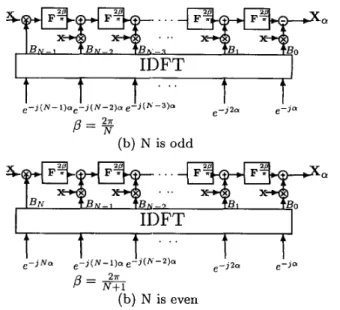
Eq. (24) shows us that the DFRFT with any angle can be realized by the DFRFT with only one special angle, and it can be implemented by the cascade method shown in Fig.3. Similar to the parallel method, the special angle

and numbers of terms of cascade forms are also different for the even and odd cases. The cascade form of the DFRFT in even case is written as:

2 P 2 P 2 8

X,

= F T ( . . . ( F " ( F ; T - ( B N X ~ + B N - I x ) + B N - z x ) + B N - - B x )

+

' . .)

+

Box (25) It can be observed that the structures in Fig.3 are very regular. So they are very suitable to be realized by the VLSI implementation.

Both the implementation methods can have the advan- tages for the DFRFT computation. The parallel method is suitable for the signal whose DFRFTs in special angles are already known. The computation of DFRFT will become only a linear combination of the DFRFTs in special angles. It has been shown in [1][6], a chirp signal can have an impulse output for a F R F T or DFRFT with a appro- priate angular parameter. So the F R F T and DFRFT can be used for the chirp signal detection. Using the proposed novel method, the DFRFTs of special angles of the desired signal can be computed in a priori. So the chirp signal can be detected easily.

In other way, the cascade method makes the computation of DFRFT can be realized from the DFRFT with only one specified angle. If the DFRFT with the specified angle can be computed efficiently, the computation of DFRFT will become efficient. Such an architecture is very suitable for the VLSI implementations.

5. C O N C L U S I O N S

In this paper, we develop a novel method for the DFRFT computation. By this new method, the DFRFT of any angle can be computed by the linear combination of the DFRFTs with special angles. The weighting coefficients of the linear combination are obtained from an IDFT computation. Moreover, this novel method can be realized by two methods: Parallel method and Cascade method. The parallel method is suitable for the signal whose DFRFT in special angles are already known. The chirp signal detection is a common one. And the cascade method is with regular structure, so it is very suitable for the VLSI implementation.

6. R E F E R E N C E S

L. B. Almeida, "The fractional Fourier transform and time-frequency representation," IEEE fians. Signal Process., vol. 42, pp. 3084-3091, Nov. 1994.

H. M. Ozaktas, B. Barshan, D. Mendlovic, and L. Onu- ral, "Convolution, filtering, and multiplexing in fractional Fourier domains and their relationship to chirp and wavelet transforms," J . Opt. Soc. Amer. A , vol. 11, pp. 547-559, Feb. 1994.

B. Santhanam and J . H. McClellan, "The discrete rota- tional Fourier transform," IEEE Trans. Signal Process.,

vol. 42, pp. 994-998, April 1996.

H. M. Ozaktas, 0. Arikan, M. A. Kutay, and

G.

Bozdagi, "Digital computation of the fractional Fourier transform," IEEE Trans. o n Signal Process., vol. 44, pp. 2141-2150, Sept. 1996.

(4)

[5] S. C. Pei and M. H. Yeh, “Improved discrete fractional Fourier transform,” Optics Letters, vol. 22, pp. 1047- 1049, July 15 1997.

[ 6 ] S. C. Pei, M . H. Yeh, and C. C. Tseng, “Discrete fractional Fourier transform based on orthogonal projec- tion,” IEEE Trans. Signal Processing, vol. 47, pp. 1335- 1348, May 1999.

[7] A . V. Oppenheim, Discrete-time signal processing. Prentice-Hall International Inc., 1989.

[8] C. Candan, M . A . Kutay, and H. M. Ozaktas, “The dis- crete fractional Fourier transform,” ZEEE Trans. Signal

Process., vol. 48, pp. 1329-1337, May 2000.

[9] D. F. Elliott and K .

R.

Rao, Fast Fourier transform and convolution algorithms. Springer-Verlag, 1982.

4 m t - 1 4 m + 2 4 m + 3 N

I

the eigenvalues 4m

I

e - J k a , k = 0 , 1 , 2 , . . . , ( 4 m - 2 ) , 4 m

I

e - 3 m a , k = 0 , 1 , 2 , . . . , ( 4 m - l ) , 4 m e--lku, k = 0 , 1 , 2 ; . . , 4 m , ( 4 m + 2 ) e-Jka, k=0,1,2,...,(4m+l),(4m+2)

Table 1: The eigenvalues assignment rule of DFRFT kernel matrix

I

N=5 Xm

t

N=6

Figure 1: The special angles that the DFRFT are evaluated

p = &

(a)

N

is odd

p = &

N+l

(b)

N

is even

Figure 2: The block diagrams for the parallel DFRFT implementation

p = Z

N+ 1

(b) N is

even

Figure 3: The block diagrams for the cascade DFRFT implementation