Subscriber access provided by NATIONAL TAIWAN UNIV
Industrial & Engineering Chemistry Research is published by the American Chemical Society. 1155 Sixteenth Street N.W., Washington, DC 20036
Article
Nonparametric Identification for Control of MIMO Hammerstein Systems
Jyh-Cheng Jeng, and Hsiao-Ping Huang
Ind. Eng. Chem. Res., 2008, 47 (17), 6640-6647 • DOI: 10.1021/ie071512q • Publication Date (Web): 30 July 2008
Downloaded from http://pubs.acs.org on November 18, 2008
More About This Article
Additional resources and features associated with this article are available within the HTML version: • Supporting Information
• Access to high resolution figures
• Links to articles and content related to this article
Nonparametric Identification for Control of MIMO Hammerstein Systems
Jyh-Cheng Jeng and Hsiao-Ping Huang*Department of Chemical Engineering, National Taiwan UniVersity, Taipei 106, Taiwan
A new nonparametric method to identify multivariable Hammerstein models is presented. The Hammerstein model is characterized by a combination of a linear dynamic subsystem and an algebraic nonlinear function. There could be many different models that give the same input-output realization. The purpose of this identification is to find out one among those models for controller design. This identification uses a sequence of specially designed test signals for excitation. The linear dynamic subsystem is identified as a finite sequence of impulse response (FIR), and the static nonlinearity is identified as a multi-input-multi-output (MIMO) functional mapping. By making use of this special test signal, the FIR sequence can be estimated under a single-input-single-output (SISO) framework. Moreover, the identification for linear subsystem can be decoupled from that for the nonlinear static part. This nonparametric model can be used for model predictive control applications.
1. Introduction
Most of the dynamics of chemical processes are nonlinear in nature. In order to be able to describe the global behavior of the system, many research activities have been focused on developing methods for modeling and identification of such nonlinear systems. One of the most frequently used nonlinear models is the Hammerstein model, which is composed of a nonmemory function as the static nonlinearity part followed by a linear dynamical subsystem. Because of this model structure, the model expressions of the process are not unique, especially, for multi-input-multi-output (MIMO) systems.
Many methods for modeling and identification of Hammerstein-type systems published in the open literature focused on the single-input-single-output (SISO) systems. Only a few exceptions dealt with the MIMO systems (e.g., Verhaegen and Westwick;1 Al-Duwaish and Karim;2Patwardhan et al.;3Rollins et al.;4 Laksh-minarayanan et al.5). The methods for identification of MIMO Hammerstein system differ mainly in the way the static nonlinearity is represented and the optimization problem finally formulated. In parametric approaches, the static functional nonlinearity is ex-pressed in terms of polynomials, neural networks, and some expansions of basis functions. A priori process knowledge is required to select an appropriate functional form. Regardless of the parametrization of system, the resulted optimization problem (sometimes nonconvex) is usually difficult to deal with, especially the global convergence of the estimated parameters. The use of Narendra-Gallman algorithm for the identification5,6allows the prediction error to be separately linear in each set of parameters that characterize the linear and nonlinear parts. But it requires iterative procedures and could lead to divergent results in some cases. To develop noniterative algorithms, particular basis functions have been used to represent the static nonlinearity,7,8and a linear regression problem for a parameter matrix containing product of the model parameters can be formulated. This parameter matrix is estimated with least-squares estimation, and the model parameters are then calculated by singular value decomposition of the parameter matrix. Although the optimization problem was simpli-fied, parametrization of static nonlinearity is still required. Recently, Lee et al.9proposed a method using a special test signal that enables decoupling the dynamic linear part and the static nonlinear part
for identification. But, it is applicable only to the case where nonlinearities are in terms of polynomial.
Motivated by the difficulties encountered in identifying an MIMO Hammerstein model, a new nonparametric method is presented in this paper. Parametrization of systems is not required, and complicated optimization problems are avoided. By using special test signals designed for this purpose, the identification of multivariable linear subsystem can be carried out under a SISO framework and can be decoupled from that of the static nonlinear function. As mentioned, due to the two-part structure of the process, models for input-output realization may not be unique; but they are all in equivalence. Among them, the one that has best linear dynamic characteristics could be used to develop the model predictive control for the process. In this paper, the identification as well as its application to model predictive control (MPC) will be illustrated.
2. Problem Formulation
A Hammerstein system is schematically represented as the one in Figure 1. The system consists of a static nonlinear function F(•) followed by a linear time-invariant (LTI) dynamic element G(q). Let H(l)∈ Rm×nwith elements {h
ij(l)}i)1,2,..., n;j)1,2,..., mbe the FIR matrix of G(q) and F(•):RmfRmbe a nonlinear vector functional mapping. The Hammerstein representation of the process is then given by y(k) )
∑
l)0 L-1 H(l)v(k - l) + e(k) v(k) ) F(u(k)) (1) where u(k), v(k)∈ Rm, y(k), and e(k)∈ Rn, are the system input, intermediate input, output, and noise, respectively. The constant L is the longest length among all of the impulse sequences, hij(l). Based on a series of input u(k) and output y(k), the identification problem is formulated as the one to find H(l) and F(•) that can predict yˆ(k), from u(k), with least sum of squared errors to the* To whom correspondence should be addressed. E-mail: huanghpc@
ntu.edu.tw. Tel: 886-2-2363-8999. Fax: 886-2-2362-3935. Figure 1. Structure of the Hammerstein model.
10.1021/ie071512q CCC: $40.75 2008 American Chemical Society
observation y(k). In this paper, the inputs are specially designed so as to enable sequentially estimations of H(l) and F(•). No parametrization for both the functional nonlinearity and the LTI element is required at this stage. The only assumptions needed are that the LTI element is stable and the nonlinear function has a value of zero at the origin, i.e., F(0) ) 0.
For simplicity, formulation is based on a 2 × 2 system. However, extension to a general m× m system is straightfor-ward without difficulty.
3. Identification of LTI Subsystem
If input and output data of a LTI linear MIMO system are available, a FIR matrix can be found using the linear least-squares (LS) method.10
Nevertheless, in such a Hammerstein system, input (i.e., v(k)) to the linear subsystem is dummy and not measurable. But, if the static nonlinear function is driven by a two-level signal switching between zero and a nonzero constant, the resulting v(k) will be a two-level signal between zero and another nonzero constant. By this way, the LS method can be applied to estimate the FIR sequence. For this reason, a specially designed test signal to excite the linear subsystem is thus required.
3.1. Process Excitation. The test signal is generated by
modulating each input with multistage inputs. In each stage, say stage J, uJ(k) is a pseudorandom binary signal (PRBS) which switches between zero and a nonzero constant in a random manner while keeping all other inputs being zero (i.e., uj(k) ) 0, j * J). The excitation signals are as shown in Figure 2. The number of such excitations equals the number of input variables. It follows that each dummy input (Vj(k), j ) 1,2,..., m) at the Jth stage is a PRBS switching between zero and a nonzero constant as well. Notice that each Vj(k) is synchronized to uJ(k).
As we will show in the following, such a test signal makes the identification of LTI element possible.
3.2. Estimation of FIR Matrix. Consider the LTI element
in a 2× 2 Hammerstein process. We denote a PRBS input that has levels at a and b as PRBS(a,b). The inputs at the first stage for excitation are u1(k) ) PRBS(uj1,0) and u2(k) ) 0. As a result, the intermediate inputs at this stage are
V
1(k) ) PRBS(f1(u1, 0), 0) V
2(k) ) PRBS(f2(u1, 0), 0) (2) Then, at the second stage, u1(k) ) 0, u2(k) ) PRBS(uj2,0) and thus we have
V
1(k) ) PRBS(f1(0, u2), 0)
V2(k) ) PRBS(f2(0, u2), 0) (3) The switch times of V1(k) and V2(k) is always synchronized to those of u1(k) and u2(k) in each of the two stages, respectively. The input-output relationship of eq 1 can be written, provided R1, R2* 0, as y(k) )
∑
l)0 L-1[
h11(l) h21(l) h12(l) h22(l)][
f1(u(k - l)) f2(u(k - l))]
)∑
l)0 L-1[
h11(l) R1 h21(l) R2 h12(l) R1 h22(l) R2]
[
R1f1(u(k - l)) R2f2(u(k - l))]
(4)Figure 2. Inputs for the identification of the LTI subsystem.
Figure 3. Inputs for the identification of static nonlinearity.
Figure 4. Realization model of the Hammerstein system.
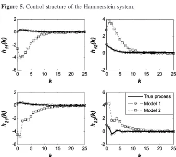
Figure 5. Control structure of the Hammerstein system.
Figure 6. Impulse response of LTI subsystem in example 1.
Equation 4 shows that the nonlinear functions in F(•) can be scaled by any nonzero constants because the LTI subsystem can compensate it accordingly. Thus, we can designate f1(uj1,0) as uj1and f2(0,uj2) as uj2, which means R1) uj1/f1(uj1,0) and R2) uj2/f2(0,uj2). Consequently, the dummy inputs at these two stages are defined as follows. At the first stage, V1(k) ) u1(k) and V2(k) ) p2u1(k), where p2) R2f2(uj1,0)/uj1. Similarly, at the second stage, V1(k) ) p1u2(k) and V2(k) ) u2(k), where p1) R1f1(0,uj2)/ uj2. Notice that the values of uj1and uj2are given by the excitation signals, while the values of p1 and p2 are parameters to be specified.
A 2× 2 input-output realization of the LTI element in eq 1) can be written as y1(k) )
∑
l)0 L-1 [h11(l)V1(k - l) + h12(l)V2(k - l)] + e1(k) y2(k) )∑
l)0 L-1 [h21(l)V1(k - l) + h22(l)V2(k - l)] + e2(k) (5) In the first stage, from eq 5, it becomesy1(k) )
∑
l)0 L-1 [h11(l) + p2h12(l)]u1(k - l) + e1(k) )∑
l)0 L-1 h1(1)(l)u1(k - l) + e1(k) y2(k) )∑
l)0 L-1 [h21(l) + p2h22(l)]u1(k - l) + e2(k) )∑
l)0 L-1 h2(1)(l)u1(k - l) + e2(k) (6)And, in the second stage y1(k) )
∑
l)0 L-1 [p1h11(l) + h12(l)]u2(k - l) + e1(k) )∑
l)0 L-1 h1(2)u2(k - l) + e1(k) y2(k) )∑
l)0 L-1 [p1h21(l) + h22(l)]u2(k - l) + e2(k) )∑
l)0 L-1 h2(2)u2(k - l) + e2(k) (7) where h1 (1) (l) ) h11(l) + p2h12(l) h2(1)(l) ) h21(l) + p2h22(l) h1(2)(l) ) p1h11(l) + h12(l) h2(2)(l) ) p1h21(l) + h22(l) (8) With eq 6, h1(1)(l) and h2(1)(l), for l ∈ [0,1,..., L - 1], can be obtained from a conventional SISO least-squares estimation10 with available data from (u1,y1) and (u1,y2) at the first stage. Similarly, with eq 7, h1(2)(l) and h2(2)(l) can be thus obtained with known data from (u2,y1) and (u2,y2) at the second stage. Rewrite eq 8 in matrix form as Q(l) ) H(l)P (9) where Q(l) )[
h1 (1)(l) h 1 (2)(l) h2(1)(l) h2(2)(l)]
H(l) )[
hh11(l) h12(l) 21(l) h22(l)]
P )[
1p p1 2 1]
(10) So H(l) ) Q(l)P-1, l ) 0, 1, . . . , L - 1 (11) Since the elements in Q(l) are estimated, the impulse response matrix H(l) can be computed by eq 11, provided that values of p1and p2are given. Notice that the product of p1and p2must not equal to 1 (i.e., the matrix P cannot be singular).Remark. A practical issue for FIR identification is the number
of data that should be used to arrive at an accurate model. PRBS has a pulse-like autocorrelation function which closely ap-proximates the delta function from an ideal white noise. Thus, least-squares identification using PRBS can result in a model with similar accuracy to that resulted from white noise excita-tion. Furthermore, if the data number (N) is an integer multiple of the period of the PRBS, then the pulse-like autocorrelation function still results, even when the number of data points is relatively small.11According to our experience in this study, N is chosen as an integer multiple of the period of the PRBS with N > 5L, where L is the length of FIR to be estimated.
4. Identification of Nonlinearity
With a set of given values of p1and p2, (denoted as p˜1and p˜2), the FIR matrix of the LTI subsystem is estimated by eq 11 as
H
˜(l) ) Q(l)P˜-1
(12) The obtained H˜ (l) and output y(k) can then be used to compute
the unobserved intermediate variable, v˜(k), that corresponds to the given u(k). With a sufficient number of such cor-respondence u(k) and v˜(k) data pairs, it will be able to establish a nonlinear functional mapping between the two variables by interpolation.
4.1. Excitation for Static Nonlinearity. In order to define
the nonlinear functional relationship between u(k) and v˜(k), the above-mentioned u(k) must cover the whole possible space of input variables. In addition, higher density of data pairs has to be used in the region where high model accuracy is desired. If there is not enough a priori knowledge about the process, signal with uniform density in the whole region is recommended. For this purpose, if the numbers of levels of u1and u2for excitation are n1and n2, respectively, then the test signal contains a total of n1× n2pairs which are all the combinations of values of u1 and of u2. Notice that each pair lasts for one sampling interval only. For example, u1 ) {-1,0,1} and u2) {-2,-1,0,1,2}, then there are 15 pairs in the test signal as shown in Figure 3. The sequence of these steps can be randomly ordered.
4.2. Estimation of Nonlinear Mapping. Assume the
intro-duced multistep signal contains n + 1 steps, i.e., u(k), k ) 0, 1,..., n, and u(k) ) 0 for k > n. Then, based on H˜ (l) and v˜(k), the LTI subsystem of eq 5 can be rewritten in a matrix form:
η ) Φ˜υ˜ + e (13) where Φ ˜ )
[
Φ˜11 Φ˜12 Φ ˜ 21 Φ˜22]
, υ˜ )[
υ˜υ˜1 2]
, η )[
ηη1 2]
, e )[
ee1 2]
(14) with Φ ˜ ij)[
h ˜ ij(0) 0 · · · 0 h ˜ ij(1) h˜ij(0) · · · 0 l l ·· · l h ˜ ij(n) h˜ij(n - 1) · · · h˜ij(0) l l ·· · l h ˜ ij(n + L - 1) h˜ij(n + L - 2) · · · h˜ij(L - 1)]
, h˜ij(l) ) 0 for l g L υ ˜j) [V˜j(0) V˜j(1) · · · V˜j(n) ]T ηi) [yi(0) yi(1) · · · yi(n + L - 1) ]T ei) [ei(0) ei(1) · · · ei(n + L - 1) ]TNotice that if the LTI element has time delay, the all-zero rows in Φ˜ and η have to be removed. Since the row number of
Φ˜ is always larger than the column number and all elements of Φ˜ are identified, we can now estimate the unobserved
inter-mediate variableυ˜ by the method of least-squares, i.e. υ
˜ ) (Φ˜TΦ˜ )-1Φ˜Tη (15) Thus, the nonlinearity is identified as the mapping from u(k) to
v˜ (k) thus obtained, that is, F˜ (•):u(k) f ν˜^ (k). Notice that we also have two known points of F˜ (uj1,0) ) [uj1p˜2uj1]Tand F˜ (0,uj2) ) [p˜1uj2uj2]T.
Having the FIR sequence and the nonlinear function, it will be able to predict the output from the given input, u(k). The model up to this stage has been identified. In general, this nonlinear function may be represented by an artificial neural network for interpolations. Or, it can be modeled as a multi-variable polynomial with cross terms. For example, consider
the nonlinear mapping to be represented by multivariable polynomials with order M as the following:
ν˜ˆi) f i ˆ(u1, u2;θi) )
∑
j)0 M θi,ju1M-ju2j (16)The parameters can be estimated by regression
θi/) arg min θi
∑
k)0 n
{fˆ(ui 1(k), u2(k);θi) -ν˜ˆi(k)}2 (17)
Remarks. According to eq 13, n + L data points are used
for the identification of nonlinearity. The selection of n may depend on the complexity of the nonlinearity, the range of the operating region, and the desired model accuracy.
4.3. Measurement Noise. If the noise e is random and white,
ν˜^ in eq 15 is an unbiased estimate of υ˜. Moreover, if the
number of rows in Φ˜ approaches infinity, ν˜^ is a consistent estimate ofυ˜. To increase the row number of Φ˜ , we can proceed
to test using the signal of which the steps are identical to those of previously used input, but the sequence is randomly scrambled. In this way, more equations for the unknownυ˜ can
be set up in eq 13 and hence a more consistent estimate ofυ˜
could result. However, this is at the cost of prolonged experiment time. In case of strong noise level, it is suggested that the measurement is first passed through a filter to reduce the effect of noise and maintain accurate identification of model without extra test. Another way to deal with the noise is fitting the estimated data set with a nonlinear function because the noise will be filtered out by the fitting procedure.
5. Tuning Matrix P˜ for Model-Based Control
According to the identification algorithm presented in sections 3 and 4, the resulting Hammerstein model is given in Figure 4 in a nonparametric form. In this model, the LTI element consists of two blocks, Q(l) and P˜-1, where Q(l) is defined by several identified SISO FIR sequences. Based on the given P˜ , the associated intermediate variable v˜ is estimated and then a nonlinearity F˜ (•) results accordingly. Generally, the values of p˜1and p˜2can be arbitrarily given (provided p˜1p˜2* 1), so that these two components of a MIMO Hammerstein model are not unique. In other words, for a given input-output set, many combinations of different static nonlinearity F˜ (•) and LTI
subsystem H˜ (l) may have identical outputs. Therefore, it gives engineers the flexibility to choose a model representation for better control. In the proposed model shown in Figure 4, this flexibility is achieved by selecting the values at the off-diagonal entries of P˜ . By a proper selection of this P˜ matrix, parametric models are developed for model-based control uses.
A control structure for Hammerstein type nonlinear process is as shown in Figure 5, where GCcan be a conventional PID controller or an MPC controller.12Assume the nonlinearity F˜ (•) is invertible so that the design of GCdepends only on H˜ (l). Thus, the off-diagonal elements of P˜ can be determined to meet
the desired characteristic imposed on the LTI subsystem H˜ (l). Two cases with different purposes of design are discussed in the following:
Steady-State Decoupling. If the system is square, the matrix P˜-1can be aimed to serve as a steady-state decoupler for Q(l), i.e., the LTI subsystem H˜ (l) is “self-decoupled” at steady state. Let Ki(j))∑l)0L-1hi(j)(l) be the steady-state gain of the dynamics described by hi(j)(l) and K be the steady-state gain matrix of
Q(l) in eq 10 with
K )
[
K1(1) K1(2)
K2(1) K2(2)
]
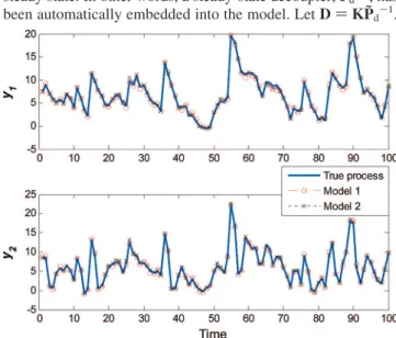
(18) By eq 12, if P˜ is chosen as P˜dsuch that KP˜d-1is a diagonal matrix, the linear subsystem described by H˜ (l) is decoupled atsteady state. In other words, a steady-state decoupler, P˜d-1, has been automatically embedded into the model. Let D ) KP˜d-1.
Figure 8. Process and model outputs to random input in example 1
Figure 9. Output response to multistep inputs in example 2.
The off-diagonal elements of P˜dare obtained by solving the equation
{Dij}i)1,2, . . . ,n;j)1,2, . . . ,m;i*j) 0 (19) For a 2× 2 system, the resulting P˜dis
P
˜ d)
[
1 K2(1)/K2(2)
K1(2)/K1(1) 1
]
(20)Diagonal Dominance. The diagonal dominance of a MIMO
model is usually desired because it means slight interactions between loops, so that the design of multiloop decentralized controller would be easier. To this end, the off-diagonal elements of P˜ can be estimated by solving the following optimization
problem to reduce the loop interactions {p˜1/, p˜2/} ) arg min p ˜1,p˜2
(
w1 |h˜ 12|2 |h˜11|2 + w2|h ˜ 21|2 |h˜22|2)
(21) where w1and w2are weighting factors of two loops and h˜ij) [h˜ij(0) h˜ij(1) · · · h˜ij(L - 1) ]T. Alternatively, similar to steady-state decoupling, P˜ can also be estimated to maximize thediagonal dominance of the LTI model at a certain frequencyω by letting P ˜ dd)
[
1 K2(1)(ω)/K2(2)(ω) K1(2)(ω)/K1(1)(ω) 1]
(22) where Ki(j)(ω) )|
∑
l)0 L-1 hi(j)(l)e-jlω|
Remark. As mentioned, the nonparametric input-output
realization model of Hammerstein process is not unique. The model can be made unique if a priori knowledge about the LTI element in terms of transfer function matrix is incorporated. For example, the linear elements in the LTI subsystem is of ARX form with known order (rij,sij) and delay dij, i.e.
Gij(q) )yVi(t) j(t) )Bij(q)q -dij Aij(q) )(bij,0+ bij,1q -1+ b ij,2q -2+ · · · + b ij,sijq -sij)q-dij 1 - aij,1q-1- aij,2q-2- · · · -aij,r
ijq
-rij (23)
The corresponding FIR sequence, for l > (dij+ sij) satisfies the following relation:
hij(l) ) aij,1hij(l - 1) + aij,2hij(l - 2) + · · · + aij,r
ijhij(l - rij) (24) Thus, the off-diagonal elements of P˜ can be determined such that the condition in eq 24 is satisfied. Although the parameters aijare unknown, they can be computed from h˜ij(l) by the method of least-squares, if the off-diagonal elements of P˜ are given.
That is
aij) (ΓijTΓij)-1ΓijTφij (25) where
aij) [aij,1 aij,2 · · · aij,rij] T φij) [h˜ij(dij+ sij+ 1) h˜ij(dij+ sij+ 2) · · · h˜ij(L) ] T Γij)
[
h ˜ ij(dij+ sij) h˜ij(dij+ sij- 1) · · · h˜ij(dij+ sij- rij+ 1) h ˜ ij(dij+ sij+ 1) h˜ij(dij+ sij) · · · h˜ij(dij+ sij- rij+ 2) l l ·· · l h ˜ ij(L - 1) h˜ij(L - 2) · · · h˜ij(L - rij)]
Notice that φij, Γij, and aij are functions of the off-diagonal elements of P˜ . Thus, these off-diagonal elements can be determined by solving an optimization problem. For example, a 2× 2 system, it is {p˜1/, p˜2/} ) arg min p ˜1,p˜1(
∑
i)1 2∑
j)1 2 |φ ij- Γijaij|2)
(26) As a result, a unique representation of the Hammerstein model is obtained. If the model order and delay are unknown, the above optimization problem can be solved repetitively using different sets of (rij,sij,dij) until the residual is smaller than required.6. Simulation Example
Example 1. Consider a nonlinear process described by the
Hammerstein system as follows:
G(q) )
[
0.1q-1+ 0.2q-2 1 - 1.2q-1+ 0.35q-2 q-1 1 - 0.7q-1 0.3q-1+ 0.2q-2 1 - 0.8q-1 q-1+ 0.5q-2 1 + 0.4q-2]
F(u) )[
u1 3- u 1u2+ 2u2 2 0.582(e(u1+u2)- 1)]
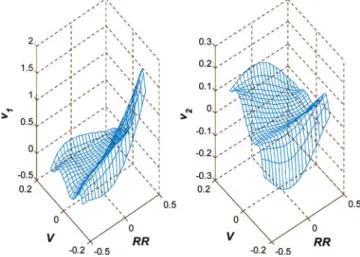
Figure 11. Plot of nonlinearity in example 2.
Figure 12. Process and model outputs to random input in example 2.
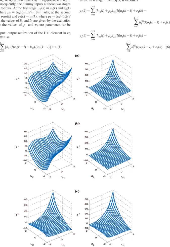
The inputs for estimation of FIR matrix are chosen as u1(k) ) PRBS(1,0), u2(k) ) 0 at the first stage and u1(k) ) 0, u2(k) ) PRBS(1,0) at the second stage. The input for identification of the nonlinearity is a multivariable multistep signal which covers all the combination of u1) u2) {-2:0.2:2}, i.e., a total of 21× 21 ) 441 pairs. The sampling interval is taken as 1. To simulate the measurement noise, random white noise is added to the output, with|e1(k)| e 0.2 and |e2(k)| e 0.2. First, the matrix Q(l) is identified from the PRBS test. Here, two models with different characteristics for the LTI subsystem are used for illustration. First, the order (rij,sij) of ARX dynamics for the LTI subsystem is assumed known (model 1). The results obtained by eq 26 are p˜1) 1.973 and p˜2) 0.965. Notice that their exact values are p1) 2 and p2) 1. In the second one, steady-state decoupling is imposed on the LTI subsystem (model 2), and the results computed from eq 20 are p˜1) 0.592 and p˜2 ) 1.357. The impulse response sequences of these two models together with that of original process are shown in Figure 6. Based on the two LTI models, two corresponding input-output mappings of the nonlinearity are thus estimated from the test of multistep signal. These mappings have been fitted with multivariable polynomials as shown in Figure 7. The outputs of original Hammerstein system and two identified models to random input are simulated as shown in Figure 8. As mentioned previously, although these two representations of the Hammer-stein model are quite different, both of them can produce very similar outputs to that of the original system.
Example 2. Consider a distillation column with 30 trays for
the separation of a binary mixture as it was used by Benallou et al.13 and Horton et al.14 The column is described by 32 nonlinear ordinary differential equations and is assumed to have a constant molar overflow as well as a constant relative volatility of 1.6. The feed stream is introduced at the middle of the column on stage 17 and has a composition of xF) 0.5. The reflux ratio (RR) and the vapor boilup (V) are the input variables (u1and u2), and the distillate composition (xD) and bottom composition (xB) are used as output variables (y1and y2). The steady-state values of these four variables are RR ) 3, V ) 0.8, xD) 0.935, and xB) 0.065.
The proposed method is used to identify a Hammerstein model based on simulation data with a sampling time of 10s. The operating region for this system was chosen to be (15% around the steady-state vales. The exciting signals for the estimation of FIR matrix are u1(k) ) PRBS(0.225,0), u2(k) ) 0 at the first stage and u1(k) ) 0, u2(k) ) PRBS(0.06,0) at the second stage. Then, a multivariable multistep signal which covers all the combination of u1) {-0.45:0.045:0.45}, u2) {-0.12:0.012:0.12} is used to estimate the nonlinearity. Colored noises, w(k), with autoregressive dynamics of order 1 (i.e., w(k) ) 0.8 w(k - 1) + e(k)) are added to the outputs to simulate a more realistic scenario. The noise-to-signal ratio (NSR), defined as the following, is around 20%.
NSR ) mean (abs (noise)) mean (abs (signal))
The output response to multistep inputs is shown in Figure 9. Based on the excitation of PRBS, the matrix Q(l) is first identified. We assume that all dynamics of the LTI subsystem are represented as ARX of order (1,1) without time delay, and the parameters are found as p˜1 ) -0.213 and p˜2 ) -0.014. The identified impulse response sequences are shown in Figure 10. Based on this LTI model, the corresponding input-output mappings of the nonlinearity are thus estimated from the test of multistep signal. This mapping has been fitted with multi-variable polynomials of order 5, as shown in Figure 11. The simulated response of the identified Hammerstein model is compared with the actual response in Figure 12, where a good agreement between them can be observed. For the purpose of comparison, random signals covering the operating region were used to excite the process, and a linear model (FIR matrix) is thus identified using the least-squares estimation. The simulated response of the identified linear model is also shown in Figure 12. Clearly, the predictive capability of the Hammerstein model outperforms that of the linear model.
Example 3. To demonstrate that different model
representa-tions can be used for nonlinear control application, a Hammer-stein process with simple nonlinearity as follows is considered.
G(q) )
[
-0.112q-1- 0.058q-2 1 - 1.05q-1+ 0.136q-2 0.59q-1 1 - 0.607q-1 0.85q-1 1 - 0.717q-1 0.098q-1 1 - 0.95q-1]
F(u) )[
u1 2+ 2u 2 2u1- u22]
The operating region is u1, u2 ∈ [-1 1], and the sampling interval is 1. Three identified Hammerstein models with different characteristics for the LTI subsystem (i.e., ARX of known order, steady-state decoupling, and diagonal dominance) are used for the nonlinear MPC design given in Figure 5. The control horizon and prediction horizon are taken as 2 and 5, respectively, in all simulations. Each input and output is equally weighted. The closed-loop responses are shown in Figure 13. It can be seen that all the identified models can be used for control design with satisfactory responses. Nevertheless, better control perfor-mance is found when the model with diagonally dominant dynamics for the LTI subsystem is used.
7. Conclusion
In this paper, a new method has been presented to identify and model MIMO Hammerstein systems. By the proposed special test inputs, the identifications of LTI subsystem and nonlinearity are separated, so that iterative procedures are avoided. Because the proposed method is a nonparametric one, the parametrization of system is not required in advance and
thus the representation of model is not unique. With the identified nonparametric realization of the system, engineers can have the flexibility in modeling Hammerstein systems to meet their demands by adjusting a few parameters. Simulation results have shown that an accurate model can be identified by the proposed method. Furthermore, different model representations can be used to describe the behavior of a Hammerstein system and can be used for control design.
Note Added after ASAP Publication: The version of this
paper that was published on the Web July 30, 2008 has errors in it that were associated with eq 2. The corrected version of this paper was reposted to the Web August 5, 2008.
Literature Cited
(1) Verhaegen, M.; Westwick, D. Identifying MIMO Hammerstein Systems in the Context of Sub-Space Model Identification Methods. Int. J.
Control 1996, 63, 331–349.
(2) Al-Duwaish; Karim, M. N. A New Method for the Identification of Hammerstein Model. Automatica 1997, 33, 1871–1875.
(3) Patwardhan, R. S.; Lakshminarayanan, S.; Shah, S. L. Constrained Nonlinear MPC Using Hammerstein and Wiener Models: PLS Framework.
AIChE J. 1998, 44, 1611–1622.
(4) Rollins, D. K.; Bhandari, N.; Bassily, A. M.; Colver, G. M.; Chin, S. T. A. Continuous-Time Nonlinear Dynamic Predictive Modeling Method for Hammerstein Processes. Ind. Eng. Chem. Res. 2003, 42, 860–872.
(5) Lakshminarayanan, S.; Shah, S. L.; Nandakumar, K. Identification of Hammerstein Models Using Multivariate Statistical Tools. Chem. Eng.
Sci. 1995, 50, 3599–3613.
(6) Eskinat, E.; Johnson, S. H.; Luyben, W. L. Use of Hammerstein Models in Identification of Nonlinear Systems. AIChE J. 1991, 37, 255– 268.
(7) Gomez, J. C.; Baeyens, E. Identification of Block-Oriented Nonlinear Systems Using Orthonormal Bases. J. Process Control 2004, 14, 685–697. (8) Chan, K. H.; Bao, J.; Whiten, W. J. Identification of MIMO Hammerstein Systems Using Cardinal Spline Functions. J. Process Control
2006, 16, 659–670.
(9) Lee, Y. J.; Sung, S. W.; Park, S.; Park, S. Input Test Signal Design and Parameter Estimation Method for the Hammerstein Wiener Processes.
Ind. Eng. Chem. Res. 2004, 43, 7521–7530.
(10) Hsia, T. C. System Identification: Least-Squares Methods; D.C. Heath and Co.: Lexington, MA, 1977.
(11) Sung, S. W.; Lee, J. H. Pseudo.Random Binary Sequence Design for Finite Impulse Response Identification. Control Eng. Practice 2003,
11, 935–947.
(12) Fruzzetti, K. P.; Palazoglu, A.; McDonald, K. A. Nonlinear Model Predictive Control Using Hammerstein Models. J. Process Control 1997,
7, 31–41.
(13) Benallou, A.; Seborg, D. E.; Mellichamp, D. A. Dynamic Com-partmental Models for Separation Processes. AIChE J. 1986, 32, 1067– 1078.
(14) Horton, R. R.; Bequette, B. W.; Edgar, T. F. Improvements in Dynamic Compartmental Modeling for Distillation. Comput. Chem. Eng.
1991, 15, 197–201.
ReceiVed for reView November 7, 2007 ReVised manuscript receiVed May 15, 2008 Accepted May 23, 2008
IE071512Q