A Novel MPEG-Analytic Approach to Video Segmentation for Video Data Organization and Retrieval

全文

(1)A Novel MPEG-Analytic Approach to Video Segmentation for Video Data Organization and Retrieval Mu-Ke Yang (楊木科) and Wen-Hsiang Tsai (蔡文祥) Department of Computer & Information Science National Chiao Tung University 1001 Ta Hsueh Rd., Hsinchu, Taiwan 300, R. O. C. Tel: 886-3-5712121 Ext. 56650 Email: gis89582@cis.nctu.edu.tw researches about video segmentation have been conducted in the past decade. The main idea of video segmentation is to find cuts, which are frames with abrupt changes in contents. Cuts can be found by sequentially tracing a video stream and comparing every two successive images, until abrupt content changes are found. Equivalently, the sequence of frames between two cuts is just a shot mentioned previously. Therefore, we also call video segmentation as shot change detection or cut detection. Existing video segmentation methods can be generally categorized into two major approaches [1]: segmentation in the uncompressed domain and that in the compressed domain. Proposed methods for segmentation in the uncompressed domain can be further grouped roughly into two categories: pixel comparison and histogram comparison. A method of the former category compares the intensity/color values of corresponding pixels in two successive frames in given videos [8, 9]. And a method of the latter category compares the absolute sum of the histogram differences between two successive video frames [8-10]. It is tried in such methods to reduce the sensitivity of the segmentation results to object movements and camera operations. It is known that two images that include the same background and moving objects with little shape changes will have similar histograms. This is the principle behind such methods of the histogram-comparison approach. Generally speaking, this approach yields better video segmentation results than the pixel-comparison approach. Recently video data are mostly produced and kept in the compressed format to save the storage space. A lot of video segmentation researches are focused on creating effectively compressed videos. The Moving Picture Exert Group (MPEG) standard is very widely used in compressing video data. The main concept of segmentations in the compressed domain is to segment videos by MPEG features. Three types of features are generally used to segment videos: (1) discrete cosine transform (DCT) coefficients; (2) macro-block codes, and (3) motion vectors. Arman et al. [11] proposed first a technique for shot detection using the DCT coefficients in the I frames of videos. Zhang et al. [12] applied a pair-wise comparison technique to the DCT. Abstract Video data organization and retrieval are useful in many applications in today’s digital world. For this purpose, a novel MPEG-analytic two-phase method for video segmentation to construct video information systems is proposed. In the first phase, a video is first segmented into rough shots using certain MPEG features specially selected in this study. The rough shots are then merged into more meaningful ones by a technique of histogram comparison in the second phase. Experimental results show the feasibility and practicability of the proposed method.. 1. Introduction A. Motivation Recently digital video data become more and more popular in many applications. Various applications related to video data have been implemented, such as digital libraries, distance learning, videos on demand, etc. However, video data are usually huge in size and the processing time for them is often very long. In order to manage video data efficiently, a convenient video information system must be provided. Generally speaking, when people search video data in a video information system, they usually look for specific image frames and shots, instead of searching for a certain video in a set of videos. As a result, the main goal of video segmentation is to cut video streams into numerous meaningful shots as the basic unit. After segmentation of a video, a reference frame needs to be extracted from each resulting shot to represent the shot. It is desired to propose an effective video segmentation method for this purpose. B. Survey of Related Studies To achieve the aims of efficient keeping, management, indexing, retrieval of video data, as well as providing good user interfaces [1-4], a convenient and versatile video information system is desired. Recently, many researches have been conducted on the development of techniques related to such a kind of video system, such as the OBIC of IBM [5], the OVID [6], the CORE [7], etc. The first step of constructing a video information system is video segmentation. A plenty of related 1.

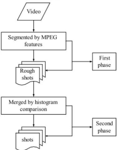
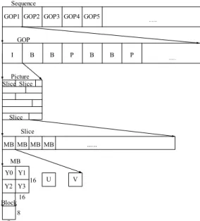
(2) the shots obtained in the first phase as input, and compute the differences of the histograms between every two successive start frames. When the difference is smaller than a threshold, it means the two frames are similar, and we merge the two corresponding shots then. Figure 1 shows a flowchart of the proposed segmentation method.. coefficients of corresponding blocks of I frames. Yeo and Liu [13] proposed a DC coefficient based algorithm to detect scene changes. This reduces greatly the data size for the detection process. Meng et al. [14] proposed a shot change detection algorithm based on the use of the DC coefficients and the MB coding modes. Liu and Zick [15] presented a technique based on the error signal and the number of motion vectors. Gamaz et al. [16] proposed a skipping algorithm for fast and accurate detection of abrupt scene changes in videos. Pei and Chou [17] proposed a method that uses macroblock (MB) information of MPEG-compressed video bitstreams to analyze and segment videos. They exploited comparison operations performed in a motion estimation procedure, which results in specific characteristics of MB-type information when scene changes occur or when some special effects are applied. Comparing the above two categories of algorithms, one can find that video segmentation methods in the compressed domain have more advantages than those in the uncompressed domain. Some of such advantages are described in the following. First, since segmentation in the compressed domain does not need decoding of the video stream, it can save the decompression time and the storage space of the decompressed images. Next, the segmentation work can be performed faster because the size of the compressed data is smaller than that of the uncompressed data. Furthermore, each compressed video contains a rich set of features that can be used as measures to detect shots. And finally, videos are gradually stored in the compressed format, especially in the MPEG format. Therefore, conducting video segmentation directly in the compressed domain is more practical, as is done in this study.. Video. Segmented by MPEG features. Rough shots. First phase. Merged by histogram comparison Second phase. shots. Figure 1 Flowchart of the segmentation method. B. Review of MPEG Standard The MPEG standard is widely used for video compression. The standard defines syntax, semantics, and the decoding mode of a compression bit stream. It utilizes two basic techniques to reduce redundancy: (1) use of macro-block based motion compensation to reduce the temporal redundancy in videos; (2) use of the discrete cosine transform (DCT) to reduce the spatial redundancy in videos. In this section, we will give a brief review of the MPEG standard. (1) Structural Hierarchy of MPEG The structural hierarchy of the MPEG standard shown in Figure 2 is divided into six layers, namely, the sequence layer, the group of pictures (GOP) layer, the picture layer, the slice layer, the macroblock (MB) layer, and the block layer. We will explain the structure and contents of each of the layers in the sequel. The sequence layer is the top-level layer of the The sequence layer is the top-level layer of the MPEG stream; it contains parameters of encoding and continuous GOP layers. The GOP layer consists of different types of encoded pictures (frames), including intra-coded (I) pictures, predictive-coded (P) pictures, and bi-directionally predictive-coded (B) pictures. This layer generally includes one I picture, a number of P pictures, and a number of B pictures. Two parameters M and N are flexibly set by an encoder to determine the structure of the GOP. The distance between two P pictures is given by M and the length of a GOP is given by N. A typical GOP like IBBPBBPBBPBBPBB has the parameters M equal. 2. Overview of Proposed Method and Review of MPEG Standard A. Overview of Proposed Method We mentioned previously that segmentation in the compressed domain has more advantages. Therefore, we propose in this study a new segmentation method that can be employed to find rough shots in the compressed domain, and refine shots by merging in the uncompressed domain. With such a process of two stages, we name our method a two-phase video segmentation method. In the first phase, we take an MPEG video as input, and analyze the MPEG coding features. We define some measures for every type of frame to determine which frame could be a cut. When the dissimilarity measure of a frame with respective to the preceding one is larger than a threshold, we decide this frame to be a cut and decode it into an uncompressed image. We call this image the start frame of a shot. In the second phase, we use the start frames of all 2.

(3) chrominance components. Since humans are sensitive to luminance, it is appropriate to take less samples of chrominance to reduce data storage . The ratios of the three types of blocks are generally Y : U : V = 4 : 1 : 1. It means that four blocks share a U block and a V block in an MB.. to 3 and N equal to 15. The use of the GOP is intended to assist random access into the MPEG stream. Sequence GOP1 GOP2 GOP3 GOP4 GOP5. ....... (2) Reduction of Spatial Redundancy The main technique of reduction of the spatial redundancy in videos is the DCT. The DCT has been adopted in many compression standards, such as MPEG, H261, H263, JPEG, etc. The function of the DCT is to transform data of the spatial domain into the frequency domain. With the DCT, the energy will concentrate at positions of low frequencies, and the coefficients of high frequencies will tend to be zero. Subsequent quantization is performed to make the coefficients of high frequencies tend to become zero to increase the overall compression ratio. In the MPEG compression, a block of the size of 8×8 pixels is used as the basic unit to perform the DCT. The equation for the 2D DCT is. GOP I. B. B. P. B. B. P. ....... Picture Slice Slice. Slice Slice MB MB MB MB. ....... MB Y0 Y1 Y2 Y3 Block. 16. U. V. 16 8. 8. Figure 2 Structural hierarchy of the standard MPEG.. F (u , v) =. (1). The picture layer consists of several slices decoded separately to avoid influence on the whole frame during error decoding. The length of a slice is decided by the encoder. The MB layer is the most important layer in the MPEG stream. The MB is an elementary unit to perform motion compensation. There are four types of MB modes in this layer. They are intra-coded MB (IMB), forward-coded MB (FMB), backward-coded MB (BMB) and bi-directionally-interpolated MB (BIMB). Every picture coding type consists of different MB coding modes. The relationships between picture coding types and MB coding modes are listed in Table 1. Encoders use the MB as the unit to calculate motion compensated prediction errors to determine the type of the MB coding mode. If the type of a MB is FMB, BMB or BIMB, it needs to perform motion prediction to obtain motion vectors. If the type of the MB is IMB, it just uses the DCT to encode the data itself.. where  1  C (u ), C (v) =  2  1. FMB ˇ ˇ. BMB. BIMB. 8*8 Block. ˇ. for u, v = 0, 0, otherwise;. f(x, y) represents the pixel at coordinates (x, y) in the original image. The first DCT coefficient F(0, 0) is called the DC coefficient and is 8 times the average intensity of the respective block. The other coefficients are called AC coefficients. IMB’s are coded by the DCT using the data in the picture of itself. The quantization (Q) and zigzag coding is applied to the transformed block to reduce the number of bits and organize the block for run length encoding (RLE). The Q converts most of the high frequency components to zero, maintaining the least error in the encoding of low frequency components. The zigzag scanning organizes the quantized data to a 1-D coefficient sequence suited for RLE. Finally, the Huffman coding is used to encode the sequence into bit streams. The encoding process of IMB’s is shown in Figure 3.. Table 1 The relationship between picture coding types and MB coding modes IMB I pictures ˇ P pictures ˇ B pictures ˇ. 7 7 1  (2 x + 1)uπ   (2 y + 1)vπ  C (u )C (v)∑∑ f ( x, y ) cos   cos   4 16 16     x = 0 y =0. ˇ. DCT. Quantiza tion. Zigzag. RLE. Huffman Bit Coding stream. Figure 3 Encoding process of IMB. (3) Reduction of Temporal Redundancy With high similarity in adjacent frames in videos, many redundant data in frames can be exploited. Therefore, MPEG compression uses motion compensation to reduce temporal redundancy. A. The block layer is the lowest layer in the MPEG stream. The size of a block is 8×8 pixels. The block is the elementary unit to perform the DCT. An MB contains 4 blocks of three types: Y, U, V blocks. Y is the luminance component; and U and V are the 3.

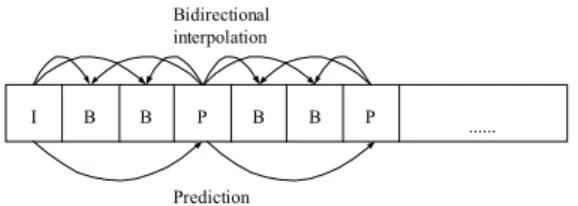
(4) choose the DC coefficient of each block in an I frame as the measure to determine if a cut occurs in the frame. More specifically, we compute the sum of the differences of the DC coefficient values in all blocks between two I successive frames to determine if a cut occurs in the first frame. For comparing the two I frames we adopt the equation proposed in [16]. It’s a normalized average of the absolute difference of DC coefficients. The dissimilarity measure D(fm, fn) between two I frames fm and fn is defined to be:. 16×16 MB is adopted as the elementary unit for motion compensation. During the encoding process, the encoder finds the most similar reference MB in the reference frame and calculates the motion vector. P pictures are coded with forward motion compensation using the nearest previous reference (I or P) pictures. B pictures are coded with forward, backward, or interpolated prediction with respect to both future and past reference pictures. Figure 4 shows a typical GOP and the predictive relationships between different types of pictures. Bidirectional interpolation. I. B. B. P. B. D( fm, fn) =. B. P. Prediction. Figure 4 Typical GOP and predictive relationships between I, P and B pictures When decoding the P or B pictures, each MB in pictures could be intra-coded or inter-coded. Therefore, the encoder must perform motion estimation to determine which MB coding mode should be adopted and use different methods to encode. After motion estimation, if the motion compensation prediction error (MCPE) is larger than a threshold, it means that the difference between the two MB’s is large and the encoder will choose the intra-coded mode to encode; otherwise, if the MCPE is smaller than the threshold, the encoder will choose the inter-coded mode. Figure 5 shows the process of coding mode decision.. 16*16 Motion MB estimation. | c( fm,i ) − c( fn,i ) |. i =1. m. (2). n. B. Shot Change Detection in P Frames P frames are different from I frames; they are not all intra-coded. They cannot be employed to detect cuts using the DC coefficient data because of the lack of complete DCT coefficients. Some MB’s in P frames are inter-coded. They are FMB’s. Each FMB uses the reference MB in a reference frame (an I or P frame) to predict the DCT coefficients. As a result, we detect cuts in P frames using the MB coding types. We define a measure Dp to represent the degree of dissimilarity of a P frame to its reference frame (denoted by R) and another measure DPi to represent the dissimilarity of an MB with index i (denoted as MBi) in the P frame to its corresponding one in the reference frame R. If the MB coding mode of an MB in the P frame is IMB, it implies that it is dissimilar to the corresponding MB at the same position in the reference frame R. For this case, we set the value Dpi equal to 1. If the MB coding mode of MBi in the P frame is FMB, it implies that the MB is similar to the MB at the same position in R, or similar to an MB with a shifted position in R with an offset specified by a motion vector with respective to R. In such a case, for finer detection we do not set Dpi equal to 0 directly. Instead, we also consider the similarity contributed by the so-called coded block pattern (CBP). The CBP is used to determine whether or not it is necessary to store the difference of a block in an MB with respect to a corresponding block in the reference frame. In a standard MPEG compression format, an MB contains six blocks in which four are Y blocks, one is a U block, and the last is a V block. When an MB is created by motion prediction, the. Intercoded. MCPE computation >T. k. ∑ max(c( f ,i), c( f ,i)). where c(fI, i) is the DC coefficient of block i in frame fI, and k is the number of blocks in an frame. When D(fm, fn) is larger than a threshold T1, it implies the difference between two successive frames is great and we decide that the frame is a suspended cut. When a frame is decided to be a suspended cut, it means that the frame could be a cut, but another measure of a B frame need be computed to determine if the suspended cut is a real cut.. ....... <T. 1 k. Intracoded. Figure 5 Process of MB coding mode decision.. 3. Details of Proposed Video Segmentation Techniques In the proposed video segmentation method, some techniques are utilized to accomplish the segmentation, including detections of shot changes in I, P, and B frames. The basic concepts of these techniques will be described in this section. We will also explain how to merge shots by the technique of histogram comparison here. A. Shot Change Detection in I Frames Since all MB’s in I frames are intra-coded, each MB contains complete DCT coefficient data. We can use DCT coefficients to detect shot changes in I frames. Since the DC coefficient is eight times the average intensity of the respective block, we just 4.

(5) we decide that the frame is a real cut. If a P frame or an I frame is decided to be a suspended cut, we need another similarity measure of a B frame to determine if the suspended cut is a real cut or if a cut occurs at a B frame. We define the measure SB to represent the similarity degree of a B frame to its backward reference frame (denoted as BR) and SBi to represent the similarity measure of an MB in the B frame (denoted as MBi). If the MB coding mode of MBi is BB, it implies that MBi is similar to the corresponding MB in the backward reference frame BR. For this case, we set the value of SBi to 1. BIMB’s, IMB’s and FMB’s are not created relatively to a backward P or I frame, so we set the value SBi of a BIMB, IMB or FMB to 0. Finally, we sum up again all the values of SBi to compute the value SB of the B frame by the following equation:. encoding process not only finds the similar MB in the reference frame, but also computes the motion vectors and the differences values between the two blocks. The CBP is a binary number with six bits. Each bit in the CBP represents whether the difference between the corresponding the blocks need be transmitted. If a bit of the CBP is 1, it implies that the block is a little different from the block in the reference MB. For this reason, when the an MB in a P frame is an FMB, we first consider the CBP value. Let n be the number of 1’s appearing in the CBP. Then, we set the dissimilarity measure DPi of this FMB to its corresponding MB in the reference frame R to be (1/2)×(n/6). Finally, we sum up all DPi to compute the value of DP of the P frame according to the following equation:. Dp =. 1 k ∑ Dpi k i =1. (3) SB =. where k is the total number of MB’s in the P frame. When the value of Dp is larger than a threshold T2, we claim that the frame is a suspended cut. If a P frame is claimed to be a suspended cut, another measure of a B frame need be computed to determine if the suspended cut is a real cut, as described next.. DB =. 1 ∑ DBi k i =1. (5). where k is the total number of MB’s in the B frame. When the value of SB is larger than a threshold T3, we decide that the B frame is a real cut, otherwise, we decide instead the suspended cut to be a real cut. D. Shot Merging by Histogram Comparison In the shot change detection in I, P, or B frames, we compare the block information at identical positions in two frames. Therefore, the techniques of the first segmentation phase are based on the template-matching concept. A drawback of template-matching based techniques is that the results of shot change detection will be sensitive to camera operations and object movements. As a result, some superfluous shots might be detected. As a remedy, we compare further the start frames of every two successive shots by their color histograms to merge superfluous shots when certain conditions are met. The details are as follows. We first define a similarity measure DH(Si, Si+1) to compare the start frames Si and Si+1 of shots i and i+1, respectively in the following way:. C. Shot Change Detection in B Frames We define two measures for shot change detection in B frames. One is for forward detection like the measures described in the preceding section; and the other determines if the suspended cut is a real cut. The main concept of the first measure for shot change detection in B frames is similar to that of the measure for shot change detection in P frames. We define similarly a dissimilarity measure DB to represent the dissimilarity degree of a B frame to its reference frame (denoted as R) and another dissimilarity DBi to represent the dissimilarity measure of an MB (denoted as MBi) to its corresponding one in R. The dissimilarity measures for an IMB and an FMB in a B frame are defined similarly to those for a P frame. We set the value DBi of an IMB to 1, and that of an FMB to n/12. Since BIMB’s and BMB’s are created relatively to a backward reference frame and since the concept of the proposed dissimilarity measure is to determine if the frame is similar to the preceding frame, we set the value DBi of a BIMB or a BMB to 0. Finally, we again sum up the values of all DBi to compute the value of DB of the B frame by the following equation: k. 1 k ∑ SBi k i =1. DH(Si, Si+1) =. n −1. ∑ ∑| H (S , j) − H (S c. i. c. i +1 ,. j) |. (6). c∈{R ,G , B} j =0. where Hc(Si, j) is the value of the histogram of color c for level j in the start frame Si, and n is the number of levels. If DH(Si, Si+1) is smaller than a threshold T4, it means that the two shots are similar, and we merge them into a single shot.. 4. Detailed Algorithm for Segmentation Process. (4). In this section, we will give detailed descriptions of the algorithms for the proposed segmentation process.. where k is the total number of MB’s in the B frame. When the value of Dp is larger than a threshold T2, 5.

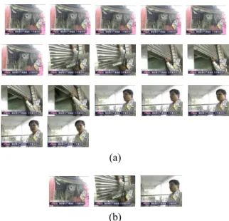
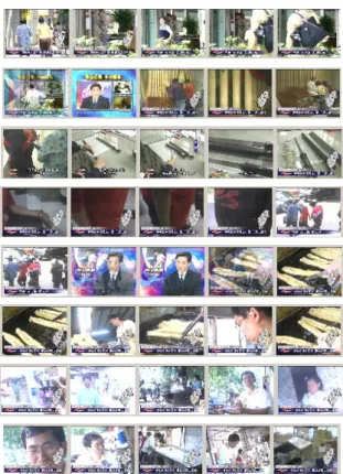
(6) The following algorithm is a summary of the proposed video segmentation process.. A. Phase of Rough Segmentation into Shots First, we take a video as input and analyze it. In an MPEG video stream, an input frame sequence is generally formed by three types of frames in a special order such as:. Algorithm 1. Video segmentation into shots by MPEG features. Step 1: Input a video V and decode it into a frame sequence of three picture coding types. Let the sequence be:. 1I 4P 2B 3B 7P 5B 6B 10P 8B 9B 13I 11B 12B 16P 14B 15B …. It is worth to mention that P frames are decoded before B frames according to the MPEG standard. The reason is that P frames are used to be the reference frames for B frames, so they must be decoded first. But the actual output frame sequence of the decoder is:. 1I (1+M)P 2B 3B … MB (1+2M)P (M+2)B (M+3)B … (2M)B (1+3M)P (2M+2)B (2M+3)B … (3M)B … (1+l*M)P … (1+k*N)I …… Step 2: Decode the picture coding type of the current frame. If the type is I, go to Step 3. If the type is P, go to Step 4. And if the type is B, go to Step 5. Step 3: Compute the measure D(f1+(k−1)*N, f1+k*N) of the (1+k*N)I frame. If the value of the measure is larger than T1, go to Step 6; else, go to the next frame and repeat Step 2. Step 4: Compute the measure DP of the (1+l*M)P frame. If DP is larger than T2, go to Step 7; else, go to the next frame and repeat Step 2. Step 5: Compute the measure DB of the (l*M+m)B frame. If DB is larger than T2, take this B frame as a real cut; else, go to the next frame and repeat Step 2. Step 6: Examine if any cut occurs between f1+(k−1)*N and f1+k*N. If the result is negative, go to Step 7; else, go to the next frame and repeat Step 2. Step 7: Compute the measures SB of the (l*M+2)B (l*M+2)B … ((l+1)*M)B. If the measure SB of a certain (l*M+m)B is larger than T3, take (l*M+m)B as a real cut; else, take the I or P frame as a real cut. Go to Step 2.. 1I 2B 3B 4P 5B 6B 7P 8B 9B 10P 11B 12B 13I 14B 15B 16P …. This action is called frame reordering. When the frame coding type is I, we use Equation (2) to compute the measure D(fm, fn). If the measure D(fm, fn) is larger than T1 and no cut occurs between fm and fn, we decide that the I frame is a suspended cut. We have to compute the measure SB of the next B frame by Equation (5) to determine if a cut really occurs at this I frame or at the next B frame. We use the video sequence mentioned in the previous paragraph as an example. When the computed D(f1, f13) is larger than T1, we must compute the measures SB of 11B and 12B. If the computed measure SB of 11B and that of 12B are both larger than T3, it means that at 11B an obvious shot change occurs, and a real cut may be put there. If the measure of SB of 11B is smaller than T3 and that of 12B is larger than T3, it means that 12B is a real cut. If the measure of SB of 11B and that of 12B are both smaller than T3, it means that both 11B and 12B are not similar to 13I and we may decide that 11I is definitely a real cut. When the frame coding type is P, we use Equation (3) to compute the measure DP. If DP is larger than T2, then we decide that the P frame is a suspended cut. We have to compute the measure SB of the next B frame by Equation (5) to determine if a cut occurs at this I frame or at the next B frame. We again use the video sequence mentioned previously as an example. When the computed value of Dp of P4 is larger than T2, we must compute the measures of SB of 2B and 3B. If the measure SB of 2B and that of 3B are both larger than T3, it means that at 2B a shot change occurs, and a real cut may be put there. If the measure of SB of 2B is smaller than T3 and that of 3B is larger than T3, it means that 3B is a real cut. If the measure of SB of 2B and that of 3B are both smaller than T3, it means that neither 3B nor 4B is similar to 4P and we may decide that 4P is definitely a real cut. When the frame coding type is B, we use Equation (4) to compute the measure DB of the B frame. If the value of DB is larger than T2, then we decide that the B frame is a real cut.. Figure 6 shows a flowchart of the proposed segmentation process using MPEG features. The thresholds T1, T2, and T3 are determined experimentally. As an example of experimental results of applying Algorithm 1, Figure 7(a) shows a sequence of video frames extracted from a news video segment, and Figure7(b) shows the resulting shots with each shot being represented with a reference frame (the first frame in the shot). B. Phase of Shot Refinement by Merging After the first phase of segmentation, we continue to perform the second phase of shot refinement by merging using color histogram comparison as mentioned previously While detecting a cut in the first phase, we decode and save it as a start frame of a shot. In the second phase, we compare the color histograms of consecutive start frames of neighboring shots to reduce superfluous shots by merging. 6.

(7) As revealed by these examples, people will regard the frames in each group (in Fig. 8(a) or 8(b)) to be similar, but the segmentation algorithm of the first phase does not yield such results. Therefore, we propose the second-phase algorithm for refinement of such unreasonable shots by merging.. Video V. Decode V into a frame sequence of three picture coding types. I N. Y. Picture coding type?. N. B N. P. Calculate D(fm, fn). Calculate DP. Calculate DB. D(fm, fn)>T1. DP>T2. DB>T2. Y. Y. Cuts occur between fm and fn. Y A cut occurs at the B frame.. N Calculate SB. (a). SB>T3. Y. N A cut occurs at the previous I or P frame.. A cut occurs at the B frame.. Figure 6 Flowchart of video segmentation process by MPEG features. (b) Figure 8 Some examples of start frames of superfluous shots caused by camera operations and object movements. We use the technique of histogram comparison mentioned previously to determine if the start frames Si and Si+1 of two given successive shots i and i+1, respectively, are similar. First, we use Equation (5) to calculate the measure DH(Si, Si+1) of the two start frames. If DH(Si, Si+1) is smaller than a threshold T4, it means that shots i and i+1 with the two given start frames Si and Si+1 are similar, and we then merge the two shots. The following algorithm is a summary of the proposed refinement process based on histogram comparison.. (a). (b) Figure 7 Example of experimental results of video segmentation into shots. (a) A given video frame sequence. (b) Shots obtained from applying Algorithm 1 (each shot represented by the start frame of the shot).. Algorithm 2. Shot refinement by merging using histogram comparison. Step 1: Input the start frames S1, S2, …, Sn of all the shots that are segmented out by the segmentation algorithm of the first phase (Algorithm 1). Step 2: Compute the measure DH(Si, Si+1) of the start frames Si and Si+1 of every two successive shots i and i+1. If DH(Si, Si+1) is smaller than T4, then merge the two shots; else go to next start frame and repeat Step 2 until all start frames are examined.. Superfluous shots are created by the template-matching based algorithm from frame content changes caused by sensitivity of camera operations or object movements. Figure 8 illustrates some examples of start frames of superfluous shots caused by camera operations and object movements. 7.

(8) Although some false detections did appear, the statistics show that the proposed method is acceptable from an overall viewpoint of effectiveness.. As an example of experimental results using Algorithm 2, Figure 9 shows two shot refinement results with the two groups of frames in Figure 8 as inputs.. (a). (b). Figure 9 Two results of shot refinement by Algorithm 2 with Figures 8(a) and 8(b) as inputs, respectively.. 5. Experimental Results A lot of videos were tested in our experiments using a PC with a Pentium IV and 1.4G CPU and a 384MB RAM. And software development was conducted by the use of Visual C++ 6.0 and Borland C++ 5.0 in a Windows 2000 Professional platform. Some segmentation results have been shown previously. Here, we concentrate on reporting the segmentation correctness of the proposed method. The videos used in the experiment contains several ones that were collected from two cable TV channels: TVBS and ET. Two metrics Precision and Recall are defined as follows to measure the correctness of the video segmentation results: Precision=. NC , Recall= NC NC + NF NC + NM. Figure 10 Part of the results of segmentation with TVBS news video on 2002/03/21 as input.. (7). where NC is the number of correct shot change detections, NF is the number of the false shot change detections, and NM is the number of the missed shot change detections. The numbers NC, NF and NM are all decided by visual inspection. We randomly chose some segments from TVBS news videos and ET news videos as the test videos. Some statistics of the experimental results of video segmentation are listed in Table 2, including the total number of frames, the numbers of correct, false, and missed detections, the precision values, and the recall values in a video. Figure 10 shows part of the results of segmentation with a TVBS news video on 2002/03/21 as input. We saw from our experimental results that abrupt shot changes were almost all detected by Algorithm 1. And some shots caused by camera operations or object movements can be eliminated by Algorithm 2. However, if the camera zooms, booms, tracks, dollies, or pans too quickly in some frames, false cuts will be detected. Besides, the proposed method almost does not miss shot changes because the recall values in Table 2 are almost 100%.. Table 2. Statistics of experimental results of video segmentation. Video. TVBS segment 1 TVBS segment 2 TVBS segment 3 ET Segment 1 ET segment 2. No. of Correct False Missed Precision Recall frames detections detections detections. 6275. 36. 6. 1. 89%. 95%. 6001. 38. 5. 0. 88% 100%. 6360. 36. 3. 0. 92% 100%. 6527. 38. 8. 0. 82% 100%. 9655. 80. 15. 2. 84%. 97%. 6. Conclusions A shot is the elementary unit for video retrieval, so successful video segmentation is an essential step of video data organization and retrieval. A novel video segmentation method has been proposed in this study. The method uses two phases to segment a video into shots based on some effective MPEG features in the first phase and to merge similar shots by histogram comparison in the second phase. The 8.

(9) segmentation and merging steps are based on several similarity measures defined in this study in terms of specially selected features coming from various types of MPEG codes of image frames. The method has been applied to real news video streams and the statistics of the experimental results show the feasibility of the method.. International Conference on Multimedia, pp. 267-272, 1993. [12] H. J. Zhang, C. Y. Low, Y. H. Gong, and S. W. Smoliar, “Video parsing using compressed data,” Proceedings of SPIE Conference on Image and Video Processing II, pp. 142-149, 1994. [13] B. L. Yeo and B. Liu, “A unified approach to temporal segmentation of motion JEPG and MPEG compressed videos,” Proceedings of International Conference on Multimedia Computing and Systems, Vol. 2, pp. 330-334, 1996.. References [1] F. Idris and S. Panchanathan, “Review of image and video indexing techniques,” J. of Visual Communication and Image Representation, Vol. 8, No. 2, pp. 146-166, 1997.. [14] J. Meng, Y. Juan, and S-F. Chang, “Scene change detection in MPEG compressed Video sequence,” Digital Video Compression: Algorithms and Techniques, SPIE, Vol. 2419, pp. 14-25, 1995.. [2] I. Koprinska and S. Carrato, “Temporal video segmentation: A survey,” Signal Processing: Image Communication, Vol. 16, pp. 477-500, 2001. [3] C. W. Chang and S. Y. Lee, “Video content representation, indexing and matching in video information systems,” J. of Visual Communication and Image Representation, Vol. 8, No. 2, pp. 107-120, 1997.. [15] H. C. H. Liu and G. L. Zick, “Scene decomposition of MPEG compressed video,” Digital Video Compression: Algorithms and Techniques, SPIE, Vol. 2419, pp. 16-37, 1995. [16] N. Gamaz, X. Huang and S. Panchanathan, “Scene change detection in MPEG domain,” Proceedings of IEEE Southwest Symposium on Image Analysis and Interpretation, pp. 12-17, 1998.. [4] G. Amato, G. Mainetto, and P. Savino, “An approach to a content-based retrieval of multimedia data,” Multimedia Tools and Applications, vol. 7, pp 9-36, 1998. [5] M. Flickner, et al., “Query by image and video content: the QBIC system,” IEEE Computers, Vol. 28, pp. 23-32, 1996.. [17] S. C. Pei and Y. Z. Chou, “Efficient MPEG compressed video analysis using macroblock type information,” IEEE Transactions on Multimedia, Vol. 1, No. 4, pp. 321-333, 1999.. [6] E. Oomoto and K. Tanaka, “OVID: design and implementation for a video-object database system,” IEEE Trans. on Knowledge and Data Engineering, Vol. 5, No. 4, pp 629-643, 1993. [7] J. k. Wu, et al., “CORE: a content-based retrieval engine for multimedia information system,” Multimedia Systems, Vol. 3, No. 1, pp 25-41, 1995. [8] A. Nagasaka and Y. Tanaka, “Automatic video indexing and full video search for object appearance,” IFIP: Visual Database Systems II, pp. 113-127, 1995. [9] H. J. Zhang, A. Kankanhalli, S. W. Smoliar, and S. Y. Tan, “Automatic partitioning of fullimotion video,” ACM Multimedia Systems, pp. 10-28, 1993. [10] Y. Tonomura, “Video handling based on structured information for hypermedia systems,” ACM Proceedings: International Conference on Multimedia Information Systems, pp. 333-344, 1991. [11] F. Arman, A. Hsu, and M.-Y Chiu, “Image processing on compressed data for large video databases,” Proceedings of First ACM 9.

(10)