Power Efficient Topology Control in Wireless Ad
Hoc Networks
Chih-Cheng Tseng*
Graduate Institute of Communication Engineering, National Taiwan University,
Taipei, Taiwan, R.O.C. [email protected]
Kwang-Cheng Chen
Graduate Institute of Communication Engineering, National Taiwan University,
Taipei, Taiwan, R.O.C. [email protected] Abstract—In the wireless ad hoc networks, for prolonging the
communication duration of the nodes, the transmission power is required to be minimized to conserve the limited battery life. In addition, for the wireless ad hoc networks to be applicable, the networks are required to be connected. Unfortunately, the two requirements are against each other. In this paper, by analyzing the probability of isolated node, we obtain the relationships between transmission range, service area and network connectedness. Furthermore, we propose a generalized (N,B) wireless ad hoc network model to investigate the impact of boundary nodes on the network connectivity, equivalent service area and average node degree.
Keywords-ad hoc networks, connectivity, power conservation I. INTRODUCTION
Wireless ad hoc network is a self-organizing network architecture that is rapidly deployable and adapts to the propagation conditions and to the traffic and mobility patterns of the network nodes. Possible examples of the wireless ad hoc networks are tactical military applications, disaster recovery operations, exhibitions or conferences. Due to the characteristics of lacking fixed infrastructure and all the communications are carried over the wireless medium, nodes are usually mobile. As a consequence, the power source is mainly supplied by batteries. To prolong the communication duration of the nodes, the transmission power must be minimized so as to conserve the limited battery life. However, for a wireless ad hoc network to be applicable, the network is required to be connected, i.e. given any two nodes in the network, there must exist at least one path to connect these two nodes. Unfortunately, it is contradiction between power conservation (shorter transmission range is preferred) and network connectivity (longer transmission range is preferred) in designing wireless ad hoc network. Our first objective, in this paper, is to propose a solution to compromise these two issues. One of the first researches on this topic is examined in the context of a “broadcast percolation” in [1]. For broadcast percolation in one spatial dimension, analytical expressions for the average extent of percolation are derived and a model for two-dimensional spatial percolation is presented along with related simulation results. They also suggested that the choice of optimal transmission radius might be bounded from below by the need to maintain desired network connectivity. In [2], if nodes are distributed according to a two-dimensional Poisson
point process with density D, then, in an infinite area there exists an infinite connected component with nonzero probability if the expected number of nearest neighbors of a transmitter N0 is bounded by 2.195<N0<10.526. In addition,
they also conjectured that transmission range for connectivity and covering are the same. However, Piret in [3] proved that in one-dimensional, the transmission range problem and the covering problem may exist at different range and, further, they conjectured that even in two-dimensional, these two problems are also different. Based on two different mobility models, Santi and Blough in [4] studied the relationship of the transmission range to maintain connectivity between the cases of stationary and mobility during some fraction of the operational time. They concluded that (i)it is not the mobility models but the “quantity of mobility”, which can be informally defined as the percentage of stationary nodes with respect to the total number of nodes influences the connectedness most and (ii)if brief periods of disconnection are allowed and/or only a significant fraction of the nodes being connected, the transmission range can be reduced largely. Gupta and Kumar [5] considered the problem of placing n nodes randomly and independently in a disc of unit area in R2 and showed that if
log ( )
2( ) n c n
n
r n
π = + , then the resulting network is asymptotically
connected with probability one if and only if c n( )→ +∞. Similar results are obtained in [6]. Recently, Bettstetter [7] employed the nearest neighbor method to study the range assignment problem. He assumed the distribution of nodes as a homogeneous Poisson point process in R2 and obtained the minimum transmission range for the network to be connected. Besides, [7] also employed the results on the geometric random graph [8] to obtain the transmission requirements to generate a
k-connectivity wireless ad hoc network. Based on the work in
[7], our approach uses the uniform node distribution to simplify the analysis of minimum transmission range and network connectivity. The second objective of this paper is to study the impact of boundary nodes on the network connectivity. Based on a proposed generalized ( , )N B wireless ad hoc network model, the maximum number of boundary nodes for the network to maintain connectivity and the corresponding minimum average node degree are obtained.
The rest of this paper is organized as follows: Section II provides criterion to achieve the optimum transmission range and network connectedness. In Section III, we generalize the
*C-C Tseng is also with the Department of Electronic Engineering,
connectivity and average node degree problems to an ( , )N B connected wireless ad hoc network model. Simulations and results are presented in Section IV and Section V concludes the paper.
II. OPTIMUM TRANSMISSION RANGE AND NETWORK CONNECTEDNESS
In this section, given the maximum network service area and the minimum required probability of no isolated node in an
N nodes wireless ad hoc network, we provide the transmission
range lower bound for the network to be connected and the probability for the network to be connected. We also provide conditions to ensure a deployed wireless ad hoc network to be fully connected by deriving a probability upper bound for the wireless ad hoc network to have no isolated node. With the results proved by Penrose [8], this probability upper bound provides the criterion for the network to be connected.
A. Preliminary
The entire network is assumed as an undirected graph
G(V,E), where V is the set of nodes with cardinality N, i.e., V={1,2,…,N} and E is the set of edges E={(i,j):i,j∈V}. Every node v in the set V is assigned an unique ID which is denoted by the numbers 1,2…,N. Furthermore, it is assumed that edges are all bi-directional and the transmission range for each node is fixed and identical. Thus if (i,j) is an edge between node i and node j, then so is (j,i) between node j and node i. We assume that all packets are exchanged over an error-free wireless channel. We also define the following terminologies. The degree of a node is the number of one-hop neighbors that the node connects with. A node with degree 0 is said to be an
isolated node and a node with degree 1 is regarded as a
boundary node.
B. Probability of Isolated Nodes
For a wireless ad hoc network to be connected, it is necessary to prevent the generation of isolated nodes since the isolated nodes partition the entire network into set of independent and disconnect sub-networks. Assume nodes in the wireless ad hoc networks are uniformly distributed over an equivalent service area A with the probability density function
1
A
f = A. Then, for a given node, the probability that there are
i nodes among the rest of N-1 nodes within its transmission
radius R is formulated as a binomial distribution with the parameter q πR A2
= and, thus, the average node degree is
(
) (
)
2 1 1 Pr , 1 1 . N average k R d k k N N A π − = =∑
− = − (1)According to the definition of the isolated node, the probability of an isolated node in a wireless ad hoc network with N nodes is equivalent to the probability that a node without any neighbor within its transmission range. Thus, we have
(
) (
)
2 1 Pr isolated node =Pr 0, 1 1 . N R N A π − − = − (2)Assuming statistical independence applies, the probability of no isolated node in an N nodes wireless ad hoc network, i.e. the minimum node degree in the network is greater than 1,
min 1 d ≥ , is
(
)
(
)
(
)
(
)
min Pr no isolated node Pr 1 1 Pr 0, 1 N. d N = ≥ = − − (3)Based on (3), if the probability of no isolated node in an N nodes wireless ad hoc network is required to greater than p, the transmission range R will be lower bounded by
(
)
1 1 1 1 1 . N N p R A π − − − ≥ (4)Since the transmission range is proportional to the transmitting power, (4) provides us an alternative to efficiently utilize the minimum power to satisfy the required network design parameters. Another variation of (3) is that if the minimum requirement of p and R are given, the upper bound of the equivalent service area A to satisfy p and R will be
(
)
1 1 1 2 . 1 1 N N R A p π − ≤ − − (5)C. Connectedness of A Wireless Ad Hoc Network
A graph is said to be k-connected if for each node pair in the graph there exist at least k mutually independent paths connecting them [9]. In other words, if (k-1) nodes fail, the graph is still guaranteed connected. The connectivity of a graph
G, written κ( )G , is the minimum size of a separating set S such that G S− is disconnected or has only one vertex. In (3), we have obtained the probability of no isolated node in a wireless ad hoc network. However, to achieve connectedness, a question arises “Is a wireless ad hoc network with no isolated node equivalent to a connected wireless ad hoc network?” The answer to this question is obviously no!! According to the graph theory, if a graph G is a simple graph, then
min
( )G d ( )G
κ ≤ [9], i.e., a wireless ad hoc network with no isolated node is only the necessary condition for a wireless ad hoc network to be connected. Thus, we have
( )
(
)
(
min)
Pr κ G =k ≤Pr d ≥k . (6)
For example, the graph G in Figure 1, ( ) 1κ G = ,
min( ) 3
d G = . For (6) to be useful, we need to know the tightness of the upper bound. With the geometric random graph proposition stated in [7] and [8], Penrose proved that with very high probability, under large enough node N, a k-connected geometric random graph is organized when the minimum degree dmin = in which links between nodes are added as R k
increases. In other words,
( )
(
)
(
min)
Pr κ G =k =Pr d ≥k . (7)
for Pr d
(
min ≥k)
almost one.Based on (7), we provide Theorem 1 as the criterion for the network to be k-connected and, by letting k=1, we obtain Theorem 2 as the requirement for the network is connected.
Theorem 1: For a wireless ad hoc network with N nodes,
each with transmission range R and uniformly distributed in an equivalent service area A, the probability that the network is k-connected is
(
) (
min)
1(
)
0 Pr -connected =Pr 1 Pr , 1 . N k i k d k − i N = ≥ = − − ∑
(8)Theorem 2: For a wireless ad hoc network with N nodes,
each with transmission range R and uniformly distributed in an equivalent service area A, the probability that the network is connected is
(
)
(
)
min1 2
Pr connected Pr no isolated node Pr( 1)
1 1 . N N d R A π − = = ≥ = − − (9)
III. ANALYSIS OF AN ( , )N B CONNECTED WIRELESS AD HOC NETWORK
An ( , )N B connected wireless ad hoc network is a connected wireless ad hoc network with B boundary nodes among the total network nodes N. This network scenario often occurs when nodes are sparsely spread and connected over the entire service area. For instance, the sensor network spreads sensors or data collectors in a forest to collect certain statistics. An example of (6,5) connected wireless ad hoc network is illustrated in Figure 2.
Based on the network model, we first analyze the average coverage area of an ( , )N B connected wireless ad hoc network. In general, with perfect channel assumption, the coverage of a node with transmission range R can be modeled as a circle with radius R. In this case, the minimum coverage area of an ( , )N B
connected network Amin is obtained when the (N B− ) non-boundary nodes are overlapped altogether and all the B boundary nodes connect to the overlapped nodes as the example shown in Figure 2. To simplify our analysis, the minimum coverage area of an ( , )N B connected network is approximated as a hexagon and the minimum coverage area
is 2
min 3 3 2
A R . To derive the maximum coverage area of an ( , )N B connected wireless ad hoc network, we construct the ( , )N B connected wireless ad hoc network by the following steps. First, generates a connected virtual backbone with
(N B− ) nodes. Then, for each of the B boundary nodes, randomly selects a node in the virtual backbone to connect with. It is easy to verify that any boundary nodes in the constructed ( , )N B connected wireless ad hoc network always located within the coverage of the virtual backbone. In other words, boundary nodes do not extend the coverage area of the ( , )N B
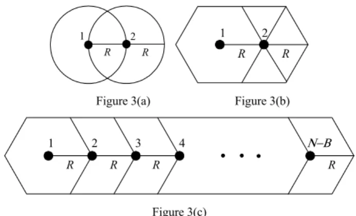
connected wireless ad hoc network. Thus, the maximum coverage area of the ( , )N B connected wireless ad hoc network is equivalent to the coverage area of the virtual backbone. Now, consider the case for a N B− = virtual backbone. For 2 this backbone to be connected, these two nodes must be within the transmission range of each other. Consequently, the maximum coverage area of a 2-node virtual network is shown in Figure 3(a). The corresponding hexagonal approximation is shown in Figure 3(b). In this case, the maximum coverage area can be approximated by (1 2 3)+ AH where AH is the area of a
hexagon with radius R. Figure 3(c) shows the approximated maximum coverage area Amax for a general ( , )N B connected
wireless ad hoc network and the maximum coverage area is
(
)
max 2 1+ 1 . 3 H A N B− − A (10)Since nodes are assumed to be uniformly distributed over the coverage area, i.e.
[
Amin,Amax]
, the average coverage area of an ( , )N B connected wireless ad hoc network, Aavg, is(
)
1 2 (2 1 . 2 3 avg H A = + N B− − A (11)It is obvious in (11) that Aavg increases as N increases or B
decreases. If the service area of the considered ( , )N B
connected wireless ad hoc network is Aservice, the equivalent service area A of the network is bounded by
{
}
min service, avg ,
A= A kA (12)
R
Figure 2 The minimum coverage area of a (6,5) connected network.
1 2
R R
1 2
R R
Figure 3(a) Figure 3(b)
1 2 R 3 R 4 R R Ν−Β Figure 3(c)
Figure 3 The approximated maximum coverage area of an ( , )N B connected
where k≅1.2 is the scaling factor from hexagon back to circle.
In the following, we provide two lemmas as the preliminary of Theorem 3 for finding the upper bound of the number of boundary node and the lower bound of the average node degree of an ( , )N B connected wireless ad hoc network.
Lemma 1: The necessary condition for a wireless ad hoc
network with more than two nodes to be connected is that there exists at least one node with degree>1.
Proof: If a wireless ad hoc network with more than 2 nodes
is complete (i.e. every node pair is adjacent), the proof is trivial!! Otherwise, for a wireless ad hoc network to be connected, it must exist at least one path with length>2 (i.e. there are more than two links constitute the path) between any random selected two nodes that are not connected directly. This means that there exists at least one intermediate node that the path traverses. In other words, there exists at least one incoming link and one outgoing link at the intermediate node resulting in the intermediate node with degree>1.
Lemma 2: A connected wireless ad hoc network with no
loop has the minimum average node degree.
Proof: Consider a connected wireless ad hoc network is
organized by adding node one by one into a network that is empty initially. Since the resulting average node degree is required to be minimum, each added node needs to introduce minimum number of degree. This can be achieved by connecting the added node to only one node in the constructing network, i.e., only one link is established at a time. Since only one link is introduced whenever a node is added, there is no loop in the constructed wireless ad hoc network. In other words, the resulting no loop network has the minimum average node degree.
Theorem 3: For an ( , )N B wireless ad hoc network to be
connected, the maximum number of boundary node, Bmax, is
bounded by (N− and the minimum average node degree is 1) bounded by 2Bmax N .
Proof. From Lemma 1, we know that there, at least, must
exist a non-boundary node for a wireless ad hoc network to be connected. In other words, the maximum number of boundary nodes Bmax in a connected wireless ad hoc network with N
nodes is (N− . From Lemma 2, we know that the minimum 1) average node degree is obtained when the network is built without loop. In connected wireless ad hoc network with N nodes, the number of links to connect these N nodes without loop is (N− . Since a link connects two nodes increases the 1) total network degree by two, the average node degree is
max
( 1)
2 N 2B .
N− = N
Following, we analyze the impact of boundary node on the average node degree D of an ( , )N B connected wireless ad hoc network. We first compute the average node degree of the virtual network of (N B− ) nodes dvb
(
1)
2 . vn R d N B A π = − − (13).Then, to construct an ( , )N B connected wireless ad hoc network, we further need B links to connect the B boundary nodes to the constructed virtual network. Hence, the average node degree of an ( , )N B connected wireless ad hoc network is
(
) (
)
2 1 1 R 2 . D N B N B B N A π = − − − + (14) 0 10 20 30 40 50 60 0 40 80 120 160 200 240 280 320 360 400 Tx Range A verage N ode D egree Ana. (N=200) Ana. (N=300) Ana. (N=400) Sim. (N=200) Sim. (N=300) Sim. (N=400)Figure 4 The average node degree without considering the border effect.
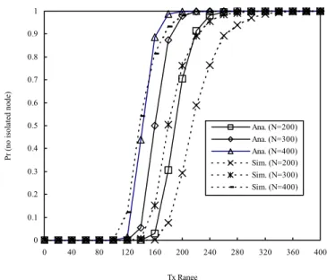
0 0.1 0.2 0.3 0.4 0.5 0.6 0.7 0.8 0.9 1 0 40 80 120 160 200 240 280 320 360 400 Tx Range
Pr (no isolated node)
Ana. (N=200) Ana. (N=300) Ana. (N=400) Sim. (N=200) Sim. (N=300) Sim. (N=400)
Figure 5 Probability of no isolated node in an N nodes wireless ad hoc network without considering the border effect.
IV. SIMULATION AND RESULTS
We verify our analyses by conducting extensive simulations coded in C language. We first to verify the probability of no isolated node obtained in (3) by uniformly placing N nodes into a service area of
2
(Terrain_X Terrain_Y)m
service
A = × . We assume that
Terrain_X = Terrain_Y = 2000. Figure 4 shows the average node degree as derived in (1) and Figure 5 shows the probability of no isolated node as derived in (3). It is obvious that there is a significant difference between the simulation results and the analytical results. This difference is mainly
because the simulation area we considered is a bounded area. In a bounded area, nodes that located near by the border are more likely to have fewer neighbors. This problem is so-called “border effect.”
To this problem, we modify the solution proposed in [10] by extending an area with width of R around the borders of the original bounded area. The resulted simulation area is depicted in Figure 6. We call the extended area as border area Aborder and
the original area as inner area Ainner. We define the node density
α as the average number of nodes per unit inner area i.e.
inner N A
α= and, then, generate pseudo nodes uniformly among the area Aborder based on the node density α. Now, for
R
A
inner
A
border
R (R,R) (Terrain_X+R, Terrain_Y+R) (Terrain_X+R,R) (R,Terrain_Y+R) (0,0) (Terrain_X+2R, Terrain_Y+2R) (Terrain_X+2R,0) (0,Terrain_Y+2R)Figure 6 The extended simulation area to solve the border effect.
0 10 20 30 40 50 60 0 40 80 120 160 200 240 280 320 360 400 Tx Range A verage N ode D egree Ana. (N=200) Ana. (N=300) Ana. (N=400) Sim. (N=200) Sim. (N=300) Sim. (N=400)
Figure 7 The average node degree with considering border effect.
0 0.1 0.2 0.3 0.4 0.5 0.6 0.7 0.8 0.9 1 0 40 80 120 160 200 240 280 320 360 400 Tx Range
Pr (no isolated node)
Ana. (N=200) Ana. (N=300) Ana. (N=400) Sim. (N=200) Sim. (N=300) Sim. (N=400)
Figure 8 Probability of no isolated node with border effect considered.
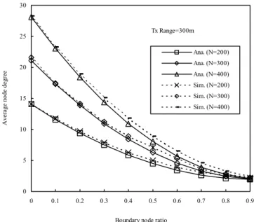
Tx Range=300m 0 5 10 15 20 25 30 0 0.1 0.2 0.3 0.4 0.5 0.6 0.7 0.8 0.9 Boundary node ratio
Average node degree
Ana. (N=200) Ana. (N=300) Ana. (N=400) Sim. (N=200) Sim. (N=300) Sim. (N=400)
Figure 9 The average node degree approximates to 2(N-1)/N as the boundary node ratio increases.
any node v located at the vicinity of the border of Ainner, a
pseudo node in Aborder is regarded as neighbor of node v if they
are direct connected. With this modification, we repeat the simulation and the results are shown in Figure 7 and Figure 8. Apparently, after considering the border effect, we achieve a very good consistency between simulation and analyses. As mentioned in Section I, power consumption is an important concern in designing wireless ad hoc network. To minimize the power consumption, Figure 8 provides a way to select the optimum transmission range to construct a connected wireless ad hoc network. For example, if the transmission range is set to 300m, the constructed wireless ad hoc network is connected with very high probability. Figure 9 shows the impact of boundary node on the average node degree in an ( , )N B
connected wireless ad hoc network. In Figure 9, as stated in Theorem 3, under fixed transmission range 300m and different total number of nodes the average node degree decreases as the boundary node ratio increases. Besides, as the boundary node ratio approaches to unity, the average node degree asymptotically decreases to 2(N-1)/N. This result verifies
Theorem 3.
V. CONCLUSIONS
To provide an efficient topology control scheme, we first analyze the optimum transmission range to provide a power efficient connectedness control for wireless ad hoc networks. We first provide a probability upper bound for a wireless ad hoc network to have no isolated node. With the variation of the probability upper, one can achieve the conservation of power consumption by minimizing the transmission range while maintaining the required probability of connectivity. In addition, according to results in [7] and [8], this probability upper bound can also provides a criterion for a wireless ad hoc network to be connected. We also study the connectedness and
average node degree problems caused by the boundary node based on an ( , )N B wireless ad hoc network model. Based on this network model, the maximum number of boundary nodes that remains the network connectivity and the minimum average node degree of an ( , )N B connected wireless ad hoc network are derived.
REFERENCES
[1] Y. C. Cheng and T. G. Robertazzi, “Critical connectivity phenomena in multihop radio networks,” IEEE Trans. on Communications, vol. 37, no. 7, pp. 770-777, 1989.
[2] T. K. Philips, S. S. Panwar, and A. N. Tantawi, “Connectivity properties of a packet radio network model,” IEEE Trans. on Information Theory, vol. 35, no. 5, pp. 1044-1047, 1989.
[3] P. Piret, “On the connectivity of radio network,” IEEE Trans. on
Information Theory, vol.37, no. 5, pp. 1490-1492, 1991.
[4] P. Santi and D. M. Blough, “An evaluation of connectivity in mobile wireless ad hoc networks,” IEEE Proc. of the International Conference
on Dependable System and Networks (DSN’02), 2002.
[5] P. Gupta and P. R. Kumar, “Critical power for asymptotic connectivity in wireless networks,” in Stochastic Analysis, Control, Optimization and
Applications: A Volume in Honor of W. H. Fleming, W.M. McEneany,
G. Yin, and Q. Zhang, Eds. Boston, MA: Birkhauser, 1998, pp. 547– 566.
[6] P. Panchapakesan and D. Manjunath, “On the transmission range in dense ad hoc radio networks,” in Proc. SPCOMM 2001, Bangalore, India, July 2001, Paper 01-38.
[7] C. Bettstetter, “On the minimum node degree and connectivity of a wireless multihop network,” ACM MOBIHOC’02, pp. 80-91, 2002. [8] M. D. Penrose, “On k-connectivity for a geometric random graph,”
Wiley Random Structures and Algorithms, vol. 15, no. 2, pp. 145-164,
1999.
[9] D. B. West, Introduction to Graph Theory, Prentice Hall, 2001. [10] C. Bettstetter and O. Krause, “On border effects in modeling and
simulation of wireless ad hoc networks,” Proc. IEEE International
Conference on Mobile and Wireless Communication Networks (MWCN),