Electrophoretic Mobility of a Concentrated Suspension of Spherical Particles

Electrophoretic Mobility of a Concentrated Suspension

of Spherical Particles

Eric Lee, Jhih-Wei Chu, and Jyh-Ping Hsu1

Department of Chemical Engineering, National Taiwan University, Taipei, Taiwan 10617, Republic of China Received July 17, 1998; accepted September 23, 1998

The electrophoretic behavior of concentrated spherical colloidal particles is analyzed theoretically for all levels of scaled surface potentialf_a, taking the effect of double-layer polarization (DLP) into account. The result of numerical simulation reveals that for a very smallka (<0.01), k and a being, respectively, the reciprocal Debye length and the particle radius, or a very largeka (>100), using a linearized Poisson–Boltzmann equation (PBE) and ne-glecting the effect of DLP is reasonable; for an intermediateka, appreciable deviation may result. The deviation is negative ifka is small, and positive ifka is large. The mobility against ka curve may have a local minimum and a local maximum. Iff_ais low, the mobility increases with the porosity of the system under consid-eration, and for a fixed porosity, the mobility increases withka. If fais high andka is small, the effect of fa(i.e., solving a nonlinear

PBE) on the mobility of a particle is more significant than that of double-layer polarization, and the reverse is true ifka is large. For an intermediateka, the effect of DLP is more significant than that of fa when the porosity is high, and the reverse is true if it is

low. © 1999 Academic Press

Key Words: electrophoretic mobility; double-layer polarization,

concentrated suspension; spherical particles.

INTRODUCTION

Electrophoresis is one of the electrokinetic phenomena which has various applications in practice. Typical example includes separation of proteins and stabilization of soft soil. The phenomenon is governed by the so-called electrokinetic equations, which comprise the equation that describes the conservation of ions, the Poisson–Boltzmann equation, and the Navier–Stokes equation. The second describes the spatial vari-ation of the electrical potential, and the last the flow field of the system under consideration. In general, these equations are nonlinear and coupled with each other, which renders them extremely difficult to solve analytically. Often, it is assumed that the electrical potential is low and the electrical double layer around a charged entity is either very thick or very thin. Under these conditions, the Poisson–Boltzmann equation can be linearized and decoupled from the Navier–Stokes equation

(1– 4, 7–9). Otherwise, the electrokinetic equations needed to be solved numerically (5, 6). Previous investigations are fo-cused mainly on the behavior of an isolated particle in an infinite solution (1–9). In other words, the presence of other objects, such as the rigid boundary and nearby entities, is assumed to have a negligible influence on its behavior. By adopting a unit cell model, Levine and Neale (10) derived the electrophoretic mobility of a system containing multiple spheres under the condition of low electrical potential, which is valid for an arbitrary thickness of the double layer. They concluded that, due to the overlapping of the electrical double layers, the mobility decreases rapidly with the increase in the thickness of a double layer and/or the decrease in the porosity of the system. The same problem was also discussed by Kozak and Davis (11, 12) and by Ohshima (13). In the former, an arbitrary level of electrical potential was considered, taking the effect of double-layer polarization (DLP), the distortion of the double layer near a charged entity due to its relative motion with respect to the surrounding liquid medium as a response to the applied electric field, into account, but the overlapping of the double layers between two nearby particles was neglected. In the latter, an approximate expression for mobility was derived in which the complicated numerical integration in-volved in Levine and Neale (10) was avoided. The approxi-mate expression was found to have a relative error less than 4%.

In the present work, the electrophoresis of concentrated spherical colloidal particles is analyzed theoretically for all levels of electrical potential, taking the effect of DLP, which was neglected in most of the aforementioned studies, into account. In this case the general electrokinetic equations needed to be solved simultaneously. The idealized model adopted by Zydney (14) is used in conjunction with the pseu-do-spectral discretization scheme proposed in our previous study for the case of a sphere in a spherical cavity (15, 16).

THEORY

We consider identical, non-conducting, spherical particles of radius a in a z1:z2 electrolyte solution, z1 and z2 being,

respectively, the valences of cations and anions, and a 5

1_{To whom correspondence should be addressed. E-mail: t8504009@ccms.}

ntu.edu.tw.

240

0021-9797/99 $30.00

Copyright © 1999 by Academic Press All rights of reproduction in any form reserved.

2z2/z1. The electroneutrality in the bulk liquid phase requires

that n205 (n10/a), n10and n20being the bulk concentrations

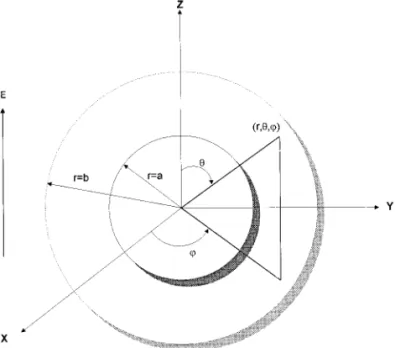
of cations and anions, respectively. The unit cell model pro-posed by Levine and Neale (10) is used. Referring to Fig. 1, each sphere is surrounded by a concentric spherical shell of liquid phase of radius b. The spherical coordinates (r,u, w), with origin at the center of the particle, are adopted in the following analysis. A uniform electric field E is applied in the

z-direction (u 5 0). Suppose that the liquid phase is

incom-pressible and has constant physical properties. Also, the motion of particles is slow so that the system under consideration is at a quasi-steady state. Under these conditions, the electro-phoretic motion of the particle is governed by the following set of three equations.

Conservation of Ions

The conservation of ions leads to

Y¹ z

F

F

kT Y¹f

G

G

where Y¹ denotes the gradient operator, e and f are, respec-tively, the elementary charge and the electrical potential, vY represents the fluid velocity, k and T are the Boltzmann constant and the absolute temperature, respectively, and nj, Dj,

and zj are the number concentration, the diffusivity, and the

valence of ion species j, respectively.

Electrical Potential

Here, we assume that the time scale for double-layer relax-ation is much smaller than that of the motion of a particle, and,

therefore, the spatial variation of the electrical potential can be described by the Poisson–Boltzmann equation

¹2_{f 5 2}r

e 5 2_j

O

zjenj

e , [2]

wheree and r denote the permittivity of the liquid phase and the spatial charge density, respectively.

Flow Field

The flow field is described by the Navier–Stokes equation in the creeping flow region

Y¹ z vY 5 0 [3]

h¹2

v

Y 2 Y¹p 2r Y¹f 5 0, [4]

where p,h, and r denote, respectively, the pressure, the vis-cosity, and the density of fluid.

Suppose thatf can be decomposed as (16)

f 5 f11f2, [5]

wheref1andf2represent, respectively, the electrical potential

that would exist in the absence of the applied electric field and that outside the particle arising from the applied electric field. The effect of DLP is taken into account by considering the expression (6)

nj5 nj0exp

S

zje~f11f21 gj!

kT

D

where gj denotes a perturbation function for potential which

accounts for the effects of fluid flow on concentration. Iff2

and gjare small compared to both kT/e andf1, Eq. [6] can be

linearized as nj5 nj 0exp

S

DF

G

particle is characterized by the zeta potentialza. It should be

pointed out that the fact thatf2and gjare small does not imply

that their effects are insignificant (6).

For convenience, scaled properties are used in the following analyses. Here, the radius of a particle a is chosen as the characteristic length and the electrophoretic velocity of an isolated particle in an electric field of strength (za/a) based on

the Smoluchowski’s theory UE(5eza

2

/ha) as the characteris-tic velocity. Instead of solving Eqs. [3] and [4] directly for FIG. 1. Schematic representation of the system under consideration.

velocity and pressure, the governing equation which describes the stream function c, obtained by taking the curl of Eq. [4] subject to Eq. [6], is solved. The r- and u-components of velocity v, vr, and vu, can be evaluated from c by vr 5

2(­c/­u )/r2

sinu and v_u5 (­c/­r)/r sin u, respectively. For convenience, a scaled stream potential c* 5 c/UEa

2

is de-fined.

The symmetric nature of the spherical coordinates adopted suggests that the problem under consideration can be reduced to a one-dimensional one (16); i.e.,f*2, g*1, g*2, andc* can be

written as f*2 5 F2(r)cos u, g*1 5 G1(r)cos u, g*2 5

G2(r)cosu, and c* 5 C(r)sin

2_{u. The governing equations,}

Eqs. [1]–[4], are then simplified under the above statements. It can be shown that the variation of f*1, the scaled electric

potential at equilibrium, is governed by

Lf*15 2 1 ~1 1a! ~ka!2 fr @exp(2f rf*1! 2 exp(afrf*1)], [8]

where the scaled surface potentialfr, the operator L, and the

Debye–Huckel parameterk are defined, respectively, by

fr5zaz1e/kT [8a] L; d 2 dr*21 2 r* d dr*2 2 r*2, [8b]

where r* 5 r/a, and

k 5

F

O

G

The boundary conditions associated with Eq. [8] are

f*15 1 at r* 5 1 [8d]

df*1

dr* 5 0 at r* 5 b/a, [8e]

where the second condition implies that the unit cell as a whole is electrically neutral, and there is no current flow between adjacent cells. Equation [8] needs to be solved simultaneously with the equations (16)

F

2

11a @exp~2frf*1! 1a exp~afrf*1!#

G

5 ~ka!

2

11a @G1exp~2frf*1! 1aG2exp~afrf*1!# [9]

LG12fr df*1 dr* dG1 dr*5 Pe1v*r df*1 dr* [10] LG21afr df*1 dr* dG2 dr*5 Pe2v*r df*1 dr* [11] D4_{C 5 2} ~ka! 2 11a

F

G

where Pej 5 e(Z1e/kT)2/hDj, j 5 1, 2, is the electric Peclet

number of ion species j, n*1 5 exp(2frf*1), n*2 5

exp(afrf*1), and the operator D4is defined as

D4_{5 ~D}2_!2₅

S

D

The boundary conditions associated with Eqs. [9]–[12] are

dF2 dr*5 0 at r* 5 1 [13a] dF2 dr*5 2E*z at r*5 b/a [13b] dGj dr*5 0 at r* 5 1, j 5 1, 2 [13c] Gj5 2F2 at r*5 b/a, j 5 1, 2 [13d] C 5 21₂U*r*2 and dC dr*5 2U*r* at r* 5 1 [13e] C 5

F

G

where E*z 5 Eza/za, and U* 5 U/UE, Ez and U being,

respectively, the z-component of the electric field and the terminal velocity of a particle. In these expressions, Eq. [13a] states that the particle is non-conducting, Eq. [13b] specifies the applied electric field, Eq. [13c] implies that the particle surface is impermeable to fluid, Eq. [13d] suggests that ion species achieve the equilibrium value at the virtual surface, and Eq. [13e] states that the particle is moving with velocity U. Equation [13f] implies that the virtual surface is steady and satisfies Kuwabara’s model of zero vorticity; this will lead to a result which is consistent with that predicted by the Smoluchowski’s equation for the case of isolated particles (10).

The mobility of a particle can be evaluated on the basis of a force balance. At the steady state, the sum of the external forces acting on a particle in the z-direction, which includes the electrical force FEzand the hydrodynamic force FDz, vanishes.

FEz5 8 3peza 2

S

D

S

S

DD

According to O’Brien and White (6), the problem of solving Eqs. [8]–[13f] can be decomposed into two sub-problems. In the first problem a particle moves at a uniform velocity U in the absence of the applied field, and in the second problem, the particle is held fixed in the applied electric field. The force required to move the particle in the first problem, f1, can be

expressed as f15dU*, and the force exerts on the particle in

the second problem, f2, as f25 bE*z. Therefore, we have U*m

5 U*/E*z 5 2b/d, U*m being the scaled mobility of the

particle. Here,d denotes the force per unit velocity exerting on a particle in the absence of electric field, and2b is the sum of the scaled electric force in the z-direction, F*Ez(5FEz/peza

2

), and the scaled drag force in the z-direction, F*Dz(5FDz/peza

2

). Details about the derivations of the governing equations, cal-culation of mobility, and the numerical scheme employed can be found in Lee et al. (16).

RESULTS AND DISCUSSION

Figure 2 shows the variation of the scaled mobility U*mas

a function ofka at various levels of scaled surface potential

fafor the case in which the effect of DLP is neglected. The

result of Ohshima (13), which was based on a linearized Poisson–Boltzmann equation (LPBE) and which neglected the effect of DLP, is also presented for comparison. For convenience, Ohshima’s model is abbreviated hereafter as

OM. As can be seen from Fig. 2, U*m increases

monotoni-cally with ka. For fixed particle size, this implies that the thicker the electrical double layer (smallerk), or the more significant the electrical interaction between two particles, the smaller the mobility. This is consistent with the predic-tions of Levine and Neale (10). Figure 2 suggests that if DLP is neglected, using LPBE will underestimate the mo-bility, in general. The deviation becomes insignificant, how-ever, ifka is either very small or very large. A comparison of the present result with that of OM reveals that the effects of DLP and relaxation are reflected by the terms involving

ka in Eqs. [9] and [12]. If ka is small, it reduces to the

corresponding expression of OM, and the effect of DLP becomes negligible.

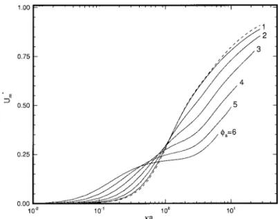
The variations of the scaled mobility U*mas a function ofka

at various levels of scaled surface potentialfafor the case in

which the effect of DLP is taken into account are illustrated in Figs. 3 and 4 for two different H (5a/b). The result based on OM is also presented in these figures for comparison. Here, due to the nature of the pseudo-spectral method adopted, the nu-merical procedure becomes inefficient ifka exceeds a critical value, which depends largely on the magnitudes of H andfr.

Nevertheless, the general trend can still be predicted. Figures 3 and 4 reveal that, for a very small (,0.01) or a very large (.100) ka, OM is satisfactory. For an intermediate ka, de-pending upon the magnitudes of ka, H, and fa, OM may

either underestimate or overestimate U*m. The deviation

de-pends largely upon two competing factors. First, as pointed out previously, using LPBE will underestimate U*m. Second,

ac-cording to Kozak and Davis (11, 12), the electric field induced by a charged particle has the effect of lowering the applied electric field, and therefore, using LPBE will overestimate U*m.

Note that, since double-layer interactionis neglected in their analysis, the conclusion is suited for largeka only. Also, for

FIG. 3. Variation of scaled mobility U*m as a function ofka at various

levels of scaled surface potentialfafor the case Pe15 Pe25 0.1 anda 5 1. Key: same as Fig. 2.

FIG. 2. Variation of scaled mobility U*m as a function ofka at various

levels of scaled surface potentialfa. Key: H5 0.5; a 5 1; b 5 2; (---) result

fixed surface potential, the thinner the electrical double layer (largerka), the greater the gradient of potential, and, therefore, the stronger the electric field induced by a particle. On the other hand, referring to Fig. 2, the first factor is more pro-nounced for a smaller ka. Therefore OM will underestimate

U*mifka is small, and it will overestimate U*mifka is large.

Note that according to Fig. 2, in the absence of the effect of DLP U*m increases with ka. On the other hand, if DLP is

considered, since the electric field induced by a charged par-ticle has the effect of lowering the applied electric field, the larger theka, the stronger the electric field induced, and there-fore, the smaller the U*m. The net effect is that the variation of U*mas a function ofka may have a local minimum and a local

maximum, as can be seen from Fig. 4. A comparison between Figs. 3 and 4 reveals that if H is large, or the concentration of particles is high, the local extreme can be observed at a lower surface potential.

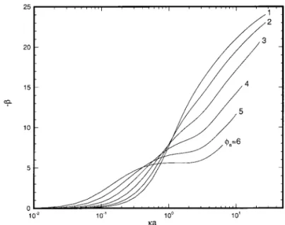
Figures 5 and 6 show, respectively, the variations of the scaled electric force in the z-direction F*Ez and the parameter 2b as a function of ka at various levels of scaled surface

potential fa. Figures 3, 5, and 6 reveal that the variations of U*mand F*Ezhave the same trend. Since U*m5 2b/d and 2b

5 F*Ez 1 F*Dz, the qualitative behavior of U*m is mainly

determined by2b, and d has a quantitative effect on U*monly.

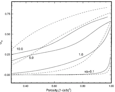
This is similar to the case of a particle in a cavity (16). The variations of the scaled mobility U*mas a function of the

porosity of the system under consideration, defined by [1 2 (a/b)3], at various values of ka for two levels of surface potentialfaare illustrated in Figs. 7 and 8. The corresponding

results predicted by OM are also shown for comparison. Note that if the porosity becomes unity, the system reduces to isolated particles. Figure 7 suggests that if fa is low, U*m

increases with porosity, and for a fixed porosity, U*mincreases

with ka. The deviation of OM from the present model is

inappreciable. As suggested by Fig. 8, however, it becomes significant at a higherfa. In this case, ifka is small (,0.1),

the effect offa(i.e., solving a nonlinear Poisson–Boltzmann

equation) on the mobility of a particle is more significant than that of DLP, and OM will underestimate U*m. On the other

hand, ifka is large (.10), the reverse is true. For an interme-diateka, the effect of DLP is more significant than that of fa

when the porosity is high, and the reverse is true if it is low. The variations of the scaled mobility U*mas a function ofka

at various values of a (5 2z2/z1 5 2valence of anions/

valence of cations) are shown in Figs. 9 and 10. Since n*25

exp(afrf*1), the extent of the variation of n*2as the electrical

potential changes varies witha. If a . 1, increasing a has the effect of raising the absolute value of the second term in the FIG. 4. Variation of scaled mobility U*m as a function ofka at various

levels of scaled surface potentialfafor the case Pe15 Pe25 0.1 anda 5 1. Key: same as Fig. 2 except that H5 0.833.

FIG. 5. Variation of scaled force F*Ezas a function ofka at various levels of scaled surface potentialsfafor the case Pe15 Pe25 0.1,a 5 1, H 5 0.5,

a5 1, and b 5 2.

FIG. 6. Variation of parameter2b as a function of ka at various levels of scaled surface potentialsfafor the case in Fig. 5.

square bracket on the right-hand side of Eq. [7]. This is similar to the effect of increasingfr. A comparison between Figs. 3

and 9 reveals that the effect ofa on the qualitative behavior of the U*magainstka curve is similar to that of fa. Conclusions

similar to those obtained from Fig. 9 can be drawn from Fig. 10 for the case in whicha , 1.

The major difference between the present work and the relevant studies in the literature can be summarized as follows. In the analysis of Levine and Neale (10) the linearized Pois-son–Boltzmann equation, i.e., the linearized version of Eq. [8], was considered. The effects of DLP and relaxation were ne-glected, but the overlapping of adjacent double layers was

taking into account. That is, the right-hand side of Eq. [9] was assumed to be zero, and the boundary condition, Eq. [8e], was adopted. The effect of DLP was considered by Kozak and Davis (11). However, since the equilibrium potential within a cell was approximated by that of an isolated particle, Eq. [8e] was not considered, and therefore, the result obtained is best suited for the case of thin double layers; i.e., the interaction between adjacent double layers is insignificant. The analysis of Ohshima (13) is similar to that of Levine and Neale (10). The main difference between the two is that the former proposes an approximate method which is capable of simplifying the com-plicated exact solution of the latter.

FIG. 7. Variation of scaled mobility U*m as a function of porosity at

various values ofka for the case Pe15 Pe25 0.1,fa5 1, anda 5 1. Key:

(---) result of Ohshima (13).

FIG. 8. Variation of scaled mobility U*m as a function of porosity at

various values ofka for the case Pe15 Pe25 0.1,fa5 3, anda 5 1. Key:

same as Fig. 7.

FIG. 9. Variation of scaled mobility U*m as a function ofka at various

values ofa (5 2valence of anions/valence of cations) for the case Pe15 Pe2 5 0.1 andfa5 1. Key: same as Fig. 2.

FIG. 10. Variation of scaled mobility U*mas a function ofka at various

ACKNOWLEDGMENT

This work is supported by the National Science Council of the Republic of China. REFERENCES

1. Von Smoluchowski, M., Z. Phys. Chem. 92, 129 (1918). 2. Huckel, E., Phys. Z. 25, 204 (1924).

3. Henry, D. C., Proc. R. Soc. London Ser. A 133, 106 (1931). 4. Booth, F., Proc. R. Soc. London Ser. A 203, 514 (1950).

5. Wiersema, P. H., Loeb, A. L., and Overbeek, J. Th. G., J. Colloid Interface Sci. 22, 78 (1966).

6. O’Brien, R. W., and White, L. R., J. Chem. Soc. Faraday Trans. 2 74, 1607 (1978).

7. O’Brien, R. W., and Hunter, R. J., Can. J. Chem. 59, 1878 (1981).

8. Ohshima, H., Healy, T. W., and White, L. R., J. Chem. Soc. Faraday Trans. 2 79, 1613 (1983).

9. Ohshima, H., Adv. Colloid Interface Sci. 62, 189 (1995).

10. Levine, S., and Neale, G. H., J. Colloid Interface Sci. 47, 520 (1974). 11. Kozak, M. W., and Davis, E. J., J. Colloid Interface Sci. 127, 497

(1989).

12. Kozak, M. W., and Davis, E. J., J. Colloid Interface Sci. 129, 166 (1989).

13. Ohshima, H., J. Colloid Interface Sci. 188, 481 (1997). 14. Zydney, A. L., J. Colloid Interface Sci. 169, 476 (1995).

15. Lee, E., Chu, J. W., and Hsu, J. P., J. Colloid Interface Sci. 196, 316 (1997).

16. Lee, E., Chu, J. W., and Hsu, J. P., J. Colloid Interface Sci. 205, 65 (1998).