發光二極體於功能性頻譜照明之研究

國立交通大學

光電工程研究所

博士論文

發光二極體於功能性頻譜照明之研究

An investigation into functional spectral illumination

with LED white composite spectra

研究生：簡銘進

指導教授：田仲豪教授

發光二極體於功能性頻譜照明之研究

An investigation into functional spectral illumination

with LED white composite spectra

研

究 生：簡銘進

Student : Ming-Chin Chien

指導教授：田仲豪

Advisor : Dr. Chung-Hao Tien

國立交通大學 電機學院

光電工程研究所

博士論文

A Thesis

Submitted to Institute of Electro-Optical Engineering

College of Electrical Engineering and Computer Science

National Chiao-Tung University

in Partial Fulfillment of the Requirements

for the Degree of Doctor of Philosophy

in

Electro-Optical Engineering

July 2012

Hsin-Chu, Taiwan, Republic of China

發光二極體於功能性頻譜照明之研究

博士研究生：簡銘進 指導教授：田仲豪教授

國立交通大學

光電工程研究所

摘 要

隨著近年發光二極體(Light emitting diode, LED)的快速發展，多種 LED 頻譜組合 的 LED 系統已充分具有應用潛能，可根據不同操作目的策略性的調制其複合頻 譜能量分布。以一般照明為例，對於一目標色溫，LED 系統可藉由頻譜調制提 升整體效率與演色性，並拓展適用的環境溫度範圍。延伸到智能照明，則可根據 使用者對照明色溫變化的需求調整到對應的頻譜，同時維持系統高效能運作。在 醫療照明上的應用，需要更著重於頻譜在溫度與電流變化下的可預測性。 然而，一般而言高功率單色光或螢光轉換的 LED，其 SPD 的變化相對於接 面溫度與驅動電流為非線性的關係，因而增加了系統頻譜優化的困難度，導致上 述的應用目標難以達成。本論文基於目前市面上商用的 LED 元件，以現有的製 程與材料為基礎，針對各終端應用發展一種 LED 頻譜調制最佳化的解決方案， 建立精確頻譜模型與完整的優化設計流程。 本論文提出將一般非完全對稱的 LED 頻譜分解成雙高斯函數，準確的預測 LED 頻譜在不同溫度與電流下的行為，並將此模型推展到螢光粉轉換白光 LED (phosphor-converted white LED)。

本論文並嘗試以不同角度切入，成功引入透鏡幾何光學系統設計的概念，針 對複合 LED 照明系統 SPD 提出相對應的完整設計流程: (1) 初始系統, (2) 邊界 條件, (3) 優化, (4) 價值函數分析, (5) 判斷, 與 (6) 容忍度分析。最終以此技術 分別應用於低功率與高功率 LED 照明系統，實現色溫可調、適用環境溫度廣泛、 演色性佳的高效率照明設計。

An investigation into functional spectral

illumination with LED white composite spectra

Doctoral Student: Ming-Chin Chien Advisor: Dr. Chung-Hao Tien

Institute of Electro-Optical Engineering National Chiao Tung University

Abstract

With the rapid progress in light-emitting diode techniques, all kinds of lighting purposes can be achieved by strategically manipulating the spectral power distributions of LEDs clusters. For example, in general lighting there is a fundamental tradeoff between the efficiency and color rendering quality, where an optimal boundary (the Pareto Front) will be produced. By optimizing the composite spectrum, the LEDs lighting system can be operated alongside the boundary. When the spectral-controllable technique is utilized to fields of intelligent illumination, the color temperature can be adjusted in accordance with end demands. As to the medical lighting, the spectral distortion will be predictable with respect to variant ambient temperature and drive current.

In this dissertation, a novel methodology for spectral manipulation has been proposed, including a well-defined spectral model and six optimization steps. The spectral model employing the double-Gaussian function can closely estimate the practical spectrum that is imperfectly symmetric and depends on the junction temperature. For the optimization, the concept in imaging system design has successfully been adopted to develop a composite spectral process. The proposed

achieve the color-turntable systems with high efficiency, high color rendering property as well as wide operation window at ambient temperature.

誌 謝

一轉眼，加入田仲豪老師的研究群已經八年了。一路走來，有許多的點滴在 心頭；在這些年的研究當中，要感謝的人真的很多，僅以此文表達我的誠摯謝意。 我衷心的感謝田仲豪老師在研究上、表達能力上、甚至生活細節上的悉心指 導，並提供十分優良的研究環境，讓我有許多的機會到國內外的企業或是研究單 位實習，並參加國際級的研討會以開闊我的視野。也由衷的感謝Stefan Sinzinger 教授在Ilmenau半年的細心照顧與指導，且在我回國後更仍不斷的關心與鼓勵 我。能成為田老師與Sinzinger教授的指導學生，實在是我畢生的福氣且著實讓我 受益良多，因此方能順利地完成本篇論文。此外，也感謝各位口試委員所提供的 寶貴意見，使本論文更加的完備。 在這些年的研究生活中，要感謝李企桓學長、鄭裕國學長、鄭榮安學長與鄭 璧如學姊對我的引領與幫忙，也感謝一同奮鬥的小陸、健翔與Blue，和你們一起 的相互討論與扶持，是研究生活裡很大的助益。另外，這些年來一同工作過的學 弟妹們，貢丸、松柏、董哥、志宏、玉麟、及筱儒，謝謝你們的協助，也給了我 許多與你們一同學習的機會。而對於許多已經畢業的優秀碩士班學弟妹們，以及 目前在這個實驗室繼續奮鬥的同儕們，謝謝你們一同經營了這個溫馨且愉快的研 究環境，還要謝謝最照顧我的助理古明嬿小姐以及其他美麗的助理小姐們，讓我 八年來的研究生活充滿了無限的回憶。

在Technische Universität Ilmenau研究的期間，感謝Matthias、Jürgen、Karolin、

馬玄與欣育的照顧，讓我少吃很多的苦頭，也謝謝Sinzinger教授實驗室其他幫忙 我的好朋友們，讓我在德國半年期間度過了非常美好的時光。 此外，在沛鑫半導體實習的日子，要感謝陳志隆教授與韋安琪學姊的指導， 使我對於光學設計在實作上有更進一步的認識，也感謝玉樹、育佳及小小，還有 許多曾經幫助過我的人，謝謝你們的協助。 對於我最親愛的父母親，真的謝謝你們三十年來對我的支持與鼓勵，讓我變 得更有自信且成熟穩重，如今我即將邁入人生的另一個階段，在未來的日子裡我 必當竭盡所能來報答你們、孝順你們。而在這些日子裡，真的很感謝陪伴著我的 筱儒，在我最低潮的時候有妳陪我一起渡過，最開心的時候有妳跟我一起分享；

Contents

Abstract (Chinese) ………i

Abstract (English) ………...ii

Contents ………….………..v

List of Figures ………….………..viii

List of Tables ……….…….……….xi

List of Symbols ………….…….……….xii

1 Introduction ... 1

1.1 Additive mixing ... 2

1.1.1 Simplified mixing condition ... 2

1.1.2 Ideal trichromatic color mixing scheme ... 4

1.2 Thermal and current dependences of LEDs spectra ... 7

1.2.1 Prior arts in consideration of thermal and current issues ... 8

1.3 Ideal multispectral mixing optimization ... 9

1.4 Aspects regarding the practical realization of LEDs cluster ... 11

1.4.1 Spectral characteristic ... 11

1.4.2 Color quality index ... 11

1.4.3 Energy evaluation ... 12

1.5 Motivation and objective of this thesis ... 12

1.6 Organization of this thesis ... 14

2 LED Spectral Characterization ... 16

2.0 Goal ... 16

2.1 Junction temperature measurement ... 17

2.1.1 Forward voltage method ... 17

2.1.2 Junction temperature estimation ... 18

2.2 Junction temperature determination ... 22

2.3 LED spectral modeling ... 25

2.3.1 Double Gaussian model ... 25

2.3.3 Phosphor-converted spectral function ... 29

2.4 Validation of the spectral model ... 30

2.5 Summary and conclusions ... 32

3 Multispectral Mixing Optimization as Lens Design Techniques

... 34

3.0 Goal ... 34

3.1 Initial system ... 36

3.2 Define boundary conditions ... 38

3.3 Optimization ... 39

3.3.1 Metamerism ... 39

3.3.2 Continous genetic alogrithm ... 42

3.4 Merit analysis ... 45

3.4.1 Merit function and Pareto front ... 45

3.4.2 Sampling method SA1 ... 46

3.4.3 Sampling method SA2 ... 48

3.5 Judgment ... 49

3.6 Tolerance analysis ... 50

3.7 Summary and conclusions ... 51

4 Applications of the Multispectral Mixing Scheme ... 52

4.0 Goal ... 52

4.1 Case 1: Low power LEDs cluster design ... 53

4.1.1 Validation of the composite spectrum ... 54

4.1.2 Comparison of R/G/B and R/G/B/A system ... 55

4.1.3 The effect of cool-white LED ... 57

4.1.4 The color tunable R/G/B/A/CW system ... 59

4.2 Case 2: High power LEDs cluster design ... 59

4.2.1 The influence of ambient temperature on color mixing... 60

4.2.2 Spectral modulation with thermal compensation ... 62

4.2.3 Optimized pentachromatic LEDs cluster ... 65

5 Conclusions and Future Works ... 68

5.1 Conclusions ... 68

5.1.1 LED Spectral Characterization ... 68

5.1.2 Multispectral Optimization as Lens Design Techniques ... 69

5.1.3 Applications of the Multispectral Mixing Scheme ... 70

5.2 Future works ... 71

5.2.1 Other applications ... 71

5.2.2 Reverse model ... 73

5.2.3 Summary ... 76

Appendix − Color rendering index and color quality scale……....…77

References and links………...………..…...80

Publication List ………..………....84

List of Figures

1-1. The schematic interaction between light sources, objects, and detectors ... 2 1-2. CIE 1931 and CIE 1978 x y z color matching functions. The CIE 1931 version

is the currently valid official standard [3]……….. 3

1-3. Principle of color mixing illustrated by three emission lines with chromaticity coordinates (x1, y1), (x2, y2), and (x3, y3). The mixed color has the coordinate (x, y)

... 6 1-4. The spectrum of phosphor-converted white LED changes with respect to ambient tmeperature Ta ... 7

1-5. Conceptual analogy between the SPD synthesis and conventional lens design. A LED cluster composed of red/cool-white/cool-white/green (R/CW/CW/G) can be regarded as adouble Gauss lens system with two singlet lenses and two cemented doublets, where the cool-whiteLED is caused by dichromatic mixing ... 14 2-1. Typical semi-log current-voltage characteristic of a green InGaN LED (HELIO

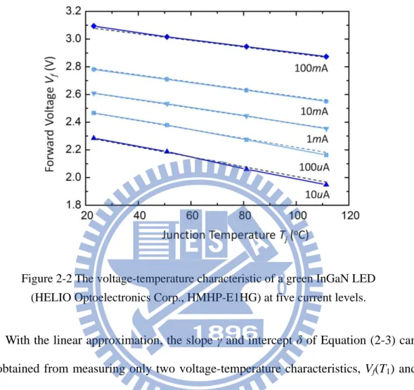
Optoelectronics Corp., HMHP-E1HG) ... 19 2-2. The voltage-temperature characteristic of a green InGaN LED (HELIO

Optoelectronics Corp., HMHP-E1HG) at five current levels ... 20 2-3. The distribution of all elements in Gaussian power p and its fitting coefficient

values cp1, cp2 and cp3 for the red AlInGaP LED ... 28

2-4. The deviation and goodness of fit for Gaussian power distribution fitting For the

red AlInGaP LED ... 28 2-5. The illustration of the simulation model and the experimental measurement for

green and phosphor LED spectra at Tj = 25 oC and IDC = 350 mA, respectively

... 30 3-1. Design procedure of (a) lens design and (b) spectral synthesis of a LED cluster.

Both flow charts include six steps: (3.1) initial system, (3.2) define boundary condition, (3.3) optimization, (3.4) aberration or merit analysis, (3.5) judgment,

3-2. Normalized luminous efficiency of visible LED made from GaInN and AlGaInP series versus individual peak wavelength. The LED with high LE is analogous to the lens with high refractive index ... 36 3-3. Schematic process of the continuous genetic algorithm (CGA) ... 42 3-4. (a) The illustration of the Pareto fronts PFs for different CTs on the CQS − LE

plane. (b) The flowchart of SA1. Either end point P0 or P1 located within quadrant

III will lead to an unacceptable performance as PF3. The curve with end points

located within quadrant II and IV, like PF2, should be confirmed the operation

portion (red curve) ... 47 3-5. A green wavelength inserted at the large wavelength interval ... 49 3-6. Two or more single-colour spectrum replaced by a phosphor- converted source

... 49 3-7. An operating wavelength of too-high emission split into two adjacent wavelength

... 50 4-1. The spectra of red (R), green (G), blue (B), amber (A) and cool-white (CW) LEDs

at ambient temperature Ta of 25 oC with all drive currents of 20 mA. The

corresponded chromaticity points and specifications are also shown in the figure. The drive currents controlled by PWM approach have the pulse width of 6.66 ms at differences of 0.04 ~ 0.06 ms for each gray level (a total of 128 gray levels) ... 53 4-2. Spectral comparisons of simulations and experiments for P0 and P1 at CTs of

6500K and 3000K, respectively. The simulated spectra closely matched the measurements in spite of a few peak deviations ... 54 4-3. The illuminant environments at (a) P0 (CQS = 87 points, LE = 66 lm/watt) for CT

= 6500K and (b) P0 (CQS = 69 points, LE = 67 lm/watt) for CT = 3000K show

apparently different color rendering abilities ... 55 4-4. The SA2 results of (a) R/G/B (black curve), R/G/B/A, and (b) R/G/B/A/CW

clusters aimed to P1 and P0 for full range of CT from 1000K to 10000K ... 56

SA2 analysis, R/G/B/A/CW can further extend the operation window in color

temperature ... 57

4-6. (a) The values of CQS and LE, and (b) the stacked emission power ratio versus color temperature for the optimized R/G/B/A/CW design (CQSm = 80 points and LEm = 60 lm/watt). The operation window has been extended to 2600K < CT < 8500K with the selected weight via SA2 selection method. It is noted that the operation window is mainly restricted by the CQS due to the correction factor at the extreme color temperature ... 58

4-7. The power spectra of red (λR: 625nm, ΔλR: 20nm), green (λG: 523nm, ΔλG: 33nm), blue (λB: 465nm, ΔλB: 25nm), amber (λA: 587nm, ΔλA: 18nm) and cool-white LEDs at Ta of 10 oC with IDC of 350 mA. The upper right figure shows a real-field test designed for CT = 5000K and the lower right one shows the utilized LEDs attached on the temperature controllable fixture respectively ... 60

4-8. The temperature dependence of spectra designed for CT = 3200K, 4600K, 6200K, and 7400K at Ta = 50 oC. The chromaticity point shifts toward higher color temperature with the raise of Ta owing to the dramatic deterioration in LEs of the red and amber LEDs ... 61

4-9. The temperature dependence of LE for pentachromatic LEDs. When Ta is varied from 10 oC to 100 oC, LEs of amber and red AlInGaP LEDs decrease to 23% and 46% of that at 10 oC while LEs of InGaP LEDs are insensitive to temperature variation ... 62

4-10. The LE contour of the pentachromatic LEDs cluster is performed under the predefined requirements (CQS> 85 points, lighting level =100 lm and Δxy < 0.01). When the LE = 100 lm/watt is selected as the minimum efficiency boundary, a full operation range for ambient temperature can be obtained for CT > 5200K ... 66

5-1. Configuration of the spectral tunable system ... 73

5-2. The schematic process of the reverse model ... 74

List of Tables

2-1. Pentachromatic LEDs, specific pulsed current I0 , slopes γ and γ’, and intercepts γ

and γ’ of the linear

approximation.……….………21

2-2. The values of fitting parameters c, d, e, and f for pentachromatic LEDs at ambient

temperature Ta = 50 oC………..………..24

2-3. The DC drive current IDC, electrical power Pe, optical power Φ and junction

temperature Tj for red AlInGaP LED (HELIO Optoelectronics Corp.,

HMHP-E1HR) at ambient temperature Ta = 50 oC………..24

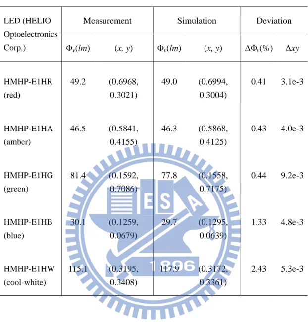
2-4. The parameters of approximated phosphor-converted LED spectrum. The blue and fluorescence components should be individually considered………..31 2-5. The comparison of the simulation and measurement on luminous flux and CIE

colour coordinates for all sample LEDs………..32 4-1. The comparison of CQS, LE, output spectral power P, correlated color

temperature CCT, color temperature CT and the input power ratio Pin under Ta =

10oC, 50oC and 100oC………...………..63

List of Symbols

The table below lists the symbols that were used in this thesis for quick reference. In some cases, the use of the same symbol to refer to two different things was inevitable. In such cases, the meaning should be clear from the context

A eigenvalue matrix

 random number within interval [0, 1]

B Boltzmann constant

c _{coefficients, the corresponded weight of point Pc}

c _{coefficient vector}

C coefficient matrix

C

C matrix of chromaticity coordinates

M

C matrix of color-matching functions

Cov covariance matrix

ˆ

M

C matrix of color-matching functions with values on peak wavelengths

 intercept

 small difference

e _{elementary charge}

E eigenvector matrix

E’ eigenvector matrix with the reduced dimentionality

f focal length

 _slope

g _{Gaussian function}

g _{Gaussian function vector}

G value of merit function

G Gaussian function matrix

I current p I pulsed current S I saturation current qu

i quadratic current basis vector

DC

i DC drive current vector

DC

i magnified DC drive current vector

DCP

I matrix of initial DC current population

K total types of LED

 wavelength

ˆ

ˆλ peak wavelength vector



 spectral width

Δλ spectral width vector

m _{number of spectral vector}

m basis vector

C

m vector of mixed light’s chromaticity coordinates

M total number of spectral vector

M basis matrix

n _{refractive index, number of sampling wavelength, number of population}

ideal

n ideality factor

N total number of sampling wavelength

O matrix operator

 optical lens power

 radiant flux

v

 luminous flux

p _{power of Gaussian function}

p _{Gaussian power vector}

e

P electric power

in

P electric power ratio

P principal component

r surface curvature

R radius of the lens surface

t

R thermal resistance between junction and reference point

s _{spectral function vector}

s vector of estimated spectral function

S spectral function

m

S mean value of the spectral function

S estimated spectral function

m

S mean value of the estimated spectral function

S spectral function matrix

S matrix of estimated spectral function

p

S matrix of estimated spectral population

t vector of target tristimulus values

t vector of current tristimulus values

j

t junction temperature vector

a

T ambient temperature

j

T junction temperature

jp

T matrix of junction temperature population

V photopic eye sensitivity function

DC V DC forward voltage f V forward voltage w _weight w _{weight vector} x _{chromaticity coordinate}

x color matching function of CIE 1931 x y z

X CIE 1931 XYZ tristimulus value

y _{chromaticity coordinate}

y color matching function of CIE 1931 x y z

Y CIE 1931 XYZ tristimulus value

z color matching function of CIE 1931 x y z

Chapter 1

Introduction

The progress in Light-emitting diodes (LEDs) technology has been breathtaking during the last few decades. At this time, great technological advances in LEDs are profoundly changing the way light was generated. In contrast to many conventional light sources, LEDs not only have the potential of converting electricity to light with near-unit efficiency, but also offer impressive controllability of their spatial distribution, temporal modulation, and polarization property . With an arrangement of multispectral LEDs, the LEDs cluster could particularly have the capability of manipulating its synthesized spectral power distributions (SPDs). Such intelligent light sources could be adjusted according to different operational environments and requirements. As a result, tremendous properties of LEDs or LEDs cluster lead to great benefits across a wide field of applications, including lighting, transportation, communication, imaging, agriculture, and medicine . In this doctoral research, we mainly focus on the spectral part of LEDs − in particular, spectral characterization and multispectral mixing methodology. A better understanding of additive mixing will be required to attain good design in practical applications.

1.1 Additive mixing

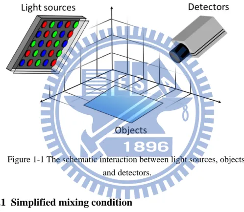
Figure 1-1 shows a general description of the additive mixing event. Light sources, e.g. LEDs clusters, are quantified by the spectral power distributions (SPDs). Objects are specified by the transmitted, reflected, or scattered spectral distributions, which depend on the illuminating and detecting geometrical conditions. The detectors are quantified through the sensor response curves.

Figure 1-1 The schematic interaction between light sources, objects, and detectors.

1.1.1 Simplified mixing condition

In order to elaborate the principle of additive mixing in a more understandable way, the condition is simplified by several assumptions:

1. Photometric units are used. The light and color sensation are characterized by the human eye. The luminance levels outside of the photopic vision regime and the spectral radiations beyond the human perceptual range are irrelevant when it comes to light perception by a human being. For example, when luminous level < 0.003 cd/m2 (scotopic vision regime), such as in a moonless night, objects lose

their colors but only appear to have different gray levels.

2. The influences of objects are eliminated. Objects are ideally regarded as white lambertian surfaces with unit spectral reflectance for all visible wavelengths. Thus the effects of the source-object-detector geometrical conditions on spectral detection are ignorable. The results of additive mixing only depend on the correlation of the synthesized spectral emissions and sensor response curves.

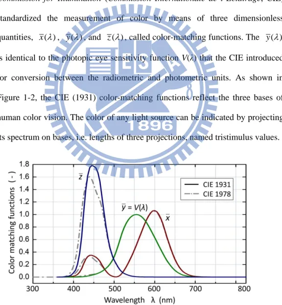
3. The sensor response curves are color-matching functions. The International

Commission for Illumination (Commission Internationale de l’Eclairage, CIE)

standardized the measurement of color by means of three dimensionless quantities, x( ) , y( ) , and z( ) , called color-matching functions. The y( ) is identical to the photopic eye sensitivity function V(λ) that the CIE introduced for conversion between the radiometric and photometric units. As shown in Figure 1-2, the CIE (1931) color-matching functions reflect the three bases of human color vision. The color of any light source can be indicated by projecting its spectrum on bases, i.e. lengths of three projections, named tristimulus values.

Figure 1-2 CIE 1931 and CIE 1978 x y z color matching functions. The

4. The number of multispectral light sources is three. Assume that the three emission bands have spectral distribution functoin S1(λ), S2(λ), and S3(λ), whose

bandwidths are much narrower than any of the color-matching functions. We further assume S1(λ), S2(λ), and S3(λ) have scalability and linearity with respect to

their drive currents. In addition, the chromaticity coordinates of three light sources (x1, y1), (x2, y2), and (x3, y3) are regularly located in the red, green, and

blue regions of the chromaticity diagram.

1.1.2 Ideal trichromatic color mixing scheme

Next, we determine tristimulus values X, Y, and Z of the mixed light from the aforementioned assumptions : 1 2 3 1 2 3 1 1 1 2 2 2 3 3 3 1 1 1 2 2 2 3 3 3 ( ) ( ) ( ) ( ) ( ) ( ) ˆ ˆ ˆ ˆ ˆ ˆ ( ) ( ) ( ) ( ) ( ) ( ) ˆ ˆ ˆ ( ) _DC ( ) _DC ( ) _DC X X X X x S d x S d x S d x S x S x S x c I x c I x c I                                 







(1-1) 1 2 3 ( )ˆ1 1 DC1 (ˆ2) 2 DC2 (ˆ3) 3 DC3 Y  Y Y Y  y  c I y  c I y  c I (1-2) 1 2 3 ( )ˆ1 1 DC1 (ˆ2) 2 DC2 (ˆ3) 3 DC3 Z Z Z Z  z  c I z  c I z  c I (1-3)

where Xi, Yi, and Zi are the tristimulus values of ith emission band. Similarly,ˆi and

IDCi refer to the peak wavelength and the DC drive current of the ith emission band

respectively. The factors c1, c2, and c3 are the constants, relating drive current IDC to

peak value of spectral function S( )ˆ for each light source. The Equations (1-1) − (1-3) can be expressed by a matrix form:

ˆ M DC C i = t (1-4a) 1 2 3 ₁ 1 2 3 2 3 1 2 3 ˆ ˆ ˆ ( ) ( ) ( ) ˆ _{( )}ˆ ₍ˆ _{) (}ˆ_{) , , and} ˆ ˆ ˆ ( ) ( ) ( ) M DC C i t DC DC DC x x x _{I X} y y y I Y I Z z z z    _           _{   }   _{   }    _{ } _{ }   _{   }         (1-4b)

Through this paper, vectors are denoted by bold-faced lower-case letters, e.g., t

(current tristimulus values), iDC (magnified DC drive current). Matrices are

represented by bold-faced capital letters, e.g., CˆM (peak values of color-matching functions). Equation (1-4) shows the system of trichromatic color mixing is critically determined, i.e. the system operator matrix CˆM is square. If we consider an inverse problem, the number of elements in the required vector t is equal to the number of components of the unknown vector iDC. In this case, solution of the inverse problem

is equivalent to finding a matrix operator O, which satisfies the condition:

DC

Ot = i (1-5) where the expression of t can be substituted by Equation (1-4) to yield the consequence:

ˆ -1 M

O = C (1-6)

The existence of inverse matrix ˆ 1 M

C  is based on the condition that row vectors of

system matrix CˆM are linearly independent. As a result, the DC drive current for each emission band is likely to be obtained.

To further gain the insight of additive color mixing, we calculate the set of chromaticity coordinates of the mixed light mC from the linear combination of

chromaticity coordinates of three light sources (x1, y1), (x2, y2), and (x3, y3): C C C w = m (1-7a) 1 3 1 2 2 1 2 3 3 , , and w x x x x w y y y y w     _{ }   _{ } _{ } _{ }     _{ }   C C C w m _(1-7b)

where the set of weight factors w is defined as:

1 _ˆ ( ) T M DC w = C i t sum (1-8)

Therefore, the principle of color mixing can be illustrated in Figure 1-3. Three chromaticity points, red, green, and blue, connected by the straight dash line, represent three vertexes of the triangle. The area of the triangle, called the color gamut, include all colors that can be linearly synthesized by the three emission bands.

Figure 1-3 Principle of color mixing illustrated by three emission lines with chromaticity coordinates (x1, y1), (x2, y 2), and (x 3, y 3). The mixed

For the case of dichromatic color mixing, w3 = 0, the color gamut will degenerate

to a straight line connecting two end points of two light sources, i.e. the edge of the triangle with end points red and green. Any chromaticity point locate on the line can be linearly combined by the two emission bands.

1.2 Thermal and current dependences of LEDs spectra

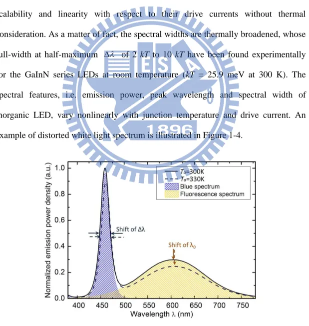
In previous section we have considered the narrower spectral widths of sources to simplify mixing mechanism. Furthermore, we assumed emission spectra have scalability and linearity with respect to their drive currents without thermal consideration. As a matter of fact, the spectral widths are thermally broadened, whose full-width at half-maximum  of 2 kT to 10 kT have been found experimentally for the GaInN series LEDs at room temperature (kT = 25.9 meV at 300 K). The spectral features, i.e. emission power, peak wavelength and spectral width of inorganic LED, vary nonlinearly with junction temperature and drive current. An example of distorted white light spectrum is illustrated in Figure 1-4.

Figure 1-4 The spectrum of phosphor-converted white LED changes with respect to ambient tmeperature Ta.

However, which raises the question as to the predictability and stability of LED-based light sources. Such spectral distortion therefore results in the drift of chromaticity point, color rendering property, and efficiency of the LEDs cluster . Taking a trichromatic mixing set of ˆ1= 455 nm (= 5.5 kT),ˆ2= 530 nm (=

7.9 kT), and ˆ3= 605 nm (= 2.5 kT) as an another example, which is designed for general lighting application. A slight shift of red peak wavelength from 605nm to 620nm will decrease the color rendering index CRI from 85 to 65 and the luminous efficacy of radiance LER from 320 lm/watt to 290 lm/watt, respectively. Similarly, a shift of green peak wavelength from 530 nm to 550 nm will decrease the CRI to the value less than 60, revealing that CRI is highly sensitive to the exact position of spectral peak .

The color rendering index CRI is a widely recognized figure of merit to evaluate the light quality of white light sources. Interested reader can refer to ref. [12] for more discussion about color appearance by various qualitative characteristics of lighting. The other figure of merit, the luminous efficacy of radiance LER, is defined as amount of luminous flux (lumen) converted from per unit optical power (watt).

1.2.1 Prior arts in consideration of thermal and current issues

In order to solve aforementioned issues, many efforts have been made to model the dependence of LED spectra on the temperature and current. In terms of theoretical interpretation, the LEDs emission spectrum is described by the product of the density of energy states within the allowed energy band and a Boltzmann energy distribution



. Most recently A. Keppens et al introduced this underlying physic into H. Y. Chou’s model, allowing for accurate simulations of single color LED spectra at any

quasi-physical model still needs to be empirically compensated.

In contrast to the physical consideration, mathematically using Gaussian function can simply incorporate the spectrum power distribution (SPD) with three spectral features . In 2005, a more general model on the basis of double Gaussian function was developed by Y. Ohno, which is nowadays still used by CIE . F. Reifegerste and J. Lienig, in 2008, evaluated the applicability of several mathematical functions for modeling of LED spectra; meanwhile, the formalism for low powered single-color LED in consideration of temperature and current was proposed . Nevertheless, a large number of fitting parameters precludes its transfer to practical use. Although many spectral radiant flux models have been published so far, to our knowledge, there is still lack of an easy-to-use modeling approach for high powered single-color LED, which is capable of simply extending to the spectrum modeling of phosphor- converted white light.

1.3 Ideal multispectral mixing optimization

In general, the mixing of multiple spectra based on LEDs can be accomplished by using (i) additive mixing of two or more single-color LED chips (LED-primary-based approach), (ii) wavelength-conversion via using phosphors or other materials (LED-plus-phosphor-based approach), and (iii) a hybrid approach composed of (i) and (ii) . In section 1.1, we have briefly discussed trichromatic mixing via LED- primary-based approach, where three emission sources for the trichromatic case are predetermined. Therefore, the linear system is critically determined. In fact, the selections of emission bands provide additional degrees of freedom, whose values will be highly relevant to the operational purposes. For example, a trichromatic combination of ˆ1 = 450 − 455 nm ( = 5 kT),ˆ2 = 525 − 535 nm ( = 5 kT),

and ˆ3 = 600 − 615 nm ( = 5 kT) is very favorable in terms of high color rendering lighting, resulting in a high CRI value in the range of 80−85 .

Now we generalize the condition by considering a synthesized SPD composed of

n undetermined emission bands, used for certain purpose with specific chromaticity

point. The problem is no longer critically determined but underdetermined, which is equivalent to subjecting the 2n-dimensional parameter space {ˆ1,…,ˆn,I1,…,In} to

three color-mixing constrains. In other words, an optimization happens in searching the best location, composed by two n-dimensional vectors { ˆ1 ,…, ˆn } and

{I1,…,In }, on the hypersurface with dimensionality 2n – 3. Where the best location

represents that composed spectrum provides the maximal benefit to the purposes. We could mathematically write the solution in a form as:

1 1

ˆ ˆ

arg max[{MF cons, } { , , _n, I,, I_n}] (1-8)

where MF is the merit function of the purposes. The term cons indicates three mixing constrains. In 2002, A. Žukauskasa et al. solved the above problem for general lighting applications . For simplicity, each emission band was assumed as a single Gaussian line with  = 6 kT. The optimal LEDs clusters for n = 2, 3, 4, and 5 were analyzed. Those results address the fundamental tradeoff between the luminous efficacy of radiance LER and the color rendering index CRI, which has the potential to provide a useful guide in the design of a polychromatic system.

1.4 Aspects regarding the practical realization of LEDs cluster

1.4.1 Spectral characteristic

To consider a practical system, first and foremost, more precise spectral characteristics should be imposed on sources instead of the artificial Gaussian distribution. In other words, the temperature and currents dependences of LEDs, as we mentioned in Section 1.2, should be predictable. In contrast to the ideal mixing condition, this additional temperature dependence results in the incensement of the dimensionality of the problem from 2n – 3 to 3n – 3. Eqation (1-8) would be rewritten as:

1 1 1

ˆ ˆ

arg max[{MF cons, } { , , _n, I ,, I_n, T,, T_n}] (1-9)

Such high dimensionality however raises the difficulty on searching the solution to satisfy Eqation (1-9). Therefore, crucial to this problem must be the dimensional reduction, e.g. using known types of sources. K. Man and I. Ashdown, in 2006, basically solved a mixing issue with three predetermined single-color LEDs. Their work presented an adaptive trichromatic LEDs cluster, which is capable of accurate colorimetric feedback over a range of temperature by modeling the sources with double Gaussian fit .

1.4.2 Color quality index

Another aspect that must be covered in the implementation of a practical spectral mixing is the development of more accurate figure of merits. In the field of general lighting, color rendering index CRI has been criticized for its lack of fidelity in ranking sources,especially for those having highly peaked spectra such as LEDs .

One of the major deficiencies is the penalization of sources that produce high-chromatic saturation, which is actually preferred for human vision . As a consequence, numerous refinements have been explored, such as the color quality scale (CQS) , gamut area index (GAI) , and color saturation index (CSI) .

1.4.3 Energy evaluation

In addition, the figure of merit in terms of energy also has to be redefined as the luminous flux normalized to the electrical input power (watt) expended to operate the LED, which is equivalent to the product of the luminous efficiency of radiance LER and electric-to-optical power conversion efficiency . It is obvious that this energy factor, namely luminous efficiency LE, will be equal to LER under the device with perfect electric-to-optical power conversion efficiency. LE is lately adopted by G. He

et al. in 2010. In He’s work, several di-, tri-, and tetrachromatic mixing cases using

hybrid approach, under a constant temperature environment, were realized and analyzed over a range of color temperatures (CTs) , .

1.5 Motivation and objective of this thesis

Up to this point, the ideal multispectral mixing and practical considerations have been discussed. As we mentioned in Section 1.4, the practical use of trichromatic mixing using LED-primary-based approach has been completed by K. Man and I. Ashdown



. Afterward, as the trend of higher efficiencies in phosphor-converted white LEDs continues, the possible hybrid designs increases as well . State of the art tetrachromatic hybrid design (neutral-white/red/green/blue), proposed by G. He et al, can realize a white composite light with high color rendering property as well as high luminous efficiency , but due to the assumption of constant thermal environment

(i.e. only consider the dependence of current on source model) a widespread diffusion of multichip LED cluster is not provided. To date, a general SPD synthesizing for practical LED clusters, especially for those with the number of sources > 3, is still subject of discussion. Main obstacle lies in the present lack of complete methodology, which can systematically and efficiently optimize SPD for an underdetermined system in consideration of current and temperature dependences

In order to overcome current implementation barriers of LEDs cluster, we make an attempt to borrow design techniques from a conventional lens system to develop a general mixing approach in a more complete treatment. The idea arose from the recognition of the fundamental similarity of multi-chip LEDs system and conventional lens system. The whole design flow in all aspects can be closely analogous to a lens design process that has long been developed, by which the spectrum of an LED cluster can be optimized by going through every step of the proposed scheme.

In general, we emulate a single-color LED as a singlet, whose light-bending power determinedby its curvature and refractive index can be conceptually analogous to the emitting luminous flux of an LED determined by the drive current and luminous efficiency LE, respectively. As we mix a number of LEDs, the additive mixing by two single-color LEDs is equivalent to two singlet lenses. Likewise, the LED-plus-phosphor-based approach can be regarded as a cemented doublet (dichromatic) or triplet (trichromatic), depending on the number of emitting peak wavelengths. The concept is schematized in Figure 1-5. Based on the outlined hypothesis,the SPD synthesis can be transformed into a classic lens design problem. For example, an LED cluster composed of red/cool-white/cool-white/green (R/CW/CW/G) is logically equivalent to a double Gauss lens system. The

fundamental constraint such as diffraction limitation of a lens system is regarded accordingly as the theoretical boundary of the LER.

Figure 1-5 Conceptual analogy between the SPD synthesis and conventional lens design. A LED cluster composed of red/cool-white/cool-white/green (R/CW/CW/G) can be regarded as a double Gauss lens system with two singlet lenses and two cemented doublets, where the cool-whiteLED is caused by dichromatic mixing.

1.6 Organization of this thesis

The thesis is organized as following: The complete treatment of LED spectrum characterization is provided in Chapter 2, including the junction temperature detection and determination, the LED spectrum modeling in terms of junction temperature and drive current, and the validation of the simulated spectrum model. In

Chapter 3, the methodology of the multispectral mixing optimization is presented,

conventional lens system. By using the proposed methodology into practical LEDs system, we demonstrate two design cases for general lighting application in Chapter

4. The first example follows the design flow step-by-step to produce a color tunable

LEDs cluster with high color rendering property as well as high efficiency. In the second design case, we further release the constraint of the constant ambient temperature, so that a more practical multispectral mixing platform can be realized. Furthermore, detailed analyses and comparison for different LEDs combination are also provided in this chapter. Finally, discussions and summary of this doctoral dissertation, and recommendations for the future works are given in Chapter 5.

Chapter 2

LED Spectral Characterization

2.0 Goal

In the traditional optical design, the dioptre, or diopter ϕ, is a unit of measurement of the optical power for a single lens, which can be expressed in terms of refractive index n and surface curvatures r1, r2. In the first order optics, the expression for a thin

lens can be written as:

1 2 1

(n 1)(r r)

f

    _(2-1)

where f is the focal length. The refractive index of optical glasses, in general, changes with ambient temperature, the extend of which depends on the glass type and on the wavelength . Therefore, the diopter of a lens can be characterized by temperature and surface curvatures. One benefit of using diopter (reciprocal of focal length) rather than focal length is that the linearity exists in power calculation of thin lens system. For example, a doublet system with a thin 2-dioptre lens close to a thin 0.5-dioptre lens would have the focal length approximated to that of a singlet with 2.5-dioptre.

For an additive mixing system, the corresponding assumption of narrower spectral bandwidth yields the linear property in chromaticity calculation as mentioned in Section 1.1. In addition, the factors conceptually analogous to the surface curvature and ambient temperature in lens system are the drive current IDC and junction

temperature Tj. As we have known that IDC and Tj are crucial bases for spectral model.

The process that establishes the connection of spectrum power distribution SPD with drive current IDC and junction temperature Tj can be named as the LED spectral

characterization. In this chapter, we have an intention to provide a complete process and formalism in spectral characterization.

2.1 Junction temperature measurement

Due to the p-n junction located deep inside the commercial LEDs package, real time junction temperature determination is almost impossible . Many researches therefore reported several junction temperature measurement techniques, including the forward voltage method , the peak wavelength shift method , the high energy slope method , the nematic liquid crystal method , and the radiation energy method . Among these methods, the forward voltage method is utilized in this research because it is the most convenient way to incorporate the junction temperature detection into the control of drive current.

2.1.1 Forward voltage method

There are two main steps for the forward voltage method. The first one is to launch the pulsed calibration measurement to obtain the database of forward voltage Vf

subject to a set of two parameters: junction temperature Tj and pulsed drive current Ip.

By interpolating the data in the first step, it is likely to precise estimate the junction temperature from the corresponding forward voltage.

For the calibration measurement, five commercial available single-die high- power LEDs are selected, consisting of red, amber, green, blue, and cool-white emitters with the maximum input power of 1 watt. The sample LEDs are mounted

inside TeRchy HRMB-80 isothermal oven with active air circulation . The oven temperature is predefined by every 10°C increment. To ensure the thermal steady state between the air in the oven and chip junction, at least thirty minutes delay between the settled temperature and the measurement is needed. Each sample LED then is driven by a pulsed current with low duty cycle (e.g. 0.1%), so that the additional thermal effect from the power dissipated in the chip junction can be neglected. Therefore, the junction temperature is logically equivalent to the oven temperature. During the pulse current applied, the voltage measurement is performed with the Keithley 2400 SourceMeter that controlled by our GUI program.

2.1.2 Junction temperature estimation

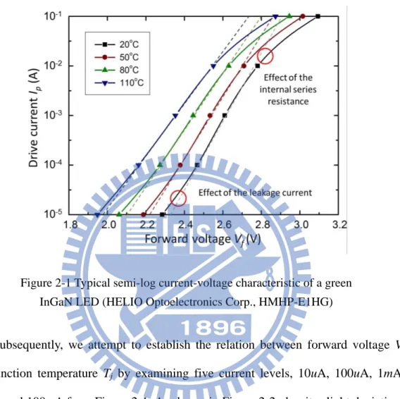
A typical forward current-voltage Ip−Vf characteristic at different junction temperature

Tj is shown in Figure 2-1. According to different current level, the current-voltage

character reveals three different tendencies. When the drive current ≤ 100uA, the current exceeds the exponential fit (dashed line) because the measured character is dominated by various leakage currents. For example, one of these leakages is the carrier tunneling transport across the quantum-well structure . For drive current ≥ 10mA, the effect of the internal series resistance gradually dominate the character of the current-voltage curve, which results in a lower drive current . In the ideal exponential fit region 100uA ≤ Ip ≤ 10mA, the current-voltage characteristic of the p-n

junction diode can be described by the Shockley equation :

exp( f ) P S ideal j eV I I n BT  _(2-2)

The factors e and B indicate the elementary charge and the Boltzmann constant, respectively. I refers to the effective saturation current, the combination of two

saturation currents under diffusion and recombination process. nideal is the ideality

factor with a theoretical value between 1 and 2.

Figure 2-1 Typical semi-log current-voltage characteristic of a green InGaN LED (HELIO Optoelectronics Corp., HMHP-E1HG)

Subsequently, we attempt to establish the relation between forward voltage Vf

and junction temperature Tj by examining five current levels, 10uA, 100uA, 1mA,

10mA, and 100mA from Figure 2-1. As shown in Figure 2-2, despite slight deviations from the linearity due to the effects of leakage current (see the high junction temperature side for current Ip = 100uA) and internal series resistance (see the low

junction temperature side for current Ip = 10mA), a linear approximation has proven to

be sufficient for junction temperature prediction for 100uA ≤ Ip ≤ 10mA , which is

given as:

( ) ( )

f j P j

where γ and δ are the slope for a specific pulsed current IP and the current independent

intercept, respectively.

Figure 2-2 The voltage-temperature characteristic of a green InGaN LED (HELIO Optoelectronics Corp., HMHP-E1HG) at five current levels.

With the linear approximation, the slope γ and intercept δ of Equation (2-3) can be obtained from measuring only two voltage-temperature characteristics, Vf(T1) and

Vf(T2), which prevents a time-consuming measurement. Where T1 and T2 can be the

two extreme cases as the thermal boundary, i.e. T1 = 20 °C and T2 = 110 °C

respectively. Therefore, acalibration curve that profiles the relationship between the forward voltage Vf and junctiontemperatures Tj can be rewritten as:

2 1 1 1 2 1 [ ( )] ( ) ( ) j f f f f T T T V V T T V T V T      (2-4)

For the pulsed drive current Ip > 100mA, the behavior of the internal series

0

( ) ( ) ( )

f j p s j j

V T I R T  I T  _(2-5)

In fact, junction temperature dependence of the internal series Rs(Tj) for Ip > 100mA,

like V(Tj) in the region of 100uA ≤ Ip ≤ 10mA, is often approximated by a linear

expression as well, which could be simply written as Rs(Tj) =γ’Tj +δ’ with slope and

intercept γ’ and δ’. The new slope γ’’ = γ’ + γ and intercept δ’’ = δ’ + δ will be generated to fit the behavior in this region. Consequently, it is more convenient to stick with Equation (2-4) for practical junction temperature estimation, via only two measurements to obtain a set of parameters (γ, δ) or (γ’’, δ’’). The results of the best fitting for all measured LEDs are gathered in Table 2-1. A good agreement between the experimental measurement and linear model can be obtained with R2 exceeding

0.99.

Table 2-1 Pentachromatic LEDs, specific pulsed current Ip , slopes γ and γ’’, and

intercepts δ and δ’’ of the linear approximation.

LED (HELIO

Optoelectronics Corp.)

Ip = 1mA Ip = 100mA

γ δ γ’’ δ’’

HMHP-E1HR (red) -1.91E-03 1.72 -1.82E-03 2.13

HMHP-E1HA (amber) -2.19E-03 1.80 -1.74E-03 2.06

HMHP-E1HG (green) -2.91E-03 2.68 -2.48E-03 3.18

HMHP-E1HB (blue) -1.35E-03 2.43 -1.39E-03 2.82

HMHP-E1HW (cool-white)

2.2 Junction temperature determination

To this point, we have completed junction temperature estimation from the current-temperature calibration measurement. In the following step, sample device is operated under normal conditions, which is exposed to variant ambient temperature Ta

and subjected to a series of DC drive current IDC. With the help of previous calibration,

the junction temperature determination can be achieved in terms of ambient temperature Ta and DC drive current IDC directly.

We firstly apply a constant drive current IDC through the sample LED mounted

on a fixture (Arroyo Instruments, TEC 264-BB-DB9). The entire module is placed inside the cavity of an integrating sphere. The temperature of the fixture controlled by the thermoelectric cooler (Arroyo Instruments, TEC Source 5310) can be regarded as the ambient temperature Ta. As the thermal steady state has been reached, the DC

forward voltage VDC is recorded, and the emitted spectral power distribution SPD as

well as the overall optical power Φ of each sample LED can be captured by the spectrometer (SR-UL1R, Topcon) attached to the integrating sphere. The junction temperature Tj can be determined by the interpolation of the DC forward voltage VDC

according to the pulsed calibration measurement. Finite sampling points are measured in a normal operation range (10 oC ≤ Ta ≤ 100 oC and 0 mA ≤ IDC ≤ 350 mA), in which

the incensements of ambient temperature and DC drive current are programed to be 10 oC and 35 mA, respectively.

Based on the experimental setup, we could have measured results composed of one M x N spectral matrix S and several M x 1 parameter vectors, i.e. tj (junction temperature), ta (ambient temperature),ϕ (optical flux), vDC (DC forward voltage) and

380nm to 780nm in steps of 10nm (N = 41). It is noted that vectors are denoted by bold-faced lower-case letters and matrices are represented by bold-faced capital letters.

With the sufficient database, the junction temperature Tj now can be related to

ambient temperature Ta and DC drive current IDC via the introduction of the equation

developed by A. Keppens : 2 1 2 2 3 4 [ ] ( , ) 1 [ ] t DC DC a j DC a t DC DC R c I c I T T I T R c I c I      (2-6)

where c1, c2, c3, and c4 are fitting parameters that can be easily calculated from

importing variant known input data set (IDC, Ta) and corresponded output data Tj, the

fitting values for all sample devices at Ta = 50 oC are shown in Table 2-2. In Equation

(2-6), the thermal resistance Rt between the junction and the reference point can also

be predetermined by inserting known values of Tj, Ta, Pe (= IDCVDC), and Φ to the

following equation: j a t e T T R P     (2-7)

In which the denominator, the difference of the input electric power Pe and the radiant

flux Φ, indicates the power dissipated in the LED. The measurement results for red AlInGaP LED (HELIO Optoelectronics Corp., HMHP-E1HR) are shown in Table 2-3, where the resistance of 48.1 oC/watt can be determined.

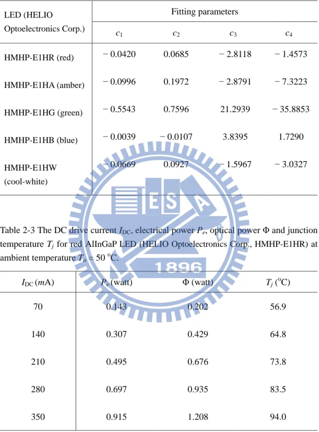
Table 2-2 The values of fitting parameters c1, c2, c3, and c4 for pentachromatic LEDs at ambient temperature Ta = 50 oC. LED (HELIO Optoelectronics Corp.) Fitting parameters c1 c2 c3 c4 HMHP-E1HR (red) − 0.0420 0.0685 − 2.8118 − 1.4573 HMHP-E1HA (amber) − 0.0996 0.1972 − 2.8791 − 7.3223 HMHP-E1HG (green) − 0.5543 0.7596 21.2939 − 35.8853 HMHP-E1HB (blue) − 0.0039 − 0.0107 3.8395 1.7290 HMHP-E1HW (cool-white) − 0.0669 0.0927 − 1.5967 − 3.0327

Table 2-3 The DC drive current IDC, electrical power Pe, optical power Φ and junction

temperature Tj for red AlInGaP LED (HELIO Optoelectronics Corp., HMHP-E1HR) at

ambient temperature Ta = 50 oC.

IDC (mA) Pe (watt) Φ (watt) Tj (oC)

70 0.143 0.202 56.9

140 0.307 0.429 64.8

210 0.495 0.676 73.8

280 0.697 0.935 83.5

2.3 LED spectrum modeling

2.3.1 Double Gaussian model

Generally, the spectral power distribution SPD can be fitted by a single Gaussian function, which incorporates three the power (p), peak wavelength (ˆ) and spectral width (Δλ) with junction temperature. However, in most of cases, practical spectrum is not perfectly symmetric, which will lead to the numerical error by single Gaussian fitting. In order to overcome this issue, in this chapter, we proposed a double Gaussian function with two sets of parameters: ( ,p  ˆ,  ) and ( ',p ˆ', '). On the basis of the discussion in Section 1-2, all parameters related to the spectrum are supposed to be functions of both junction temperature Tj and DC drive current IDC. The estimated

spectrum composed by the double Gaussian function, in contrast with the measured spectrum S, is denoted as S. Therefore, an estimated M x N spectral matrix S (e.g.

M = 100 and N = 41 respectively) for a single-color LED can be expressed as:

'

 

S G G (2-8)

where G g



₁,,g_M



T and G' g



' ,₁ , 'g_M



T represent two Gaussian bases of the double Gaussian spectral matrix. Here we can temporarily omit G' and solely focus on G due to the same treatment for both of them from Equation (2-8) to Equation (2-10). The base matrix G has M spectral vectors g1 to gM, each of them has

N sampling wavelengths. The value for the nth point of mth row vector gm, named as gmn, can be given by:

2 2

ˆ

exp{ [ ( ) ] / }

mn m n m m

where three parameters pm, ˆm, and Δλm refer to the mth Gaussian power, peak

wavelength, and spectral width of the base matrix G, whose values could be found by satisfying the minimization of Equation (2-10) :

2 ˆ ˆ

arg min[ | s_ms_m| , {p_m, _m, _m, p' ,_m ' ,_m ' }]_m (2-10)

where sm is the mth measured spectrum (mth vector) of the spectral matrix S, and '

 

m m m

s g g is the estimated spectrum, corresponding to sm , of the spectral

matrix S .

2.3.2 Single-colour spectral function

After applying the minimization of Equation (2-10) though the spectral matrix, we have three M x 1 vectors including Gaussian power p, peak wavelength ˆλ , and spectral width Δλthat can empirically be related to junction temperature tj and DC drive current iDC: ln(  _{p p} p) M c (2-11a) ˆ λ λ λM c (2-11b) ln(Δλ)M c_{Δλ Δλ} (2-11c) whereMp[tjTln( ) ln(t j iDC) ] l ,Mλ [t j ln(iDC) l] and 1 1/ 2 [ ln( ) ( ) ]  Δλ j j DC M t t i l are

the M x 1 all-ones vector. cp, cλ, and cΔλ refer to 3x1 coefficient vectors, whose values could be calculated by linear least square method, e.g. power coefficient vectorcp  M M



pT p



1MpTln( )p . For the red AlInGaP LED (HMHP-E1HR), Figure 2-3

shows the distribution of all elements in Gaussian power p and its coefficient values

cp1, cp2 and cp3. The corresponded goodness of fit, shown in Figure 2-4, reveals that

the Gaussian power distribution is well fitted by Equation (2-11a).

Similarly, applying the above regularized process Equation (2-9) − Equation (2-11) to the other Gaussian function G' will lead to coefficient vectors

', ', and '

p λ Δλ

c c c . By obtaining all of the coefficients, the complete double Gaussian

function S( ) for single-color LED spectrum can be given in respect of the junction temperature Tj and DC drive current IDC:

2 2 2 2 ( ) ' exp[ ( ) / exp( ) ] exp[ ' ( ') / exp( ') ] S  G G           p p λ λ Δλ Δλ p p λ λ Δλ Δλ m c m c m c m c m c m c (2-12) where m_p[T_jln( ) ln(T_j I_DC) 1] , m_λ [T_j ln(I_DC) 1 ], and m_Δλ[ ln( )T_j T_j 1 (I_DC)1/ 2 1] account for basis vectors of the Gaussian power (P), peak wavelength (ˆ) and spectral width (Δλ) with variables Tj and IDC.

Figure 2-3 The distribution of all elements in Gaussian power p and its fitting

coefficient values cp1, cp2 and cp3.

Figure 2-4 The deviation and goodness of fit for Gaussian power distribution

2.3.3 Phosphor-converted spectral function

For the spectrum of phosphor-converted white LED S_W( ) , the estimated spectrum

( )

W

S  is simply assumed to be composed of two double Gaussian functions S_B( )

and S_F( ) :

( ) ( ) ( )

W B F

S  S  S  (2-13)

where S_B( ) G_BG_B' and S_F( ) G_FG_F' denote the double Gaussian in the blue region and the fluorescence region, respectively. Here a cutoff wavelength λBF should

be defined to denote the boundary in the middle of blue and fluorescence component, whose value can be pointed when the slope of measured spectrum just changes from negative to positive. Therefore, the modeling of the spectrum SB( ) follows the same

mathematical treatment in single-color case from Equation (2-9) to Equation (2-12). The other spectrum S_F( ) , however, can subsequently be found by the same way but using the modified target spectrum|S_W( ) S_B( ) | .

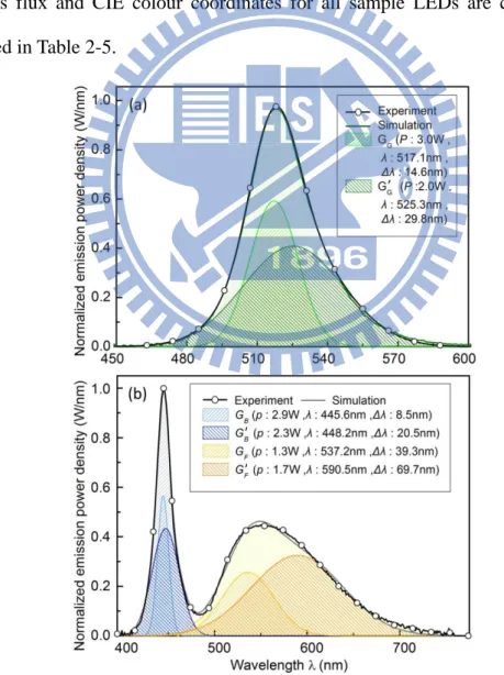
2.4 Validation of the spectral model

In order to validate the spectrum models presented in Equation (2-12) and Equation (2-13). The simulation results as well as the measurement data for green and phosphor-converted LED emission spectra at Tj = 25 oC and IDC = 350 mA are

correspondingly illustrated in Figure 2-5. The results show that a good agreement between the experiment and numerical approximation could be obtained with R2

exceeding 0.98. The fitting parameters of estimated phosphor white light spectrum, determined from Equation (2-11), are to be listed in Table 2-4. Furthermore, the luminous flux and CIE colour coordinates for all sample LEDs are calculated and compared in Table 2-5.

Figure 2-5 The illustration of the simulation model and the experimental measurement

Table 2-4 The parameters of approximated phosphor-converted LED spectrum. The blue and fluorescence components should be individually considered.

( ) ( ) ( ) W B F S  S  S  B G GF GB' GF' 1 p c _{-4.1322 -4.8712} cp1' -4.5411 -4.5641 2 p c _{-0.0051 0.0003} cp2' -0.0010 -0.0009 3 p c _{2.0739 2.2380} cp3' 2.1244 2.1370 1 c_{ 450.0824 539.5471} c1' 453.8196 561.7751 2 c_{ 0.0552 0.0340} c2' 0.0330 -0.0375 3 c_{ -2.0052 0.4289} c3' -2.5025 -4.3316 1 c_ 2.0876 2.9537 c1' 3.6268 4.4596 2 c_ -0.0030 0.0038 c2' 0.0079 0.0022 3 c_ 0.0047 0.0020 c3' 0.0023 0.0053