國
立
交
通
大
學
資訊科學與工程研究所
博
士
論
文
時序資料庫中高效率頻繁樣式探勘演算法之研究
Efficient Algorithms for Mining Frequent Patterns in Temporal
Databases
研 究 生:朱俊榮
指導教授:梁 婷 教授
曾新穆 教授
時序資料庫中高效率頻繁樣式探勘演算法之研究
Efficient Algorithms for Mining Frequent Patterns in Temporal
Databases
研 究 生:朱俊榮 Student:Chun-Jung Chu
指導教授:梁 婷 博士 Advisor:Dr. Tyne Liang
曾新穆 博士
Dr. Vincent Shin-Mu Tseng
國 立 交 通 大 學
資 訊 科 學 與 工 程 研 究 所
博 士 論 文
A Dissertation Submitted to Department of Computer Science
College of Computer Science National Chiao Tung University in partial Fulfillment of the Requirements
for the Degree of Doctor of Philosophy
in
Computer Science January 2008
Hsinchu, Taiwan, Republic of China
時序資料庫中高效率頻繁樣式探勘演算法之研究
學生: 朱俊榮 指導教授: 梁 婷 博士
曾新穆 博士
國立交通大學 資訊科學與工程研究所
摘
要
在資料探勘的領域中,從大型資料庫中尋找資料項目間的頻繁樣式是相當重要之議 題。因為資料項目間的頻繁樣式在現實生活中可應用在許多領域裡,譬如超級市場裡商 品之間的販售關係。然而頻繁樣式所涵蓋的項目廣泛,其中包含了高頻率項目集、新興 高頻率項目集以及高利益項目集等。近年來,由於經濟的關係,市場獲利的需求增加, 新興高頻率項目集與高利益項目集成為主要探討的兩個議題。所謂的新興高頻率項目集 是指項目集在舊有的資料庫中是低頻率項目集,然而在資料庫新增資料後,這些項目集 變成高頻率項目集。至於高利益項目集的探勘,則針對項目集所能得到利益的高低來探 討。過去的研究多著重於如何在大型資料庫中快速且正確地尋找這些項目集,減少候選 項目集的產生、搜尋資料庫的次數以及記憶體的使用等。然而,傳統的演算法無法直接 找尋在時序性資料庫中的頻繁樣式。因此,本論文主旨在研發從時序性資料庫中挖掘出 新興高頻率的項目集以及高利益的項目集的高效率探勘方法。 在新興高頻率項目集的探勘上,我們提出了一個有效率的演算法 EFI (Emerging Frequent Itemsets)-Mine。此演算法利用移動視窗交集法來預測高頻率項目集,因此不需 要像以往的演算法須找出所有的高頻率項目集,以至減少高頻率項目集搜尋所需花費的 時間。實驗的結果,我們所提出的演算法較Apriori 演算法在以 IBM 資料產生器中所產
生的資料情形下,減少90%的執行時間。
此外,在本論文我們也提出一個高利益項目集的演算法THUI (Temporal High Utility
Itemsets)-Mine。此演算法利用分割移動視窗法與交易權重項目集來減少候選項目集的產 生,因此不需要像以往的演算法須找出所有的候選項目集,以至減少搜尋高利益項目集 與資料庫次數所需花費的時間。在以 IBM 資料產生器中所產生的資料下,我們所提出 的演算法較Two-Phase 演算法,執行時間的改善率平均高達 67%。 從利益探勘的特性中,我們可以觀察到資料庫存有許多未滿足門檻值的利益項目 集,有些是值得參考的。我們提出了兩個珍貴的利益項目集之演算法TP-RUI (Two-Phase
Rare Utility Itemsets) -Mine 和 TRUI (Temporal Rare Utility Itemsets) –Mine。尤其是 TRUI-Mine,此演算法利用相對性的門檻值來尋找珍貴的利益項目集,並利用分割移動 視窗法與交易權重項目集來減少候選項目集的產生,以至減少尋找珍貴的利益項目集所 需花費的時間。
由於過去所探討的高利益項目集都是針對正利益的項目來研究,於是我們提出ㄧ個
從大型的資料庫中尋找包含負利益的高利益項目集的演算法 HUINIV (High Utility
Itemsets with Negative Item Values) -Mine。此演算法利用去除負利益項目的交易權重項
目集方法來減少候選項目集產生。實驗的結果,我們所提出的演算法較MEU 演算法在
以IBM 資料產生器中所產生的資料情形下,減少 99%的候選項目集。
Efficient Algorithms for Mining Frequent Patterns in Temporal
Databases
Student: Chun-Jung Chu Advisors: Dr. Tyng Liang
Dr. Vincent Shin-Mu Tseng
Department of Computer Science National Chiao Tung University
ABSTRACT
Mining frequent patterns for discovering the relationship among data items from large databases is an important topic in data mining since frequent patterns can be applied to wide applications. There exist various kinds of frequent patterns like frequent itemsets, emerging frequent itemsets, high utility itemsets and so on. Recently, emerging pattern mining and utility mining become very popular topics because of the rising of economic applications. Emerging frequent itemsets are those who are infrequent in the current database and then become frequent in the new database temporally added with new data transactions. High utility itemsets reveal the utility of an itemset, which can be measured in terms of cost, profit or other expressions of user preferences. In the past, most studies focus on developing efficient and effective methods for finding frequent itemsets from large database by reducing candidate itemsets, database scans and memory space. However, most methods designed for the traditional databases cannot be directly applied for mining temporal patterns in temporal databases because of the high complexity. Hence, we investigate efficient methods for mining emerging frequent itemsets and high utility itemsets in temporal databases in this dissertation.
In emerging pattern mining, a novel approach named EFI (Emerging Frequent
Itemsets)-Mine is presented to effectively identify the potential emerging itemsets by crossing
substantially in mining all frequent itemsets in temporal databases. The experimental results show that EFI delivers 90.6% of improvement over the well-known method Apriori in terms of execution time on various kinds of synthetic datasets.
Besides, we also propose a novel method, namely THUI (Temporal High Utility
Itemsets)-Mine, for mining temporal high utility itemsets from temporal databases efficiently
and effectively. THUI-Mine can effectively identify the temporal high utility itemsets by partitioning sliding window and using transaction-weighted utilization itemsets to generate fewer candidate itemsets such that the execution time and number of database scans can be reduced substantially in mining high utility itemsets from temporal databases. The experimental results show that THUI-Mine delivers 67% of improvement over the well-known method Two-Phase in terms of execution time on various kinds of synthetic datasets.
According to the characters of utility mining, we could obverse some utility itemsets are those itemsets which appear infrequently in the current time window of large databases but are highly associated with specific data. Hence, we proposed two novel algorithms, namely
TP-RUI (Two-Phase Rare Utility Itemsets) -Mine and TRUI (Temporal Rare Utility Itemsets) –Mine, which can effectively identify the temporal rare utility itemsets by using
relative utility threshold. The temporal rare utility itemsets are discovered by partitioning sliding window and using transaction-weighted utilization itemsets to generate fewer candidate itemsets such that the execution time and database scan can be reduced substantially in mining all high and rare utility itemsets in temporal databases.
The past studies on high utility itemsets mining considered only positive item values and ignored the cases of negative item values that may occur in real-life applications. Therefore, we propose a novel method, namely HUINIV (High Utility Itemsets with Negative Item Values)
-Mine, for mining high utility itemsets from large databases with consideration of negative
utility without negative item values to generate fewer candidate itemsets. The experimental results show that HUINIV-Mine delivers 99% of improvement over the well-known method
MEU in terms of candidate itemsets on various kinds of synthetic datasets.
ACKNOWLEGEMENT
(誌 謝)
首先,我最感謝的是我的指導教授梁婷老師以及共同指導教授曾新穆老師,感謝他們在 這四年的研究所生涯中啟發我對學術研究的興趣,並且指導我對論文寫作上的技巧,以 及生活的幫助。在跟隨著梁老師以及曾老師研究的過程中,梁老師以及曾老師對研究的 執著以及熱忱,一直是我學習的榜樣。此外,還要感謝李素瑛教授和彭文志教授在計畫 書口試、校內口試以及校外口試時提供許多寶貴的意見。 感謝口試委員:東華資管系楊維邦教授、中央資工系洪炯宗教授、逢甲資工系楊東 麟教授、清大資工系陳宜欣教授在口試過程中提供許多寶貴的建議,讓我的論文能更趨 完善。諸位口試委員都是我在學術研究的道路上的最佳學習典範。資訊擷取實驗室的同 學和學弟妹是我博士班研究生涯的好伙伴,謝謝大家也祝福學弟妹們早日收穫豐富的研 究成果,再次謝謝你們在這段過程中對我的幫忙以及鼓勵。 最後要感謝的是一直支持我的家人,有你們的支持與鼓勵,讓我在求學的過程中能 無憂無慮且專心的在學術研究上,謝謝你們。 要感謝的人太多,僅在此對所有曾經幫助過我的朋友們,致上我真切的謝意。 僅以此論文,獻給我最親愛的家人。TABLE OF CONTENTS
ABSTRACT ...iii
ACKNOWLEGEMENT ...vi
TABLE OF CONTENTS ...vii
LIST OF FIGURES ...viii
LIST OF TABLES ...ix
Chapter 1 Introduction ... 1
1.1 Motivation and Research Goal ...2
1.2 Related Work ...3
1.3 Organization of Thesis...6
Chapter 2 Mining Temporal Emerging Itemsets from Temporal Databases ... 8
2.1 Problem Definition ...8
2.2 Mining Temporal Emerging Itemsets...13
2.3 Experiments and Analysis ...20
Chapter 3 Mining Temporal High Utility Itemsets from Temporal Databases...26
3.1 Problem Definition ...26
3.2 Proposed Method...30
3.3 Experiments and Analysis ...42
Chapter 4 Mining Temporal Rare Utility Itemsets in Large Databases Using Relative Utility Thresholds ... 51
4.1 Problem Definition ...51
4.2 Proposed Methods ...55
4.3 Experiments and Analysis ...69
Chapter 5 Mining High Utility Itemsets with Negative Item Values... 77
5.1 Problem Definition ...77
5.2 Proposed Method...81
5.3 Experiments and Analysis ...88
Chapter 6 Conclusions and Future Work... 98
LIST OF FIGURES
Figure 2-1. An example of online transaction flows. ...9
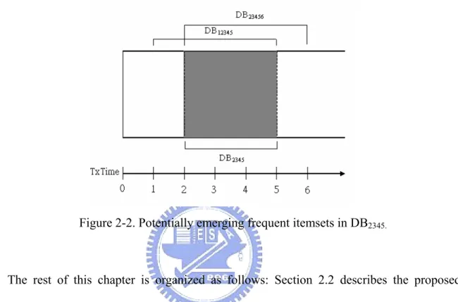
Figure 2-2. Potentially emerging frequent itemsets in DB2345...13
Figure 2-3. Emerging frequent itemsets. ...15
Figure 2-4. Potentially emerging frequent itemsets...16
Figure 2-5. Potentially emerging frequent itemsets for temporal patterns. ...18
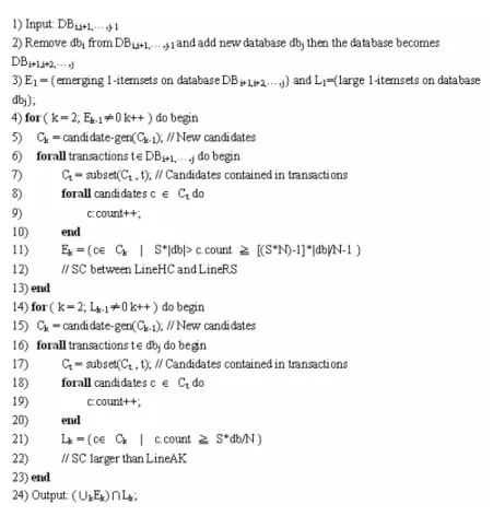
Figure 2-6. Algorithm of EFI-Mine...19
Figure 2-7. Accuracy under different support values (N100T5C1000, W=10)...22
Figure 2-8. Execution time with w=10...23
Figure 2-9. Accuracy under different window sizes...24
Figure 2-10. Accuracy under different numbers of items per transaction with w=10...24
Figure 2-11. Accuracy under different numbers of items...25
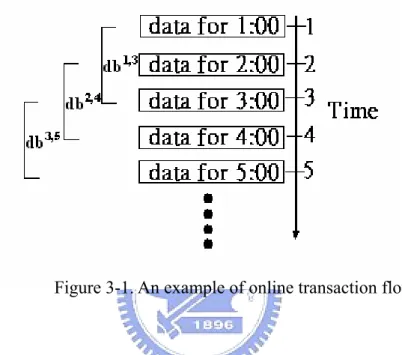
Figure 3-1. An example of online transaction flows. ...27
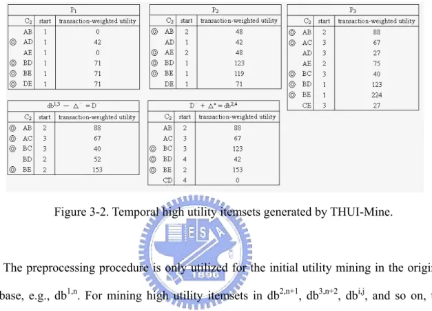
Figure 3-2. Temporal high utility itemsets generated by THUI-Mine...35
Figure 3-3. Preprocessing procedure of THUI-Mine. ...40
Figure 3-4. Incremental procedure of THUI-Mine...42
Figure 3-5. Utility value distribution in utility table. ...44
Figure 3-6. Execution time for Two-Phase and THUI on T20.I6.D100K.d10K. ...47
Figure 3-7. Execution time for Two-Phase and THUI on T10.I6.D100K.d10K. ...48
Figure 3-8. Scale-up performance results for THUI vs. Two-Phase. ...49
Figure 3-9. Execution time for Two-Phase and THUI on gazelle dataset. ...50
Figure 4-1. Temporal rare utility itemsets generated by TRUI-Mine...61
Figure 4-2. Preprocessing procedure of TRUI-Mine...67
Figure 4-3. Incremental procedure of TRUI-Mine...69
Figure 4-4. Utility value distribution in utility table. ...71
Figure 4-5. Execution time on T10.I6.D100K.d10K...74
Figure 4-6. Execution time on T20.I6.D100K.d10K...74
Figure 4-7. Execution time on T10.I4.D100K.d10K...75
Figure 4-8. Scale-up performance results...75
Figure 5-1. High utility itemsets generated from large databases by HUINIV-Mine...86
Figure 5-2. Procedure used by HUINIV-Mine. ...88
Figure 5-3. Utility value with negative distribution in utility table...90
Figure 5-4. Execution time for HUINIV on T20.I6.D100K and T10.I6.D100K...94
Figure 5-5. Execution time for HUINIV on T20.I4.D100K and T10.I4.D100K...95
LIST OF TABLES
Table 2-1. The support values of the inter-transaction itemset {c, g}. ... 11
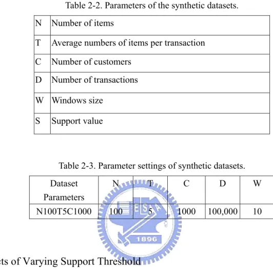
Table 2-2. Parameters of the synthetic datasets...21
Table 2-3. Parameter settings of synthetic datasets. ...21
Table 3-1. A transaction database and its utility table. ...28
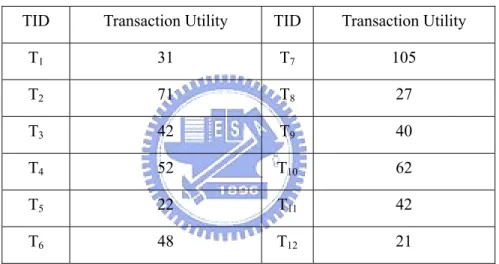
Table 3-2. Transaction utility of the transaction database. ...34
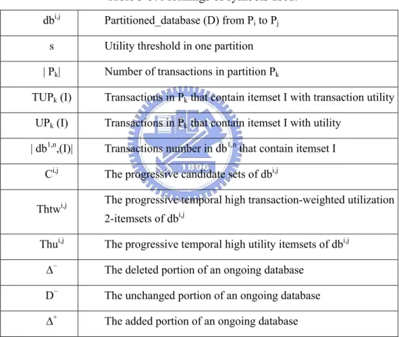
Table 3-3. Meanings of symbols used. ...38
Table 3-4. The number of candidate itemsets generated on database T10.I6.D100K.d10K. ...45
Table 3-5. The number of candidate itemsets generated on database T20.I6.D100K.d10K. ...46
Table 4-1. A transaction database and its utility table. ...53
Table 4-2. Transaction utility of the database...57
Table 4-4. Number of candidate itemsets, temporal high utility itemsets and temporal rare utility itemsets generated on dataset T10.I6.D100K.d10K. ...72
Table 5-1. A transaction database and its utility table. ...78
Table 5-2. Transaction utility of the transaction database. ...84
Table 5-3. Transaction utility without negative item values of the transaction database. ...85
Table 5-4. Meanings of symbols used. ...87
Table 5-5. The number of candidate itemsets and high utility itemsets generated from database T10.I4.D100K...92
Table 5-6. The number of candidate itemsets and high utility itemsets generated from database T10.I6.D100K...92
Table 5-7. The number of candidate itemsets and high utility itemsets generated from database T20.I4.D100K...93
Table 5-8. The number of candidate itemsets and high utility itemsets generated from database T20.I6.D100K...93
Table 5-9. Database BMS-POS characteristics. ...96
Table 5-10. The number of candidate itemsets and high utility itemsets generated on database BMS-POS. ...97
Chapter 1
Introduction
The mining of association rules for finding the relationship between data items in large databases is a well studied technique in data mining field with representative methods like
Apriori [1][2][7]. An important research issue extended from the association rules mining is
the discovery of temporal association patterns in temporal databases due to the wide applications on various domains. Temporal data mining can be defined as the activity of looking for interesting correlations or patterns in large sets of temporal data accumulated for other purposes [6]. For a database with a specified transaction window size, we may use the algorithm like Apriori to obtain frequent itemsets from the database.
For time-variant temporal databases, there is a strong demand to develop an efficient and effective method to mine various temporal patterns [13]. However, most methods designed for the traditional databases cannot be directly applied for mining temporal patterns in temporal databases because of the high complexity.
In many applications, the frequency of an itemset may not be a sufficient indicator of interestingness, because it only reflects the number of transactions in the database that contain the itemset. It does not reveal the utility of an itemset, which can be measured in terms of cost, profit or other expressions of user preferences. On the other hand, frequent itemsets may only contribute a small portion of the overall profit, whereas non-frequent itemsets may contribute a large portion of the profit. In reality, a retail business may be interested in identifying its most valuable customers (customers who contribute a major fraction of the profits to the company). Hence, frequency is not sufficient to answer questions such as whether an itemset is highly profitable, or whether an itemset has a strong impact. Utility mining is thus useful in a wide range of practical applications and was recently studied in [8][21][35].
1.1 Motivation and Research Goal
The research objective of this dissertation is to investigate algorithms for mining emerging frequent itemsets and high utility itemsets efficiently and effectively.
The first research issue of this dissertation is mining temporal emerging frequent itemsets from temporal databases efficiently and effectively, we propose a new method, namely EFI (Emerging Frequent Itemsets)-Mine. The temporal emerging frequent itemsets are those that are infrequent in current time window of database but have high potential to become frequent in the subsequent time windows. Discovery of emerging frequent itemsets is an important process for mining interesting patterns like association rules from temporal databases. The novel contribution of EFI-Mine is that it can effectively identify the potential emerging itemsets such that the execution time can be reduced substantially in mining all frequent itemsets in temporal databases. This meets the critical requirements of time and space efficiency for mining temporal databases.
Furthermore, we propose a novel method, namely THUI (Temporal High Utility
Itemsets)-Mine, for mining temporal high utility itemsets from temporal databases efficiently
and effectively. The novel contribution of THUI-Mine is that it can effectively identify the temporal high utility itemsets by generating fewer candidate itemsets such that the execution time can be reduced substantially in mining all high utility itemsets in temporal databases. In this way, the process of discovering all temporal high utility itemsets under all time windows of temporal databases can be achieved effectively with less memory space and execution time. This meets the critical requirements on time and space efficiency for mining temporal databases.
According to the characters of utility mining, we could obverse some utility itemsets are those itemsets which appear infrequently in the current time window of large databases but are highly associated with specific data. Hence, we proposed two novel algorithms, namely
TP-RUI (Two-Phase Rare Utility Itemsets) -Mine and TRUI (Temporal Rare Utility Itemsets) –Mine, which can effectively identify the temporal rare utility itemsets by using
relative utility threshold. The novel contribution of TRUI-Mine is particularly that it can effectively identify the temporal rare utility itemsets by generating fewer temporal high transaction-weighted utilization 2-itemsets in temporal databases. In this way, the process under all time windows of temporal databases can be achieved effectively with limited memory space, less candidate itemsets and CPU I/O time.
The final issue explored in this thesis is based on the observation that the past studies on high utility itemsets mining considered only positive item values and ignored the cases of negative item values that may occur in real-life applications. Therefore, we propose a novel method, namely HUINIV (High Utility Itemsets with Negative Item Values) -Mine, for mining high utility itemsets from large databases with consideration of negative item values. The novel contribution of HUINIV-Mine is that it can effectively identify high utility itemsets by generating fewer high transaction-weighted utilization itemsets such that the execution time can be reduced substantially in mining the high utility itemsets. In this way, the process of discovering all high utility itemsets with consideration of negative item values can be accomplished effectively with less requirements on memory space and CPU I/O. This meets the critical requirements of temporal and spatial efficiency for mining high utility itemsets with negative item values.
1.2 Related Work
In association rules mining, Apriori [1], DHP [24], and partition-based ones [20][27] are proposed to find frequent itemsets. Many important applications have called for the need of incremental mining. This is due to the increasing use of the record-based databases whose data are being continuously added. Many algorithms like FUP [24], FUP2 [11] and UWEP
[4][5] are proposed to solve incremental database for finding frequent itemsets. The FUP algorithm updates the association rules in a database when new transactions are added to the database. Algorithm FUP is based on the framework of Apriori and is designed to discover the new frequent itemsets iteratively. The idea is to store the counts of all the frequent itemsets found in a previous mining operation. Using these stored counts and examining the newly added transactions, the overall count of these candidate itemsets are then obtained by scanning the original database. An extension to the work in [10] was reported in [11] where the authors propose an algorithm FUP2 for updating the existing association rules when
transactions are added to and deleted from the database. UWEP (Update With Early Pruning) is an efficient incremental algorithm, that counts the original database at most once, and the increment exactly once. In addition the number of candidates generated and counted is minimum.
In recent years, processing data from data streams is a very popular topic in data mining. A number of algorithms like Lossy Counting [22], FTP-DS [30] and RAM-DS [31] have been proposed to process data in data streams. Lossy Counting divided incoming stream conceptually into buckets. It uses bucket boundaries and maximal possible error to update or delete the itemsets with frequency for mining frequent itemsets. FTP-DS is a regression-based algorithm to mine frequent temporal patterns for data streams. A wavelet-based algorithm, called algorithm RAM-DS, to perform pattern mining tasks for data streams by exploring both temporal and support count granularities.
Some algorithms like SWF [18] and Moment [12] are proposed to find frequent itemsets over a stream sliding window. By partitioning a transaction database into several partitions, algorithm SWF employs a filtering threshold in each partition to deal with the candidate itemset generation. Moment algorithm use the closed enumeration tree (CET), to maintain a dynamically selected set of itemsets over a sliding window.
significantly between two databases. We view emerging frequent itemsets as a special case of the emerging patterns described by Dong and Li. Recently, a new algorithm modifies an existing incremental algorithm, UWEP, so that it can identify emergent large itemsets. It uses incremental scheme for finding emerging frequent itemsets [28].
A formal definition of utility mining and theoretical model was proposed in [35], namely MEU, where the utility is defined as the combination of utility information in each transaction and additional resources. Since this model cannot rely on downward closure property of Apriori to restrict the number of itemsets to be examined, a heuristic is used to predict whether an itemset should be added to the candidate set. However, the prediction usually overestimates, especially at the beginning stages, where the number of candidates approaches the number of all the combinations of items. The examination of all the combinations is impractical, either in computation cost or in memory space cost, whenever the number of items is large or the utility threshold is low. Although this algorithm is not efficient or scalable, it is by far the best one to solve this specific problem.
Another algorithm named Two-Phase was proposed in [21], which is based on the definition in [35] and achieves the finding of high utility itemsets. The Two-Phase algorithm is used to prune down the number of candidates and can obtain the complete set of high utility itemsets. In the first phase, a model that applies the “transaction-weighted downward closure property” on the search space is used to expedite the identification of candidates. In the second phase, one extra database scan is performed to identify the high utility itemsets. However, this algorithm must rescan the whole database when new transactions are added from temporal databases. It incurs more cost on I/O and CPU time for finding high utility itemsets. Hence, the Two-Phase algorithm is focused on traditional databases and is not suited for mining temporal databases.
Many algorithms were proposed for mining useful information on different applications. A mining method was proposed to process computer vulnerability [38] for finding
vulnerability correlation. A heuristic reduction algorithm HeuriRed and A complete heuristic reduction algorithm HeuriComRed [29] based on discernibility matrix were proposed to process imprecise and incomplete data for attributes reduction mining.
One algorithm named RSAA (Relative support Apriori Algorithm) [36] is a method to discover the association rules for significantly rare itemsets that appear infrequently in the database but are highly associated with specific data. The technique adopts a new criterion, relative support, which can identify the strong co-relation of the significant rare itemset items with the specific data co-occurring in relatively high proportion. However, the technique of this algorithm can not be adopted in utility mining because it violates definitions of utility mining. Hence, the RSAA algorithm is focused on traditional association rules discovery and databases, and so it is not suited for utility mining and temporal databases.
Although there existed numerous studies on frequent itemsets mining and data stream analysis as described above, there is no algorithm proposed for finding emerging frequent itemsets, temporal high utility itemsets, temporal rare utility itemsets and high utility itemsets with negative item values in temporal and large databases. This motivates our exploration on the issue of efficiently mining various frequent itemsets we describe above in temporal databases like data streams in this research. Therefore, we propose four methods that can identify frequent pattern efficiently and effectively. To our best knowledge, this is the first work on mining t emerging frequent itemsets, temporal high utility itemsets, temporal rare utility itemsets and high utility itemsets with negative item values from temporal and large databases.
1.3 Organization of Thesis
The remainder of this thesis is organized as follows. In Chapter 2, we describe EFI-Mine algorithm for mining temporal emerging frequent itemsets from temporal databases efficiently
and effectively. Efficient THUI-Mine algorithm for mining temporal high utility itemsets from temporal databases is introduced in Chapter 3. In Chapter 4, we describe two novel algorithms, namely TP-RUI (Two-Phase Rare Utility Itemsets) -Mine and TRUI (Temporal Rare Utility
Itemsets) –Mine, for mining temporal rare utility itemsets from temporal databases. relevance
feedback methods are surveyed and a novel feedback mechanism is proposed. In Chapter 5, we address a novel method, namely HUINIV (High Utility Itemsets with Negative Item
Values) –Mine, for efficiently and effectively mining high utility itemsets from large databases
Chapter 2
Mining Temporal Emerging Itemsets from
Temporal Databases
2.1 Problem Definition
The mining of association rules for finding the relationship between data items in large databases is a well studied technique in data mining field with representative methods like
Apriori [1][2][7]. The problem of mining association rules can be decomposed into two steps.
The first step involves finding all frequent itemsets (or say large itemsets) in databases. Once the frequent itemsets are found, generating association rules is straightforward and can be accomplished in linear time.
An important research issue extended from the association rules mining is the discovery of temporal association patterns in temporal databases due to the wide applications on various domains. Temporal data mining can be defined as the activity of looking for interesting correlations or patterns in large sets of temporal data accumulated for other purposes [6]. For a database with a specified transaction window size, we may use the algorithm like Apriori to obtain frequent itemsets from the database. For time-variant temporal databases, there is a strong demand to develop an efficient and effective method to mine various temporal patterns [4]. However, most methods designed for the traditional databases cannot be directly applied for mining temporal patterns in temporal databases because of the high complexity.
Without loss of generality, consider a typical market-basket application as illustrated in [30] has been considered. The transaction flow in such an application is shown in Figure 2-1 where items a to g stand for items purchased by customers.
Figure 2-1. An example of online transaction flows.
In Figure 2-1, for example, the third customer bought item c during time t=[0,1), items c, e and g during t=[2, 3), and item g during t=[4, 5). It can be seen that in such a data stream environment it is intrinsically difficult to conduct the frequent pattern identification due to the limited time and space constraints. Furthermore, it wastes too much times finding frequent itemsets in different window times. Therefore, we develop a new scheme to find potential emerging frequent itemsets before next window times.
Dong and Li [14] define an emerging pattern as an itemset the support of which increases significantly between two databases. We view emerging frequent itemsets as a special case of the emerging patterns described by Dong and Li. An Emerging Frequent
Itemset (EFI) can be considered as an itemset that is infrequent (i.e., small) in the current
database and gets increased for its support so that it will eventually become frequent (i.e., large) in the new database temporally added with new data transactions. For example, in the market basket domain, we may assume an interval as the time between wholesale purchases. Recognizing the set of items that will emerge or become frequent in the next time period with windows size may allow the storekeeper to order these emerging items much earlier than usual. Thus, the storekeeper will know what kinds of items will be popular in the next time period and avoid losing the income that their sales could have generated. Although some
related issues like mining emerging frequent itemsets [28] and incremental frequent itemsets [9][10][11][25] have been studied, they have been focused on traditional databases and are not suited for temporal databases.
In this chapter, we explore the issue of efficiently mining emerging frequent itemsets in temporal databases like data streams [15][16][17][19]. We propose an algorithm named
EFI-Mine that can discover emerging frequent itemsets from temporal databases efficiently
and effectively. The EFI-Mine algorithm is based on the concept of Apriori algorithm [2] for mining frequent itemsets. The novel contribution of EFI-Mine is that it can effectively identify the potential emerging frequent itemsets in temporal databases so that the execution time for mining frequent itemsets can be substantially reduced. That is, EFI-Mine can discover the itemsets that are infrequent in current time window but will become frequent ones with high probability in subsegment time windows. In this way, the process of discovering all frequent itemsets under all time windows of temporal databases can be achieved efficiently with limited memory space. This meets the critical requirements of time and space efficiency for mining temporal databases. Through experimental evaluation,
EFI-Mine is shown to deliver high precision in finding the emerging frequent itemsets and it
also achieves high scalability in terms of execution time.
Support Framework for Mining Temporal Patterns
In this chapter, the mining of temporal patterns are explored for illustrative purposes since not only the patterns should be efficiently and effectively extracted but also variations of corresponding occurrence frequencies should be tracked. In market-basket analysis, patterns along with their frequencies are extracted from sliding window in transactions. So the data expires after a user-specified time window. As time advances, new data is included while obsolete data is discarded. With the mining task for discovering frequent temporal patterns,
only patterns with occurrence frequencies no less than a specified threshold are being tracked. We focus in this chapter on handling the different sliding windows to find emerging frequent itemsets.
An example showing the basic process in transforming transactions into numerical time series, for discovering frequent temporal patterns, is provided as follows.
Example 1: Consider the transaction flows shown in Figure 2-1. Given the window size w=3
and the minimum support value as 40%, occurrence frequencies of the inter-transaction itemset {c, g} from time t=1 to t=5 can be obtained as shown in Table 2-1.
Table 2-1. The support values of the inter-transaction itemset {c, g}. TxTime Occurrence(s) of {c,g} Support
t=1 t=2 t=3 t=4 t=5 w[0,1] w[0,2] w[0,3] w[1,4] w[2,5] none CustomerID={2, 4} CustomerID={2, 3, 4} CustomerID={2, 3} CustomerID={1, 3, 5} 0 2/5=0.4 3/5=0.6 2/5=0.4 3/5=0.6
With the sliding window model, the frequent temporal patterns can be discovered for different time windows. The main goal of our research is to discover interesting emerging itemsets under progressive time windows.
Emerging Frequent Itemsets and Interesting Emerging Itemsets
In a database, the frequent itemsets will be changed when new datum are added. As time progress, we can see many interesting patterns with regards to the change in status of individual itemsets. An itemset that was infrequent may become frequent (large), while frequent itemsets may become infrequent (small) and an itemset may remain frequent or infrequent. We define infrequent itemsets that are moving toward being frequent as emerging. Conversely, frequent itemsets moving toward infrequent are submerging. An infrequent
(frequent) itemset that becomes large, i.e. with support above (below) minimum support value, is said to have emerged (submerged). The problems we address in this chapter are: 1) How can we identify itemsets that are emerging (submerging)? 2) Which of these itemsets have the potential to emerge (submerge) within the next time window? That is, we focus on finding emerging frequent itemsets in this chapter.
According to the emerging itemsets of incremental scheme, we develop this concept on the temporal data mining. Temporal data mining has the limitation on window size for finding emerging itemsets. Therefore, we must change the formula for finding emerging itemsets. For the remainder of this chapter, we give definitions to the formula.
Definition 2.1 dbk is the transactions in t=k, i.e., db1 is the transactions in t=1.
Definition 2.2 DBi,i+1,…,j is the transactions in t=i to j, i.e., DB12345 is the transactions in t=1 to 5. We also view DB12345 as the accumulation of db1+db2+db3+db4+db5.
Suppose the original database is DBi,i+1,…,j with window size=N and N=j-i+1. Due to the
limitation of window size, we should discard the old database dbi when adding a database
dbj+1. The new database should be DBi+1,i+2,…,j+1. In our scheme, we should find emerging
itemsets before a new database is added. So we should focus on the database DBi+1,i+2,…,j.
The old database dbi is useless for finding emerging itemsets. For example, suppose original
database is DB1234 and we set the limitation of window size as 5. If a database db5 is added,
the new database will be DB12345. Due to the limitation of window size, when adding a
database db6, we should discard the old database db1. Thus, the new database becomes
DB23456. In our scheme, we would find potential emerging frequent itemsets before a database
is added. So we should focus on the database DB2345 finding potential emerging frequent
itemsets. And the potential emerging frequent itemsets of the database DB2345 can be
represented more accurate in the new database DB23456. In practice, with the feature of data
stream, we first remove db1 from DB1234 and then add db5 to form the database DB2345. So we
database db6 to form DBB23456, and this conforms the limitation of window size. Figure 2-2 shows we would find potential emerging frequent itemsets from the database DB2345. So the
window size should be N-1 for finding potential emerging itemsets.
Figure 2-2. Potentially emerging frequent itemsets in DB2345.
The rest of this chapter is organized as follows: Section 2.2 describes the proposed approach, EFI-Mine, for finding the emerging frequent itemsets. In section 2.3, we describe the experimental results for evaluating the proposed method. The conclusion of the chapter is provided in Section 2.4.
2.2 Mining Temporal Emerging Itemsets
In this Section, we give an example for mining temporal emerging itemsets from data stream. The proposed algorithm, EFI-Mine, is also described in details in this Section.
An example for mining emerging itemsets
Figure 2-3 shows an example of emerging itemsets modified on that proposed by Dong and Li in [14] for the special case of EFI. It shows partitions of the space of itemsets, indicating all
possible transitions for an itemset X from original database DB to the new database DB+db. Figure 2-3 plots the support count in DB (denoted as SCDB) against the support count in
db (denoted as SCdb). Each point in the graph depicts an ordered pair (SCdb, SCDB) where the
sum of SCdb and SCDB is an itemset's support count in DB+db at some increment interval. If
the increment adds no transactions to an itemset's support count, then its support count in DB has to be equal to minSCDB+minSCdb in order to achieve minSCDB+db. This corresponds to
point H in Figure 2-3. Alternatively, if an itemset's SC is equal to |db| in db, then its support in DB has to be some SC=n, where n>0, and n= minSCDB+minSCdb -|db| for the itemset to be
frequent. This is point C in Figure 2-3. Line HC partitions the space of all itemsets in DB+db into frequent and infrequent. The shaded area in Figure 2-3 represents all the frequent itemsets and it includes Line HC. Specific partitions under HC contain itemsets that are emerging in the current increment. For example, the area defined by ΔHFG represents those itemsets that were frequent itemsets in DB, infrequent itemsets in db, and now are infrequent in DB+db. These itemsets have therefore submerged. ΔGIC represents itemsets that were infrequent in DB and frequent in db. These itemsets have emerged. Therefore, we can find all itemsets in area ABCG are emerging in the current interval and all itemsets in area OAGH are submerging.
Figure 2-3. Emerging frequent itemsets.
However, there are too many emerging itemsets in area ABCG. In fact, we should focus more potential emerging itemsets. To have the potential to emerge in the next increment, the support count of the itemset in DB+db needs to be greater than or equal to 2minSCdb+minSCDB - |db| in the current increment. All points with this value are represented
by line RS in Figure 2-4.
For example, if we have a database with |DB|= 10000, |db|= 1000 and minsup =0.2, then the minimum support count for the current increment is 2,200 (2,000 from DB plus 200 from db). If an itemset can add the maximum support incremental support count, a total of 1,000 from db, in the next increment, it would need a support count of at least 1400 in the current increment to be able to attain the minimum support count of 2,400 ((11000+1000)*0.2=2400) needed to become frequent.
The band of itemsets between line RS and line HC are all itemsets that have the potential to become frequent in the next increment, by this formula. Intersecting area ABCG and HCSR, we get itemsets in GDSC are most likely to emerge in the next increment.
Figure 2-4. Potentially emerging frequent itemsets.
Algorithm of EFI-Mine
With window size we mention in Section 2.2.2 and the concepts of emerging itemsets in section 2.3.1, we set support value as S and assume the original database as DBi,i+1,…,j-1.
According to the scheme we mentioned previously, if we want to find frequent itemsets from
DBi+1,i+2,…,j+1, we should focus on DBi+1,i+2,…,j for finding potential emerging frequent
itemsets after adding database dbj and then find potential emerging frequent itemsets of the
database DBi+1,i+2,…,j+1 before adding next incremental new database dbj+1. It means dbi
would be an old database that needs not be considered. After adding new database dbj+1, the
new database would be DBi+1,i+2,…,j+1. So the window size is N when database is changed
from dbi+1 to dbj+1. It also indicates N=(j+1)-(i+1)+1. By the feature of temporal data mining,
we set |db|=|dbi|=|dbi+1|=…=|dbj|. In Figure 2-4, various lines bear the following meaning:
j j i i db DB SC SC
LineHC=min +1,+2,...,−1 +min
1 ,..., 2 , 1 min + + − = j i i DB SC LineFI
| | min min 2 1 ,..., 2 , 1 j DB db SC db SC LineRS j i i j+ − = + + − | | min min 1 ,..., 2 , 1 j DB db SC db SC LineEC j i i j+ − = + + − dbj SC LineAK min=
According to the feature of window size in temporal mining, incremental database means adding length of original transactions and also promoting the probability of infrequent itemsets to become frequent. Because we focus on N-1 window size for finding potential emerging frequent itemsets, these formulas should be divided by N-1 base on the number of database as follows: 1 / ) min (min 1, 2,..., 1 + − = SC + + − SC N LineHC j j i i db DB 1 -)/N | | min min 2 ( 1 ,..., 2 , 1 j DB db SC db SC LineRS j i i j + − = + + −
Because line FI does not add new database, it should be divided by (N-1)-1. It means line FI should be divided by N-2 as follows:
2 -/N min 1 ,..., 2 , 1+ − + = j i i DB SC LineFI
Line EC means that adding new database dbj and an itemset's SC is equal to |dbj| in dbj,
so it should be divided by (N-1) as follows: 1 -)/N | | min min ( SCdb SCDB1, 2,..., 1 dbj LineEC j i i j + − = + + −
Because dbj belongs to one of N window size, the formula should be divided by N as
follows:
N SC LineAK=min dbj/
Figure 2-5 illustrates the potentially emerging frequent itemsets in area GDSC with window size limitation. The formula for each line is as mentioned above.
According to these formulas, we can simplify these lines as follows: HC=[S*(j-1-(i+1)+1)*|db|+S*|db|]/N-1= [S*(N-2)*|db|+S*|db|]/N-1= S*|db|
FI= [S*(j-1-(i+1)+1)|db|]/N-2= S*|db| RS=[2*S*|db|+S*[(j-1)-(i+1)+1]*|db|-|db|]/N-1= [2*S*|db|+S*(N-2)*|db|-|db|]/N-1= [(S*N)-1]*|db|/N-1 EC=[S*|db|+S*[(j-1)-(i+1)+1]*|db|-|db|]/N-1= [S*|db|+S*(N-2)*|db|-|db|]/N-1= [S*(N-1)-1]*|db|/N-1 AK=S*db/N
We can also find potentially emerging frequent itemsets in area HRSC without concerning support count in dbj. However, it will reduce the accuracy with potentially
emerging frequent itemsets. Taking into consideration of dbj would get the trend of itemsets
and get better accuracy with potentially emerging frequent itemsets. Therefore, itemsets in GDSC are most likely to emerge in the next increment.
Figure 2-5. Potentially emerging frequent itemsets for temporal patterns.
Figure 2-6 shows the algorithm of EFI-Mine and the processing procedure is outlined below. The basic processing procedure is like Apriori except the definition of for minimum support value for finding temporal emerging itemsets from data stream. With window size N, we would not only remove dbi but also add new database dbj for finding 1-emerging itemsets
on the database DBi+1,i+2,…,j and finding large 1-itemsets on the database dbj from Step 1 to
Step 3. So the purpose is to find potential emerging frequent itemsets of the database
DBi+1,i+2,…,j+1 before adding next new database dbj+1. We generate k-candidates and find
k-emerging itemsets by calculating support count as mentioned previously from Step 4 to Step 13. Then, we generate k-candidates and find k-large itemsets by support count we mention from Step 14 to Step 23. Finally, those itemsets meeting the constraints S*|db|> c.count ≧ [(S*N)-1]*|db|/N-1 on DBBi+1,i+2,…,j and c.count S*db/N db≧ j are obtained as the potentially emerging frequent itemsets.
Figure 2-6. Algorithm of EFI-Mine.
We may utilize the formulas mentioned before to discuss the following situations. Notice that an itemset is emerging or not depends on support count of the itemset. Given an itemset whose support counts in DBi+1,i+2,…,j-1 and DBi+1,i+2,…,j-1+dbj are and
1 ,..., 2 , 1 DB SC + + − j i i
j j i i+1,+2,...,−1+db
DB
SC , respectively, the growth rate of that itemset is .
The growth rate of an itemset that maintains minimal support
is . An itemset meeting the
1 ,..., 2 , 1 1 ,..., 2 , 1 DB DB -SC SC i+i+ j−+dbj i+i+ j− 1 ,..., 2 , 1 1 ,..., 2 , 1 DB DB -minSC minSC i+ i+ j−+dbj i+ i+ j− 1 minSC -minSC SC -SC 1 ,..., 2 , 1 1 ,..., 2 , 1 1 ,..., 2 , 1 1 ,..., 2 , 1 DB DB DB DB > − + + − + + − + + − + + + + j i i j j i i j i i j j i i db db
is an emerging itemset. An itemset needs a support
count of at least db db db j i i j j j i i DB 2 DB 1, 2,..., 1 1 minSC 1, 2,..., 1 minSC + + + − + + + − +
+ = to emerge in adding a new
database dbj+1 with expanding one window size. A potential emerging frequent itemset is the
one that is emerging and meets the following constraint: . Hence, we can infer that an itemset that will
potentially emerge with expanding n window sizes is an itemset that is currently emerging
and . Of course, the larger n is, the less
accurate with finding potential emerging frequent itemsets might be.
db db dbj i i j j i i j i i j j i i DB DB DB 2 DB1, 2,..., 1 (SC 1, 2,..., 1 -SC 1, 2,..., 1) minSC 1, 2,..., 1 SC ++ −+ + + + −+ + + − > ++ − + ndb db dbj i i j j i i j i i j j i i+1,+2,...,−1+ +n DB+1,+2,...,−1+ DB+1,+2,...,−1 > DB+1,+2,...,−1+ DB (SC -SC ) minSC SC
2.3 Experiments and Analysis
To evaluate the performance of EFI-Mine, we conducted experiments of using synthetic dataset generated via a randomized transaction generation algorithm in [3]. The synthetic data generation program takes the parameters as shown in Table 2-2, and the values of parameters used to generate the datasets are shown in Table 2-3. The simulation is implemented in C++ and conducted in a machine with 1.4GHz CPU and 512MB memory. The main performance metrices used are execution time and accuracy. We recorded the execution time that EFI-Mine spends in finding potential emerging frequent itemsets. The accuracy is to measure the number of actual emerging frequent itemset in ratio of the total potential emerging frequent itemsets that we found. Hence, the accuracy is defined as follows:
frequent itemsets)
Table 2-2. Parameters of the synthetic datasets. N Number of items
T Average numbers of items per transaction C Number of customers
D Number of transactions W Windows size
S Support value
Table 2-3. Parameter settings of synthetic datasets. Dataset
Parameters
N T C D W
N100T5C1000 100 5 1000 100,000 10
Effects of Varying Support Threshold
The proposed approach is verified with experiments in various measurements. We vary the values of support threshold from 30% to 70% for interesting the effects on the accuracy. The other parameters were kept fixed as default values. Figure 2-7 shows the accuracy of
EFI-Mine under different support threshold values. It is observed that the average accuracy of
potential emerging frequent itemsets raises as the support value is increased. Especially, the accuracy reaches to 100% when the support value is beyond 60%. Hence, EFI-Mine is verified to be very effective in finding the emerging itemsets.
0 20 40 60 80 100 30% 40% 50% 60% 70% support A ccur acy ( % ) EFI-Mine
Figure 2-7. Accuracy under different support values (N100T5C1000, W=10).
Comparisons with Apriori in Execution time
The proposed algorithm is also compared to the well know Apriori algorithm. We compare the average execution time in different support values between Apriori and EFI-Mine. Both of these two algorithms could find frequent itemsets. However, Apriori can only find frequent itemsets, while EFI-Mine can find frequent itemsets that were infrequent in the past.Apriori algorithm processes DBi+1,i+2,…,j+1 to find frequent itemsets, while our EFI-Mine algorithm
needs to process fewer database DBi+1,i+2,…,j to find potentially emerging frequent itemsets.
From Figure 2-8, EFI-Mine spends few seconds with high stability for finding potentially emerging frequent itemsets. Compared to Apriori, the improvement is about 90.6% for support values varied from 30% to 60%. Although EFI-Mine does not always obtain frequent itemsets with 100% accuracy, it reduces substantially the time in finding frequent itemsets. Moreover, the frequent itemsets obtained by Apriori are not suitable for applications in temporal databases since we need frequent itemsets which are infrequent in the past and frequent in the current by the time change. Hence, EFI-Mine meets the requirements of high efficiency and high scalability in terms of execution time for data stream mining.
0 20 40 60 80 100 30% 40% 50% 60% 70% support Ex ecu tio n Time ( Sec) EFI-Mine Apriori
Figure 2-8. Execution time with w=10.
Effects of Varying Window Size
We investigate the effects of varying window size on the accuracy of mining results. As shown in Figure 2-9, we could observe that the larger window size, the higher with accuracy. In fact, the accuracy is almost 100% when window size is large than 15 in the experiments. This is because the itemsets are tended to be stable according to the past databases. This indicates that EFI-Mine fits for mining temporal databases with large window size.
0 20 40 60 80 100 8 10 12 15 Window Size A ccur acy ( % ) EFI-Mine
Figure 2-9. Accuracy under different window sizes.
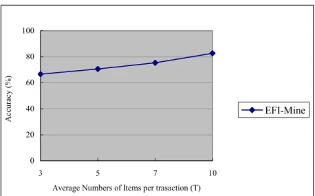
Effects of Varying Transaction Size
We investigate the effects of varying transaction size on the accuracy of mining results i.e., the average number of items per transaction. As shown in Figure 2-10, if T is larger, the accuracy is higher than under T. This is because T can bring more information and trend from past transactions. This indicates that EFI-Mine fits for mining temporal databases with large transaction size. 0 20 40 60 80 100 3 5 7 10
Average Numbers of Items per trasaction (T)
A ccur acy ( % ) EFI-Mine
Effects of Varying Number of Items
In this last experiment, we investigate the effects of varying the numbers of items on the accuracy of mining results. The results are as shown in Figure 2-11. We observe that the accuracy decreases when the numbers of items are increased. This is because too many items will affect the stability of the patterns. On the contrary, the accuracy under smaller numbers of items could reach almost 100%. This indicates that EFI-Mine fits for mining temporal databases with small numbers of items.
0 20 40 60 80 100 50 100 200 300 Numbers of Items (N) A ccur acy ( % ) EFI-Mine
Chapter 3
Mining Temporal High Utility Itemsets from
Temporal Databases
3.1 Problem Definition
The mining of association rules for finding the relationship between data items in large databases is a well studied technique in the data mining field with representative methods like
Apriori [1][2]. The problem of mining association rules can be decomposed into two steps.
The first step involves finding of all frequent itemsets (or say large itemsets) in databases. Once the frequent itemsets are found, generating association rules is straightforward and can be accomplished in linear time.
An important research issue extended from the mining of association rules is the discovery of temporal association patterns in temporal databases due to the wide applications on various domains. Temporal data mining can be defined as the activity of discovering interesting correlations or patterns in large sets of temporal data accumulated for other purposes [6]. For a database with a specified transaction window size, we may use an algorithm like Apriori to obtain frequent itemsets from the database. For time-variant temporal databases, there is a strong demand to develop an efficient and effective method to mine various temporal patterns [13]. However, most methods designed for traditional databases cannot be directly applied to the mining of temporal patterns in temporal databases because of their high complexity.
recent data in temporal databases. That is, in temporal data mining, one should not only include new data (i.e., data in the new hour) but also remove the old data (i.e., data in the most obsolete hour) from the mining process. Without loss of generality, consider a typical market-basket application as illustrated in Figure 3-1, where the transactional data of customer purchases are shown as time advances.
Figure 3-1. An example of online transaction flows.
In Figure 3-1, for example, data was accumulated as a function of time. Data obtained prior to some specified time interval in the past becomes useless for reference. People might be most interested in the temporal association patterns in the latest three hours (i.e., db3,5) as shown in Figure 3-1. It can be seen that in such a temporal database environment it is intrinsically difficult to conduct the frequent pattern identification due to the constraints of limited time and memory space. Furthermore, it takes considerable time to find temporal frequent itemsets in different time windows. However, the frequency of an itemset may not be a sufficient indicator of interestingness, because it only reflects the number of transactions in the database that contain the itemset. It does not reveal the utility of an itemset, which can be measured in terms of cost, profit or other expressions of user preferences. On the other hand, frequent itemsets may only contribute a small portion of the overall profit, whereas
non-frequent itemsets may contribute a large portion of the profit. In reality, a retail business may be interested in identifying its most valuable customers (customers who contribute a major fraction of the profits to the company). Hence, frequency is not sufficient to answer questions such as whether an itemset is highly profitable, or whether an itemset has a strong impact. Utility mining is thus useful in a wide range of practical applications and was recently studied in [8][21][35]. This also motivates our research in developing a new scheme for finding temporal high utility itemsets (THUI) from temporal databases.
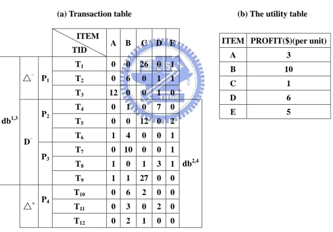
Table 3-1. A transaction database and its utility table.
(a) Transaction table (b) The utility table ITEM TID A B C D E T1 0 0 26 0 1 T2 0 6 0 1 1 △一 P1 T3 12 0 0 1 0 T4 0 1 0 7 0 T5 0 0 12 0 2 P2 T6 1 4 0 0 1 T7 0 10 0 0 1 T8 1 0 1 3 1 db1,3 D一 P3 T9 1 1 27 0 0 T10 0 6 2 0 0 T11 0 3 0 2 0 △+ P4 T12 0 2 1 0 0 db2,4
ITEM PROFIT($)(per unit) A 3 B 10 C 1 D 6 E 5
Recently, a utility mining model was defined in [35]. Utility is considered as a measure of how “useful” (e.g., “profitable”) an itemset is. The definition of utility u(X) of an itemset X is the sum of the utilities of X in all transactions containing X. The goal of utility mining is to identify high utility itemsets which drive a large portion of the total utility. Traditional
association rules mining models assume that the utility of each item is always 1 and the sales quantity is either 0 or 1, thus it is only a special case of utility mining, where the utility or the sales quantity of each item could be any number. If u(X) is greater than a utility threshold, X is a high utility itemset. Otherwise, it is a low utility itemset. Table 3-1 is an example of utility mining in a transaction database. The number in each transaction in Table 3-1(a) is the sales volume of each item, and the utility of each item is listed in Table 3-1(b). For example, u({B, D}) = (6×10+1×6) + (1×10+7×6) + (3×10+2×6) = 160. {B, D} is considered as a high utility itemset if the utility threshold is set at 120.
However, a high utility itemset may consist of some low utility items. Another attempt is to adopt the level-wise searching schema that exists in fast algorithms such as Apriori [3]. However, this algorithm does not apply to the utility mining model. For example, consider u(D) = 84 < 120 as shown in Table 3-1, D is a low utility item. However, its superset {B, D} is a high utility itemset. If Apriori is used to find high utility itemsets, all combinations of the items must be generated. Moreover, the number of candidates is prohibitively large in discovering a long pattern. The cost of either computation time or memory will be intolerable, regardless of what implementation is applied. The challenge of utility mining is not only in restricting the size of the candidate set but also in simplifying the computation for calculating the utility. Another challenge of utility mining is how to find temporal high utility itemsets from temporal databases as time advances.
In this chapter, we explore the issue of efficiently mining high utility itemsets in temporal databases like data streams. We propose an algorithm named THUI-Mine that can discover temporal high utility itemsets from temporal databases efficiently and effectively. The underlying idea of THUI-Mine algorithm is to integrate the advantages of Two-Phase algorithm [21] and SWF algorithm [18] with augmentation of the incremental mining techniques for mining temporal high utility itemsets efficiently. The novel contribution of
THUI-Mine is that it can efficiently identify the utility itemsets in temporal databases so that
THUI-Mine can discover the temporal high utility itemsets in current time window and also
discover the temporal high utility itemsets in the next time window with limited memory space and less computation time by sliding window filter method. In this way, the process of discovering all temporal high utility itemsets under all time windows of temporal databases can be achieved effectively under less memory space and execution time. This meets the critical requirements of time and space efficiency for mining temporal databases. Through experimental evaluation, THUI-Mine is shown to produce fewer candidate itemsets in finding the temporal high utility itemsets, so it outperforms other methods in terms of execution efficiency. It is observed that the average improvement of THUI-Mine over Two-Phase algorithm reaches to about 67%. Moreover, it also achieves high scalability in dealing with large databases. To our best knowledge, this is the first work on mining temporal high utility itemsets from temporal databases.
The rest of this chapter is organized as follows: Section 3.2 describes the proposed approach, THUI-Mine, for finding the temporal high utility itemsets. In section 3.3, we describe the experimental results for evaluating the proposed method. The conclusion of the chapter is provided in Section 3.4.
3.2 Proposed Method
In this section, we present the THUI-Mine method. We describe the basic concept of
THUI-Mine and give an example for mining temporal high utility itemsets. The procedure of
the THUI-Mine algorithm is provided in the last paragraph the section.
Basic Concept of THUI-MINE
The goal of utility mining is to discover all the itemsets whose utility values are beyond a user specified threshold in a transaction database. In [35], the goal of utility mining is defined as
the discovery of all high utility itemsets. An itemset X is a high utility itemset if u(X) ≥ε, where X I and ε is the minimum utility threshold; otherwise, it is a low utility itemset. For example, in Table 3-1, u(A, T
⊆
8) = 1×3 = 3, u({A, C}, T8) = u(A, T8) + u(C, T8) = 1×3 + 1×1 =
4, and u({A, C}) = u({A, C}, T8) + u({A, C}, T9) = 4 + 30 = 34. If ε = 120, {A, C} is a low
utility itemset. However, if an item is a low utility item, its superset may be a high utility itemset. For example, consider u(D) = 84 < 120, D is a low utility item, but its superset {B, D} is a high utility itemset since u({B, D}) = 160 > 120. Intuitively, all combinations of items should be processed so that it never loses any high utility itemset. However, this will incur intolerable cost on computation time and memory space. A set of terms leading to the formal definition of utility mining problem can be generally defined as follows by referring to [35]:
z I = {i1, i2, …, im} is a set of items.
z D = {T1, T2, …, Tn} is a transaction database where each transaction Ti∈D is a subset of I.
z o(ip, Tq), local transaction utility value, represents the quantity of item ip in transaction Tq. For example, o(A, T3) = 12, as shown in Table 3-1(a).
z s(ip), external utility, is the value associated with item ip in the Utility Table. This value
reflects the importance of an item, which is independent of transactions. For example, in Table 3-1(b), the external utility of item A, s(A), is 3.
z u(ip, Tq), utility, the quantitative measure of utility for item ip in transaction Tq, is defined
as o(ip, Tq)×s(ip). For example, u(A, T3) = 12 × 3, in Table 3-1.
z u(X, Tq), utility of an itemset X in transaction Tq, is defined as , where X =
{ i
∑
∈X ip q p T i u( , ) 1, i2, …, im} is a k-itemset, X ⊆ Tq and 1≤ k≤ m.z u(X), utility of an itemset X, is defined as
∑
⊆ ∧ ∈ q q q T X D T T X u( , ).
Liu et al. [21] proposed the Two-Phase algorithm for pruning candidate itemsets and simplifying the calculation of utility. First, the Phase I overestimates some low utility itemsets,
but it never underestimates any itemsets. For the example in Table 3-1, the transaction utility
of transaction Tq, denoted as tu(Tq), is the sum of the utilities of all items in Tq: tu(Tq) = . Moreover, the transaction-weighted utilization of an itemset X, denoted as twu(X),
is the sum of the transaction utilities of all the transactions containing X: twu(X) = For example, twu(A) = tu(T
∑
∈ q p q p T i T i u( , )∑
∈ ⊆T D X q q T tu( ).3) + tu(T6) + tu(T8) + tu(T9) = 42 + 48 + 27 + 40 = 157 and twu({D,
E}) = tu(T2) + tu(T8) = 71 + 27 = 98. In fact, u(A) = u({A}, T3) + u({A}, T6) + u({A}, T8)+
u({A}, T9)=36 + 3 + 3 + 3 = 45 and u({D, E}) = u({D, E}, T2) + u({D, E}, T8)= 11 + 23 = 34.
Table 3-2 gives the transaction utility for each transaction in Table 3-1. Second, one extra database scan is performed to filter the overestimated itemsets in phase II. For example, by observing that twu(A) = 157 > 120 and u(A) = 45 < 120, the item {A} is pruned. Otherwise, it is a high utility itemset. Finally, all high utility itemsets are discovered in this way.
We illustrate the detail process of Two-Phase algorithm by the following example in db1,3 of Table 3-1. Suppose the utility threshold is set as 120 with nine transactions in db1,3. In Phase I, the high transaction-weighted utilization 1-itemsets {A, B, C, D, E} are generated since twu(A) = tu(T3) + tu(T6) + tu(T8) + tu(T9) = 42 + 48 + 27 + 40 = 157 > 120, twu(B) =
tu(T2) + tu(T4) + tu(T6) + tu(T7) + tu(T9) = 71 + 52 + 48 + 105 + 40 = 361 > 120, twu(D) =
tu(T2) + tu(T3) + tu(T4) + tu(T8) = 71 + 42 + 52 + 27 = 192 > 120 and twu(E) = tu(T1) + tu(T2)
+ tu(T5) + tu(T6) + tu(T7) + tu(T8) = 31 + 71 + 22 + 48 + 105 + 27 = 304 > 120. Then, 10
candidate 2-itemsets {AB, AC, AD AE, BC, BD, BE, CD, CE, DE} are generated by the high transaction-weighted utilization 1-itemsets {A, B, C, D, E} in the first database scan. In the same way, the high transaction-weighted utilization 2-itemset {BE} are generated since
twu(AB) = tu(T6) + tu(T9) = 48 + 40 = 88 < 120, twu(AC) = tu(T8) + tu(T9) = 27 + 40 = 67 <
120, twu(AD) = tu(T3) + tu(T8) = 42 + 27 = 69 < 120, twu(AE) = tu(T6) + tu(T8) = 48 + 27 =
75 < 120, twu(BC) = tu(T9) = 40 < 120, twu(BD) = tu(T4) = 52 < 120, twu(BE) = tu(T2) +