Plant uncertainty analysis in a duct active noise control
problem by using the H
`theory
Mingsian R. Bai and Hsinhong Lin
Department of Mechanical Engineering, Chiao-Tung University, 1001 Ta-Hsueh Road, Hsin-Chu 30050, Taiwan, Republic of China
~Received 2 June 1997; accepted for publication 25 March 1998!
Plant uncertainty is one of the major contributing factors that could affect the performance as well as stability of active noise control ~ANC! systems. Plant uncertainty may be caused by either the errors in modeling, computation, and measurement, or the perturbations in physical conditions. These factors lead to deviations of the plant from the nominal model, which will in turn affect the robustness of the control system. In this paper, the effects due to changes in physical conditions on the ANC system are investigated. The analysis is carried out in terms of performance and robustness by using a general framework of the H` robust control theory. The size of plant uncertainty is estimated according to the infinity norm of the perturbations to physical conditions, which provides useful information for subsequent controller design that accommodates both performance and stability in an optimal and robust manner. The guidelines for designing the ANC systems with reference to plant uncertainties are also addressed. © 1998 Acoustical Society of America.
@S0001-4966~98!02007-4#
PACS numbers: 43.50.Ki@GAD#
INTRODUCTION
Active noise control ~ANC! has received persistent re-search attention since Lueg filed his patent.1 Advances in fundamental theories, control algorithms, and practical appli-cations of the ANC field have been achieved and can be found in much literature, e.g., Refs. 2 and 3. The potential of this emerging technology masks somewhat the limitations that prevent the technology from full commercial use. One of the limitations of the ANC techniques is the robustness prob-lem of the control systems in the face of plant uncertainties. Plant uncertainties influence the performance and even the stability of closed-loop feedback control systems so severe that ANC methods are sometimes viewed as unreliable ap-proaches in comparison with conventional passive means.
Plant uncertainties generally arise because of the errors in modeling, computation, and measurement. In addition, plant uncertainties may be caused by the change of environ-mental factors. For example, modeling errors are inevitable prior to an ANC design of a low-frequency duct silencer, where high-frequency modes are usually truncated so that a controller of reasonable order can be implemented. Aside from the modeling error, perturbations of the duct system may also occur due to variations of physical conditions, e.g., temperature, viscosity, boundary conditions, and so forth. In this sense, plant uncertainties are referred to as the plant
variations due to changes in physical conditions. These
fac-tors result in deviations of the plant from the nominal model, which in turn affects the robustness of the closed-loop sys-tem. A good feedback ANC system needs a reasonably ac-curate nominal model for the acoustic plant, which is is as-sumed to be linear time-invariant ~LTI!. In many control problems encountered in ANC applications, plant uncertain-ties can be so severe that any attempt to employ stable feed-back controllers results in unacceptable performance.
In this paper, the effects due to changes in physical con-ditions on the ANC duct silencer are investigated. With the change of various physical conditions taken into account, the mathematical model of a low-frequency duct is established. Performance and robustness analysis is then carried out by using a general framework of the H` robust control theory.4–9 The size of plant uncertainty is first estimated ac-cording to the infinity norm of the perturbations to various physical conditions. This provides useful information in choosing appropriate weighting functions for designing an optimal feedback controller that accommodates both perfor-mance and stability in a robust manner. The guidelines for designing the ANC systems with reference to plant uncer-tainties are also addressed. It should also be remarked that the discussions of this paper are limited to fixed, feedback systems only. The results do not always apply to other ANC methods such as feedforward structures.
I. MATHEMATICAL MODELING OF THE LOW-FREQUENCY DUCT
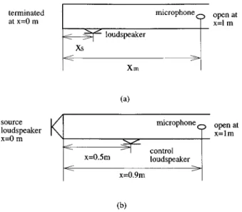
In this section, the mathematical models of the sound fields in a rectangular duct subject to various physical con-ditions are derived. A duct of length l is schematically shown in Fig. 1~a!. It is assumed that the duct is open at one end and terminated at the other. Below the cutoff frequency, the sound field in the duct can be treated as one dimensional with spatial coordinate x, 0<x<l. A monopole source is located at x5xs, while the sensor is located at x5xm.
To begin with, we consider the joint effects due to lin-ing, viscosity, temperature, and flow. Knowing that, similar to the loss mechanism due to viscosity of the medium, the effect of duct lining is to dissipate acoustic energy at the boundaries. As shown in pp. 26–30 of Ref. 12, lining duct walls results in attenuations in the axial direction and the
plane-wave number becomes complex. By the same token, rather than modeling the duct lining precisely as a boundary condition, we take a simpler approach to model this attenu-ation effect by an ad hoc relaxattenu-ation constantt, which corre-sponds to the complex wave number
k5v c
1
A
11 jvt, ~1!where v is angular frequency and c is sound speed.10 By substituting the definition
k[b2 ja ~2!
into Eq. ~1! and by collecting real and imaginary parts, the attenuation constant ais obtained
a5 k &
@
A
11~vt!221#1/2. ~3!In the following simulation, the attenuation constant a, or equivalently the relaxation constant t, for each case can be obtained from the method described in p. 510 of Ref. 11. Following the procedure described in pp. 503–510 of Ref. 11, we further assume the normal acoustical impedance of the lining to be Z5 f 3(0.4712 j0.392), where f is the fre-quency in Hz.
Next the temperature is assumed for simplicity to be uniformly distributed inside the duct. Therefore the effect of temperature variation would be to alter the speed of sound.10 That is,
c5C0
A
11 T273, ~4!
where C0 is sound speed at 0 °C and T is Celsius
tempera-ture.
It can be shown that the dynamic equation that incorpo-rates the effects due to lining, viscosity, temperature, and flow for the sound field in the duct is12
S
11t ] ]tD
¹ 2p~x,t!51 c D2 Dt2 p~x,t!1d~x,t! ~5!with the material derivative
D Dt[ ] ]t1u ] ]x,
where u is mean flow velocity, p is the sound pressure, and r0 is the density of acoustic medium. It is assumed that a
monopole source13 is located at x5xs.
d~x,t!5vs~t!d~x2xs!, ~6!
where vs is the volume velocity. Assume further that the boundary conditions of the duct are
] ]x p~0,t!50 at x50 ~7! and p~l,t!50 at x5l. ~8! By separation of variables p~x,t!5q~t!v~x!, ~9!
Eq. ~5! can be written into a modal form
q¨~t!1Viq˙i~t!1
(
j51 jÞi ` vi jq˙j~t!1ciq˙i~t!1liqi~t!5bius~t!, ~10! where bi[ni~xs!, u~t![r0v~t!, Vi5 u l @~21! i21#, vi j5 ~2 j21!p lF
cos@~i1 j21!p#21 i1 j21 1cos@~ j2i!j2ip#21G
, ~11! ci5c~T!2tiF
~2i21!p lG
2 , li5~c 22u2!F
~2i21!p lG
2 , with ni~x!5c~T!A
2 l cos ~2i21!p 2l x. ~12!Hence the sound pressure ym measured by a microphone located at x5xmis
ym~t!5p~xm,t!5
(
j51`
qj~t!vj~xm!. ~13!
To obtain the state-space model, we retain only r modes and let
FIG. 1. ~a! Modeling configuration of the low-frequency duct; ~b! the ex-perimental configuration of the low-frequency duct.
x~t!5@q1 q1 ¯ qr qr#, y~t!5ym~t! so that x˙~t!5Ax~t!1Bus~t!, y~t!5Cx~t!, ~14! where Ai j5
5
i is odd:H
j5i11: Ai j51 others: Ai j50 i is even:H
j5i: Ai j5Vi/2 j5i21: Ai j5li/2 others:H
j is odd: Ai j50 j is even: Ai j5vi/2j/2 , B5@0 b1 ¯ 0 br#T, C5@V1~xm! 0 ¯ Vr~xm! 0#.The second half of the section is focused on the model-ing of the sound field in the duct subject to the radiation impedance at the open end. This boundary condition can be described by an impedance function14
Zl~s!5 p~l,s!
u~l,s!, x5l, ~15!
where Zl(s) is the Laplace transform of the specific acoustic impedance. The relationship between the sound pressure and the particle velocity satisfies the momentum equation
]p~x,s!
]x 52r0su~l,s!. ~16!
Thus the problem is formulated as the following modified wave equation and boundary conditions:
1 c~T!2
S
s 212us ] ]x1u 2 ] 2 ]x2D
p~x,s! 5~11ts! ] 2 ]x2 p~x,s!1r0svs~s!d~x2xs! such that ]p~0,s! ]x 50, ~17! p~l,s!52 1 sr0 Zl~s! ]p~l,s! ]x ,where c(T) is the speed of sound as a function of tempera-ture T. It can be shown by some manipulations that the trans-fer function between any source point and field point is15
G~x,j,s!5
5
x,j c~T!2~l2el2x2l1el1x!@el2~12j!2el1~12j!1~Zl/sr0!~l2el2~12j!2l1el1~12j!!# e~l11l2!x~l 22l1!@u22~11ts!c~T!2#@l2el12l1el21~Zl/sr0!l1l2~el12el2!# x.j c~T!2~l2el1j2l1el2j!@el11l2x2el21l1x1~Zl/sr0!~l1el11l2x2l2el21l1x!# e~l11l2!j~l 22l1!@u 22~11ts!c~T!2#@l 2el12l1el21~Zl/sr0!l1l2~el12el2!# ,wherel1(s) andl2(s) are two roofs of
l22 2us
u22~11ts!c~T!2 l2
s2
u22~11ts!c~T!250. ~18!
In terms of G(x,j,s), the Laplace transform of sound pres-sure at any location x in the duct can be expressed as
p~x,s!5G~x,j,s!uj5x
sQ~xs,s!, ~19!
where Q(xs,s) is the Laplace transform ofr0v˙s(t). It should be noted that the above solution gives an exact description of the system without truncating any high-order terms. Thus Eq.~18! can be used to calculate the frequency response and provides complete information about plant uncertainties. However, it is generally difficult to produce dynamic re-sponses, as required in a numerical simulation, based on Eq.
~18! that are not a rational transfer function. To obviate the
problem, we simply curve-fit the frequency response of Eq.
~18! and convert it into a more tractable rational transfer
function by using aMATLABroutineINVFREQS.16
II.H` ROBUST CONTROL ANALYSIS AND
SYNTHESIS
A brief review of the H` robust control theory is given in this section. Because the H` theories can be found in much control literature,4–9 we present only the key ones needed in the analysis of our problem. The rest are men-tioned without proof.
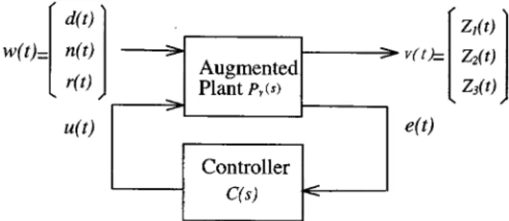
In modern control theory, all control structures can be described by using a generalized control framework, as de-picted in Fig. 2. The framework contains a controller C(s) and an augmented plant Pg(s). The controlled variablen(t) corresponds to various control objectives z1(t), z2(t), and
z3(t), and the extraneous input w(t) consists of the reference
r(t), the disturbance d(t), and the noise n(t). The signals u(t) and e(t) are the control inputs to the plant and the
measured output from the plant, respectively. The general input–output relation can be expressed as
Pg~s!5
F
P11~s! P12~s! P21~s! P22~s!
G
, ~20!
par-titions of the augmented plant Pg(s) and the symbols are capitalized to represent the Laplace transform variables. The main idea of the H`control is to minimize the infinity norm of the transfer function Tnw(s) between n(t) and w(t) that can be expressed by the linear fraction transformation~LFT!
Tnw~s!5LFT„Pg~s!,C~s!…
5P11~s!1P12~s!C~s!@12P22~s!C~s!#21P21~s!. ~21!
Hence the optimal H`problem can be stated as min
C~s!iTnw~s!i`5minC~s! sup
2`<v<`iTnw~ jv!i. ~22! However, instead of finding the optimal solution, which is generally very difficult, one is content with the suboptimal solution that can be analytically obtained. This becomes the
so-called standard H` problem: finding C(s) such that iTnw(s)i`,1.
Insofar as the solution of the suboptimal problem is con-cerned, we would like to remark that the H` algorithms are by large divided into two classes: the model matching algo-rithms ~the 1984 approach! and the two Riccati equation al-gorithms ~the 1988 approach!. The details are omitted for brevity. The interested reader may consult Refs. 4 and 7.
In the sequel, an analysis is carried out for the feedback structure ~Fig. 3! on the basis of the generalized control framework. The symbols P1(s) and P2(s) correspond to the
primary ~disturbance! path and the secondary ~control! path, respectively. To find an H`controller, we weight the sensi-tivity function S˜ (s) by W1(s), the control input u(t) by W2(s), and the complementary sensitivity function T˜ (s) by
W1(s), where the sensitivity function and the complemen-tary sensitivity function are defined, respectively, as17
S ˜ ~s!511P 1 2~s!C~s! ~23! and T ˜ ~s!5 P2~s!C~s! 11P2~s!C~s! . ~24!
Note that S˜ (s)1T˜(s)51. To achieve disturbance rejection and tracking performance, the following nominal perfor-mance condition must be satisfied
iS˜~s!W1~s!i`,1. ~25!
FIG. 3. System diagrams of the active silencer diagrams.~a! Duct arrangement; ~b! block diagram of the feedback control. FIG. 2. Generalized control framework. Pg(s) is the augmented plant and
On the other hand, for system stability against plant pertur-bations and model uncertainties, the robustness condition de-rived from the small-gain theorem7 must also be satisfied
iT˜~s!W3~s!i`,1. ~26!
The choice of W3(s) is determined by the size of uncertainty D that is defined in
P ˜
25~11D!P2, ~27!
where P2 and P˜2 are the nominal and the perturbed plants,
respectively. The idea behind this definition of uncertainty is that D is the plant perturbation away from the nominal one and souD( jv)u provides the uncertainty profile and the peak of which~evaluated by the infinity norm! renders the size of uncertainty.
In the common practice of loop shaping, W1(s) is
cho-sen as a low-pass function and W3(s) is chosen as a
high-pass function. The guidelines for choosing weight functions can be found in pp. 255–268 of Ref. 8. It is well known that the trade-off between S˜ (s) and T˜(s) in conjunction with the
waterbed effect dictate the performance and robustness of the
feedback design. This classical trade-off renders the so-called mixed sensitivity problem:8
iuS˜~s!W1~s!u1uT˜~s!W3~s!ui`,1 ~28!
which is also a necessary and sufficient condition for the controller to achieve robust performance.
In terms of the generalized control framework, the input–output relation of the augmented plant corresponding to the feedback structure is
F
Z1~s! Z2~s! Z3~s! E~s!G
5F
W1~s! 2W1~s!P2~s! 0 W2~s! 0 W3~s!P2~s! 1 2P2~s!G
F
D~s! U~s!G
. ~29!Hence it can be shown by LFT that the suboptimal condition of the feedback controller is
I
F
W1~s!S˜~s! W2~s!S˜~s!C~s! W3~s!T˜~s!G
I
`,1. ~30!
III. NUMERICAL SIMULATION
Numerical investigations were carried out to explore the characteristics of the forgoing H`-based active controller subject to various plant perturbations. In the simulation, a rectangular duct with 0.2530.25-m cross section ~cutoff frequency5690 Hz! and of length 1 m is selected. A mono-pole source is located at one end of the duct, while the duct is left open at the other end@Fig. 1~b!#. Another loudspeaker located at x50.5 m is used as the actuator. The sensor is
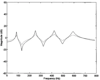
FIG. 4. Frequency response of the derived model and a real muffler~derived model: ———; real muffler: ---!. ~a! Magnitude ~dB!; ~b! Phase ~degree!. TABLE I. The mathematical models of the sound field in the duct subject to
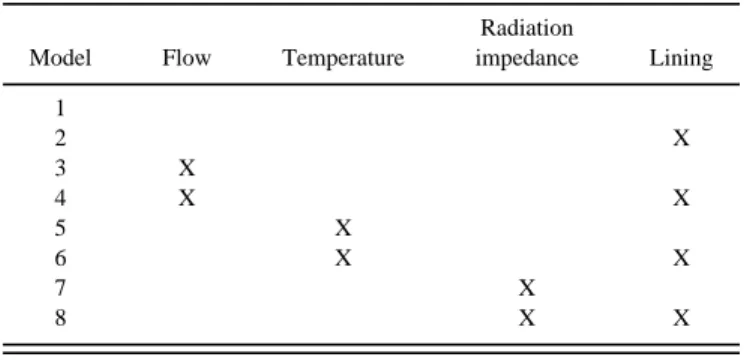
different physical conditions.
Model Flow Temperature
Radiation impedance Lining 1 2 X 3 X 4 X X 5 X 6 X X 7 X 8 X X
TABLE II. The system poles and zeros of model 1. The asterisk denotes nonminimal phase zeros.
Primary path Secondary path
Zeros (3103) Poles (3103) Zeros (3103) Poles (3103)
*2.272561.5081i 20.000560.5341i *1.856461.3748i 20.000560.5341i
20.000463.5118i 20.000561.6022i 20.000563.4732i 20.000561.6022i 22.273161.5076i 20.000562.6703i 21.857361.3742i 20.000562.6703i 20.000563.7384i 20.000563.7384i
gain522.7876 gain55.5771
TABLE III. The system poles and zeros of model 2. The asterisk denotes nonminimal phase zeros.
Primary path Secondary path
Zeros (3103) Poles (3103) Zeros (3103) Poles (3103)
*2.259961.5705i 20.020260.5336i *1.840361.4189i 20.020260.5336i
20.109463.5101i 20.041261.6017i 20.107463.4716i 20.041261.6017i 22.284861.4459i 20.067562.6695i 21.872661.3305i 20.067562.6695i 20.125363.7364i 20.125363.7364I
gain522.7876 gain55.5771
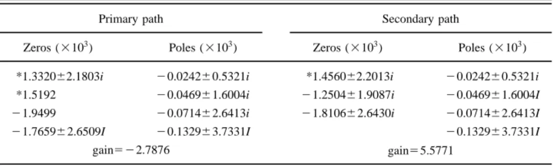
TABLE IV. The system poles and zeros of model 3. The asterisk denotes nonminimal phase zeros.
Primary path Secondary path
Zeros (3103) Poles (3103) Zeros (3103) Poles (3103)
*1.442362.5471i 20.021660.5332i *1.332062.1803i 20.024260.5299i
*1.5192 20.027661.6020i 20.416463.0452i 20.027661.5902i
21.9499 20.032162.6678i 21.765962.6509i 20.032162.6510i 22.756962.7680i 20.046363.7372i 20.046363.7577i
gain522.7876 gain55.5771
TABLE V. The system poles and zeros of model 4. The asterisk denotes nonminimal phase zeros.
Primary path Secondary path
Zeros (3103) Poles (3103) Zeros (3103) Poles (3103)
*1.332062.1803i 20.024260.5321i *1.456062.2013i 20.024260.5321i
*1.5192 20.046961.6004i 21.250461.9087i 20.046961.6004I
21.9499 20.071462.6413i 21.810662.6430i 20.071462.6413I 21.765962.6509I 20.132963.7331I 20.132963.7331I
located at x50.9 m. In what follows, a series of numerical experiments will be conducted to explore the effects of flow, temperature, and radiation impedance on the system. To aid the comparison, the models used in the simulation under various physical conditions are summarized in Table I.
To show how well the derived model matches a real duct silencer, the frequency response magnitude and phase of model 2 is compared with a real silencer with lining in p. 27 of Ref. 12. The comparison shown in Fig. 4 indicates that the derived model agrees reasonably well with a real silencer.
In the first experiment, the effect of flow on the duct silencer is examined. In addition, it is demonstrated in this experiment that the size of uncertainty due to flow relies on whether the duct is lined or not. In the lined duct, the walls of the duct are lined with absorbing material. The lining thickness and the flow resistance of the absorptive lining material are 0.025 m and 4000 mks rayls, respectively. The cross section of the lined duct is intentionally chosen to be the cross section of a duct in p. 503 of Ref. 11. Using the mathematical model derived in the last sections, the system poles and zeros of the unlined duct and the lined duct for the
stationary medium ~models 1 and 2 in Table I! are listed in Tables II and III, respectively. The system poles and zeros of the unlined duct and the lined duct for the moving medium
~mean flow velocity530 m/s; models 3 and 4 in Table I! are
listed in Tables IV and V, respectively. Before showing the result, a brief note regarding duct lining is in order. The importance of passive lining that has often been overlooked in ANC design lies in not only high-frequency attenuation but also the robustness of active control with respect to plant uncertainties.18With proper damping treatment, the plant can be gain-stabilized even when the flexible modes are poorly modeled. Another benefit of passive lining is that a lower order of plant model can usually be obtained than the lightly damped plants so that numerical error is reduced. The impor-tance of passive treatment can be seen by noting the effect of flow subject to different lining conditions. By comparing the nominal model 1 and the perturbed model 3, the plant uncer-tainty due to flow calculated for the unlined duct is shown by a solid line in Fig. 5. Similarly, by comparing the nominal model 2 and the perturbed model 4, the plant uncertainty due to flow calculated for the lined duct is shown by a dashed line in the same figure. The peaks of uncertainty appear at the resonances and antiresonances of the nominal perturbed plants. However, as seen in Fig. 5, the peaks of the lined duct are lower than those of the unlined duct. This implies that the passive lining indeed has the desirable effect of neutralizing system perturbation. The smaller the size of uncertainty is, the less the requirement of robust stability and the more room for achieving performance in the control design. On the basis of the plant uncertainty due to flow, optimal con-trollers can be obtained for both the unlined duct and the lined duct by using the aforementioned H`design procedure
~Fig. 6!. The resulting loop shaping of sensitivity functions
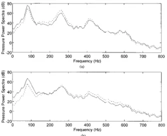
versus weight functions for the unlined duct and the lined duct are shown in Figs. 7 and 8. The active control results in terms of the power spectrum of sound pressure at the sensor position are shown in Fig. 9. It can be observed that the performance of the lined duct is better than the unlined duct
~12 dB versus 7 dB at the peak of 85 Hz! and also the
effective control band of the lined duct is wider than the
FIG. 5. Plant uncertainty due to moving medium~mean-flow velocity530 m/s!. Without lining: ———; with lining: ---.
FIG. 6. Magnitude ~dB! of frequency responses of the H` controllers
~mean-flow velocity530 m/s!. ~a! Unlined duct; ~b! lined duct.
FIG. 7. Loop shaping for the unlined duct~mean-flow velocity530 m/s!. ~a!
control band of the unlined duct. It is noteworthy that Fig. 9 shows good control at low frequency down to 0 Hz because the acoustic sources used in the simulation are ideal point sources. Practical acoustic actuators should have poor re-sponse at the very low-frequency range.
In the second experiment, the effect of temperature variation on the silencer is examined. It is assumed that the temperature is changed from 25 to 90 °C for both the unlined duct and the lined duct. By comparing the nominal model 1 and the perturbed model 5, the plant uncertainty due to tem-perature variation calculated for the unlined duct is shown by a solid line in Fig. 10. Similarly, by comparing the nominal model 2 and the perturbed model 6, the plant uncertainty due to flow calculated for the lined duct is shown by a dashed line in the same figure. The plant uncertainty shows strong peaks~maximum 45 dB! for the unlined duct, while the plant uncertainty of the lined duct shows only moderate variations. This sharp contrast~which is even more pronounced than the forgoing case of flow effect! indicates again the need of pas-sive lining, insofar as the system robustness against system
perturbation is concerned. In fact, for the unlined duct, the plant uncertainty is so severe that virtually no controller can meet the requirements of the H` design. Hence only the controller for the lined duct is calculated on the basis of the plant uncertainty. For brevity, we omit the frequency re-sponse of the controller and show only the result of active control in Fig. 11. Noise attenuation is achieved by using the lined duct in the band 0–150 Hz. Nevertheless, noise ampli-fication around the second peak at 280 Hz indicates the dif-ficulty in designing the controller to accommodate the per-turbation due to temperature variation.
In the third experiment, the effect of radiation imped-ance at the open end of the duct is examined. The Laplace transform of radiation impedance is assumed to be Zt 520.01s21100s that is intentionally made larger than that
of an open end. This situation may happen, for example, when the open end of the silencer is near a wall. Because the importance of passive lining against plant uncertainty has been manifested in the previous cases, we now explore the effect of radiation impedance on only the lined duct. Taking model 2 as the nominal case and model 8 as the perturbed case, the corresponding plant uncertainty is shown in Fig. 12.
FIG. 8. Loop shaping for the lined duct~mean-flow velocity530 m/s!. ~a!
W121(s):¯ versus S˜(s): ———; ~b! W321(s):¯ versus T˜ (s): ———.
FIG. 9. The active control results for the duct subject to flow effect in terms of the power spectrum of sound pressure at the sensor position~control off: ———; control on: ---!. ~a! Without lining; ~b! with lining.
FIG. 10. Plant uncertainty due to temperature variation~25–90 °C!. Without lining: ———; with lining: ---.
FIG. 11. The active control results for the lined duct subject to temperature variation in terms of the power spectrum of sound pressure at the sensor position~control off: ———; control on: ---!.
TABLE VI. The system poles and zeros of model 5. The asterisk denotes nonminimal phase zeros.
Primary path Secondary path
Zeros (3103) Poles (3103) Zeros (3103) Poles (3103)
*1.511462.4650i 20.000560.5950i 1.487662.5214i 0.000560.5950i
*1.7214 20.000560.7851i 1.239063.7165i 0.000561.7851i
22.1520 20.000562.9752i 1.941662.9247i 0.000562.9752i
21.945362.9362i 20.000564.1653i 0.000564.1653i gain522.7876 gain55.5771
TABLE VII. The system poles and zeros of model 6. The asterisk denotes nonminimal phase zeros.
Primary path Secondary path
Zeros (3103) Poles (3103) Zeros (3103) Poles (3103)
*1.511462.4650i 20.020260.5950i *1.489262.4319i 20.020260.5950i
21.721462.1520i 20.041261.7851i 21.675462.2347i 20.041261.7851i 21.945362.9362i 20.067562.9752i 21.889262.8764i 20.067562.9752i 20.125364.1653i 20.125364.1653i
gain522.7876 gain55.5771
TABLE VIII. The system poles and zeros of model 7. The asterisk denotes nonminimal phase zeros.
Primary path Secondary path
Zeros (3103) Poles (3103) Zeros (3103) Poles (3103)
*1.676362.5082i 20.000560.5162i *1.604362.5732i 20.000560.5162i
*1.4182 20.000561.5486i 21.143262.1746i 20.000561.5486i
21.8490 20.000562.5811i 21.222662.0457i 20.000562.5811i 21.242562.0380i 20.000563.6135i 20.000563.6135i
gain522.7876 gain55.5771
TABLE IX. The system poles and zeros of model 8. The asterisk denotes nonminimal phase zeros.
Primary path Secondary path
Zeros (3103) Poles (3103) Zeros (3103) Poles (3103)
*1.211361.9981i 20.020260.5158i *1.214561.9972i 20.020260.5158i
*1.3855 20.041261.5451i *1.4255 20.041261.5451i
21.8884 20.067562.5784i 21.8912 20.067562.5784i 21.211361.9981I 20.125363.6012i 21.231861.9847I 20.125363.6012i
The plant uncertainty due to radiation impedance appears less drastic than the temperature effect. On the basis of the plant uncertainty, optimal controllers are obtained for the lined duct by using the H` design procedure. The resulting loop shaping of sensitivity functions versus weight functions is shown in Fig. 13. The active control results in terms of the power spectrum of sound pressure at the sensor position are shown in Fig. 14. It can be observed that the effective control bandwidth is approximately 140 Hz and the first peak of sound pressure at 82 Hz is attenuated by approximately 15 dB. The poles and zeros of models 5–8 are shown in Table VI–IX.
In the last experiment, the effect of time delay is inves-tigated. The microphone is originally located at x50.9 m and the control source is located at x50.5 m, which gives a time delay of 0.0167 s. Then, the control source is moved to
x50.9 m. This corresponds to the so-called collocated con-trol. In doing so, the waterbed effect8 in conjunction with nonminimal phase zeros and time delay can be alleviated.7,17 Except the delay, all physical conditions in the duct are simi-lar to those in model 1. The Pade’s approximation17 is
em-ployed to approximate the delay with a rational function
e20.0167s>@12(0.0167s/2)#/@11(0.0167s/2)#. The active
control results in terms of the power spectrum of sound pres-sure at the sensor position are shown in Fig. 15. It can be seen that the performance of the system without delay is better than the system with delay~10 versus 2 dB at the peak of 87 Hz!. The effective control band of the former system is also wider than that of the latter system.
IV. CONCLUSIONS
The effects on stability and performance due to pertur-bations in physical conditions on ANC systems are investi-gated. The analysis is carried out by using a general frame-work of the H` robust control theory. The size of plant uncertainty is assessed according to the perturbations in physical conditions. Optimal controllers that accommodate both performance and stability are designed via a H` synthe-sis procedure. The term optimal controller means that the controller is optimally comprised to achieve maximum noise reduction under the constraint of robust stability.
FIG. 12. Plant uncertainty due to radiation impedance at open end. Without lining: ———; with lining: ---.
FIG. 13. Loop shaping for the lined duct ~radiation impedance
520.01s21100 s!. ~a! W 1 21(s):¯ versus S˜(s): ———; ~b! W 3 21(s):¯ versus T˜ (s): ———.
FIG. 14. The active control results for the lined duct subject to the effect of radiation impedance in terms of the power spectrum of sound pressure at the sensor position~control off: ———; control on: ---!.
FIG. 15. The active control results for the duct subject to acoustic delay in terms of the power spectrum of sound pressure at the sensor position ~con-trol off: ———; con~con-trol on: ---!. ~a! System with delay; ~b! system without delay.
A low-frequency duct is chosen as the test example to explore the effects of plant uncertainties on the ANC sys-tems. The physical conditions investigated in the paper fall into two categories. One category behaves like damping, e.g., flow, viscosity, and lining, while the other category al-ters both the resonance frequencies and the damping of the system, e.g., temperature and radiation impedance. In gen-eral, the latter factors have more pronounced impact on the plant uncertainties than the former. To cope with plant un-certainties, passive lining plays an important role in improv-ing the robustness of the system. With appropriate linimprov-ing, fixed controllers suffice to accommodate the damping type of perturbations. However, it was also found in the results that the plant uncertainties can become so severe, e.g., due to temperature variation, that virtually no fixed controller meets the design requirements. In this regard, adaptive algorithms may become necessary in these types of ANC applications. The effect of time delay is also investigated in this paper. It is found in the results that time delay indeed has detrimental effects on the performance of the system. Hence to avoid the effect of time delay, the distance between the microphone and actuator should be made as small as possible.
The structures of plant uncertainties are not considered in this paper. The H` controllers synthesized to meet the requirement of the standard H` problem, iTvw(S)i`,1, tend to result in conservative designs in practice. When the plant uncertainty is non-disklike, better performance may be achieved by using design methods such as the m-synthesis technique7 that is capable of handling structured uncertain-ties.
This paper discusses only the feedback structure that has been the mainstream of control theories. More investigations on the feedforward structure, acoustic, feedback, low-frequency response of actuators, and structured uncertainties in ANC problems are currently on the way.
ACKNOWLEDGMENTS
This paper is written in memory of the late Professor Anna Pate, Iowa State University. Special thanks also go to
Professor F. B. Yeh and Professor M. C. Tsai for the helpful discussions on the H` control theory. The work was sup-ported by the National Science Council in Taiwan, Republic of China, under the project number NSC 83-0401-E-009-024.
1P. Lueg, ‘‘Process of silencing sound oscillations,’’ US Patent No.
2,043,416~1936!.
2
S. J. Elliott and P. A. Nelson, ‘‘Active noise control,’’ Noise/New Int. 2, 75–98~1994!.
3C. R. Fuller and A. H. Flotow, ‘‘Active control of sound and vibration,’’
IEEE Control Syst. Mag. 2, 9–19~1995!.
4
J. C. Doyle, K. Glover, P. Khargonekar, and B. A. Francis, ‘‘State space solution to standard H2and H` control problems,’’ IEEE Trans. Autom.
Control. 34~8!, 832–847 ~1989!.
5
P. A. Iglesias and K. Glover, ‘‘State space solution to standard H2and H`
control problems,’’ Int. J. Control 54, 1031–1073~1991!.
6
I. Yaesh and U. Shaked, ‘‘Transfer function approach to the problems on discrete-time systems: H`-optimal linear control and filtering,’’ IEEE Trans. Autom. Control 36, 1264–1271~1991!.
7
J. C. Doyle, B. A. Francis, and A. R. Tannenbaum, Feedback Control
Theory~Macmillan, New York, 1992!.
8F. B. Yeh and C. D. Yang, Post Modern Control Theory And Design
~Eurasia, Taiwan, 1992!.
9
M. C. Tsai and C. S. Tsai, ‘‘A transfer matrix framework approach to the synthesis of H`controllers,’’ Int. J. Control 5, 155–173~1995!.
10
L. E. Kinsler, A. R. Frey, A. B. Coppens, and J. V. Sanders,
Fundamen-tals of Acoustics~Wiley, New York, 1982!.
11L. L. Beranek, Noise and Vibration Control ~McGraw-Hill, New York,
1988!.
12M. L. Munjal, Acoustics of Ducts and Mufflers~Wiley, New York, 1982!. 13
J. Hong, J. C. Akers, R. Venugopal, M. N. Lee, A. G. Sparks, P. D. Washabaugh, and D. S. Bernstein, ‘‘Modeling, identification and feedback control of noise in an acoustic duct,’’ Proceedings of The American
Con-trol Conference, Seattle, 1995, pp. 3669–3673.
14
J. S. Hu, ‘‘Active sound cancellation in finite-length ducts using close form transfer function models,’’ ASME J. Dynamic Syst. Measurement Control 117, 143–154~1995!.
15B. Yang and C. A. Tan, ‘‘Transfer function of one dimensional distributed
parameter systems,’’ J. Appl. Mech. 59, 1009–1014~1992!.
16
A. Grace, A. J. Laub, J. N. Little, and C. M. A. Thompson, Control System
Toolbox User’s Guide~The Math Works, Natick, 1992!.
17G. F. Franklin, J. D. Powell, and A. Emami-Naeini, Feedback Control of
Dynamic Systems~Addison-Wesley, New York, 1994!.
18
R. Gueler, A. H. von Flotow, and D. W. Vos, ‘‘Passive damping for robust feedback control of flexible structures,’’ J. Guid. Control. Dyn. 16, 662–667~1992!.