在變動成本函數下最佳化供應鏈排程
Optimize a Supply Chain Schedule under Variable Cost
Functions
余強生
1Chian-Son Yu
蔡榮發
2Jung-Fa Tsai
黎漢林
3Han-Lin Li
實踐大學資訊科技與管理研究所 國立台北科技大學商用自動化研究所 國立交通大學資訊管理研究所
1
Institute of Information Technology and Management, Shih Chien University,
2Institute of Commerce Automation, National Taipei University of Technology, and
3
Institute of Information Management, National Chiao Tung University
(Received September 27, 2006; Final Version April 18, 2007)
摘要:在現今企業電子化的競爭環境中,利用供應鏈管理資訊系統處理客戶訂單和快速回應市 場變動,已是必要且不可或缺的,然而,供應鏈管理資訊系統是否能有效地協助上、中、下游 廠商安排最佳化的供應鏈排程,則完全取決於系統中供應鏈管理計量模式的有效性。尤其是當 上、中、下游協同過程中,任何部份些微的儲運或生產活動的改變,均會牽動整個供應鏈的行 程,因此,要能有效與迅速地安排最可行與最佳化的供應鏈排程,經理人除了溝通協調上的努 力外,一個能切實反應真實儲運現況的供應鏈管理計量模式,更扮演著舉足輕重的角色。有鑑 於目前市面上供應鏈管理資訊系統的計量模式,在處理成本函數時,不是將其簡化為固定的數 字或線性的函數、就是以啟發式或針對特定目地的演繹法來處理非線性成本函數,前者不符實 際產業的運作,後者則不易被撰寫於一般供應鏈管理資訊系統中,且所計算出來的解答也只是 局部最佳解。因此,本研究在於提出一些易於處理各色各樣非線性成本函數的方法,以便能讓 供應鏈管理計量模式在目前的資訊系統中,更能發揮其強大與有效地供應鏈排程最佳化能力。 一個小型的實例運算,則被用來展現所提出方法的實用性與廣泛性。 關鍵詞:成本函數、儲運成本、供應鏈管理、計量模式
* The author is grateful for the financial support by National Science Council of the Republic of China under Contract No. NSC 92-2416-H-158-001.
Abstract:In current e-business competitive climate, employing supply chain management (SCM)
information systems to fulfill customer orders and quickly response the changing market is obligatory and crucial. However, the effectiveness of computerized SCM system heavily depends on the availability of SCM quantitative formulation. Particularly, a simple change within the supply chain can lead to the complicated dynamics along the whole supply channels. Consequently, to effectively and efficiently arranging the most feasible and promising supply chain schedule requires not only arduous managerial efforts, but also a practical SCM quantitative model. Unfortunately, current mathematical models embedded in prevailing SCM systems either use fixed values or linear functions to replace real-world cost functions or employ heuristics or special purpose algorithms to treat nonlinear cost functions. The former approach is out of the reality, while the latter is hard to be coded in general commercial SCM systems and can not guarantee the computed result is global optimal solution. Accordingly, this work attempts to present some easy-to-handle formulations of treating various types of cost functions such as nonlinear step cost functions, concave cost functions, and S-curve cost functions, and to make current computer-based SCM quantitative models more practical to enhance the execution of more elaborate coordination activities. A small example is employed to demonstrate the practicality and applicability of the proposed methods.
Keywords:Cost Functions, Logistics Costs, Supply Chain Management, Quantitative Model
1. Introduction
What is supply chain management (SCM)? Supply Chain Management is to effectively integrate supply chain processes across companies into a cohesive and high-performing business model which can quick response and the fulfillment of orders. Undoubtedly, without a computerized SCM system the coordination and collaboration among all partners within a supply chain cannot be executed. Since the effectiveness of a computerized SCM system strongly depends on the availability and effectiveness of mathematical formulation, a useful quantitative SCM model can help the management optimize logistics schedule and achieve reliable collaboration among partners. According to the definition by the Council of Supply Chain Management Professionals (CSCMP) (2006), an effective coordination and collaboration among supply chain partners is vital for a successful SCM.
Unfortunately, current SCM quantitative models frequently either use fixed values or linear functions to represent real-world cost functions (Anderson et al., 2004) or employ heuristics or special
purpose algorithms to treat nonlinear cost functions (Shapiro, 2005). The former approach is out of the real-life situation, while the latter is hard to be solved in prevailing commercial SCM systems and can not guarantee the computed result is global optimal solution. Since lack of available and effective mathematical formulation to linearize nonlinear terms will weaken the advantages and effectiveness of SCM system, this work aims to propose some methods to make current computer-based quantitative models more practical and solvable by prevailing linear programming (LP) packages. By doing so, the coordination and collaboration within supply chain partners can be carried out over the time subject to the optimal solution and sensitive analysis generated by a SCM system.
The rest of this work is organized below. Section 2 presents a generalized SCM quantitative model. Section 3 introduces logistics cost functions from the simple format to complicated format. Section 4 proposes theorems and methods of treating separable linear objective functions with continuous decision variables step by step. Section 5 describes the solution algorithm and numerical example to illustrate the practicality and applicability of the proposed methods. Section 6 summarizes the contribution and features of the proposed methods.
2. A Generalized SCM Quantitative Model
Although SCM has appeared as a hot management issue in last decade, its development can be traced back to the early twentieth century. As the turn of the twentieth century, economists (Shaw, 1915) considered distribution as the bridge between customer requirements and product availability, by which commodities move through the supply channel and determine the exchange process. If a mathematical model covering procurement, production, inventory, and distribution is considered the framework of quantitative SCM, which is the foundation of global logistics, then much of the pioneering work can be found in the late 1950’s (Forrester, 1958; Hanssman, 1959). Although Hanssmann (1959) only considered single company logistics, his work was perhaps the earliest attempt to solving material procurement, goods production, inventory, and distribution by a quantitative model. In 1960s, a multi-echelon distribution network was proposed (Clark and Scarf, 1960; Drucker, 1969) which is perhaps an origin of an arborescent supply chain network, although it is not a complete supply chain network. The concept of global logistic management introduced by Ishii et al. (1988), Cohen et
al. (1989), and Stevens (1989) in the late 1980’s, culminated in the emergence of the modern SCM
development. Since then, driven by global competitive pressures and information technology advances, numerous SCM quantitative models have been developed to coordinate and schedule the
entire supply chain activities. Plentiful references exist in the books (Handfield and Nichols, 2005; Ross, 2005; Tayur et al., 2006) and the papers (Vidal and Goetschalckx, 2001; Sodhi, 2005; Holmström et al., 2006; Tan et al., 2006).
In industry, a real-life SCM quantitative model should consider the entire supply chain activities including material procurement, production, distribution, inventory, etc. in optimizing (1) The total and separable purchased amounts for each raw item from each raw material’s original supplier to each upstream supplier; (2) The total and individual shipped amounts for each raw item from each raw material’s original supplier to each upstream supplier; (3) The total and separable procurement amounts for each intermediate product (or part) from each upstream supplier to each middle-stream manufacturer; (4) The total and individual transported amounts for each intermediate product (or part) from each upstream supplier to each middle-stream manufacturer; (5) The total and separable manufactured amounts for each product in each manufacturer as well as each product required inventory in each manufacturer; (6) The total and separable outsourcing amounts for each product in each manufacturer; and (7) The total and individual delivered amounts for each product from each manufacturer to each down stream warehouse and from there to each end market (or customer).
Accordingly, a practical and generalized SCM quantitative model is widely formulated as follows: Model 1 Min
∑
i, s , b , t _RM P_Costtbsi×RM_P_QTYtbsi+
∑
i, s , b , t _
RM T_Costtbsi×RM_T_QTYtbsi+
∑
i, s , t
_
RM I_Costtsi×RM_I_QTYtsi+
∑
j , s , t _ PSFG M_Costtsj×PSFG_M_QTYtsj+∑
j , s , t _ PSFG I_Costtsj× PSFG_I_QTYtsj+∑
j , f , s , t _ PSFG P_Costtsfj× PSFG_P_QTYtsfj+∑
j , f , s , t _ PSFG T_Costtsfj×PSFG_T_QTYtsfj+∑
j , f , t _ PSFG I_Costtfj×PSFG_I_QTY’tfj+∑
k , f , t _ G M_Costtfk×G_M_QTYtfk+∑
k , f , t _ G O_Costtfk×G_O_QTYtfk+∑
k , f , t _ G I_Costtfk×G_I_QTYtfk+ ∑ k , w , f , t _ G T_Costtfwk×G_T_QTYtfwk+∑
k , w , t _ G I_Costtwk×G_I_QTY’twk+∑
k , c , w , t _ G T_Costtwck×G_T_QTY’twck s. t. RM_I_QTYt-1,si +∑
bRM _T_QTYtbsi≥ PSFG_M_QTYtsj ×
∑
I j
BOM_QTYI->j,
RM_I_QTYtsi= RM_I_QTYt-1,si +
∑
b
RM _T_QTYtbsi - PSFG_M_QTYtsj ×
∑
I j
BOM_QTYI->j,
PSFG_I_QTYt-1,sj +PSFG_M_QTYtsj ≥
∑
f
PSFG _T_QTYtsfj,
PSFG_I_QTYtsj= PSFG_I_QTYt-1,sj +PSFG_M_QTYtsj -
∑
f PSFG _T_QTYtsfj, PSFG_I_QTY’t-1,fj+
∑
s PSFG _T_QTYtsfj≥ G_M_QTYtfk ×∑
J k BOM_QTYJ->k,PSFG_I_QTY’tfj= PSFG_I_QTY’t-1,fj+
∑
s PSFG _T_QTYtsfj -G_M_QTYtfk×∑
J k BOM_QTYJ->k,G_I_QTYt-1,fk+ G_M_QTYtfk+ G_O_QTYtfk≥
∑
w
G _T_QTYtfwk,
G_I_QTYtfk= G_I_QTYt-1,fk+ G_M_QTYtfk+ G_O_QTYtfk-
∑
w G _T_QTYtfwk, G_I_QTY’t-1,wk+
∑
f G _T_QTYtfwk≥∑
c G _T_QTY’twck, G_I_QTY’twk= G_I_QTY’t-1,wk+∑
f G _T_QTYtfwk-∑
c G _T_QTY’twck,∑
w G _T_QTY’twck≥ G_R_QTYtck,∑
j PSFG _M_QTYtsj≤ M_Capts,∑
k G _M_QTYtfk≤M_Captf,∑
iRM _I_QTYtsi≤ RM_I_Limitts,
∑
j PSFG _I_QTYtsj≤ PSFG_I_Limitts,
∑
j PSFG _I_QTY’tfj≤ PSFG_I_Limittf,∑
k G _I_QTYtfk≤ G_I_Limittf,∑
k G _I_QTY’twk≤G_I_Limittw,where each capital letter denotes each variable’s set, lower case letters denote realization of particular variables, italic letters denote decision variables, and notations and parameters are defined as follows: T : the set of time, t : the t’th time period;
I : the set of raw materials (RMs), i : the i’th RM;
J : the set of parts or semi-finished goods (PSFGs), j : the j’th PSFG; K : the set of finished goods (FGs), k : the k’th FG;
B : the set of beginning suppliers (BSs), b : the b’th BS; S : the set of intermediate suppliers (ISs), s : the s’th IS; F : the set of factories, f : the f’th factory;
W : the set of warehouses, w : the w’th warehouse; and C : the set of end customers, c : the c’th end customer.
In a certain time period t, the following notations are used.
RM_P_Costtbsi : the cost of the s’th IS to purchase the i’th RM from the b’th BS,
RM_T_Costtbsi : the transportation cost of the ith RM from the b’th BS to the s’th IS,
RM_I_Costtsi : the inventory cost of the i’th RM in the s’th IS,
PSFG_M_Costtsj : the manufacturing cost of the j’th PSFG in the s’th IS,
PSFG_I_Costtsj : the inventory cost of the j’th PSFG in the s’th IS,
PSFG_P_Costtsfj : the cost of the f’th factory to buy the j’th PSFG from the s’th IS,
PSFG_T_Costtsfj : the transportation cost of the j’th part from the s’th IS to the f’th factory,
PSFG_I_Costtfj : the inventory cost of the j’th PSFG in the f’th factory,
G_O_Costtfk : the outsourcing cost of the k’th FG for the f’th factory,
G_I_Costtfk : the inventory cost of the k’th FG in the f’th factory,
G_T_Costtfwk : the transportation cost of the k’th FG from the f’th factory to the w’th warehouse,
G_I_Costtwk : the inventory cost of the k’th goods in the w’th warehouse,
G_T_Costtwck : the transportation cost of the k’th FG from the w’th warehouse to the c’th end customer,
G_R_QTYtck : the requirement of the k’ th FG from the c’th end customer’s order,
RM_P_QTYtbsi : the purchased quantity (QTY) of RM i between the b’th BS and the s’th IS,
RM_T_QTYtbsi : the transported QTY of RM i from the b’th BS to the s’th IS,
RM_I_ QTYtsi : the inventory QTY of the i’th RM in the s’th IS,
PSFG_M_QTYtsj : the manufacturing QTY of the j’th PSFG in the s’th IS,
PSFG_I_QTYtsj : the stock QTY of the j’th PSFG in the s’th IS,
PSFG_P_QTYtsfj : the sold QTY of the j’th PSFG from the s’th IS to the f’th factory,
PSFG_T_QTYtsfj : the shipped QTY of the j’th PSFG from the s’th IS to the f’th factory,
PSFG_I_QTY’tfj : the inventory QTY of the j’th PSFG in the f’th factory,
G_M_QTYtfk : the produced QTY of the k’th FG in the f’th factory,
G_O_QTYtfk : the outsourcing QTY of the k’th FG for the f’th factory,
G_I_QTYtfk : the inventory QTY of the k’th FG in the f’th factory,
G_T_ QTYtfwk : the transported QTY of the k’th FG from the f’th factory to the w’th warehouse,
G_I_ QTY’twk : the stock QTY of the k’th FG in the w’th warehouse,
G_T_QTY’twck : the delivered QTY of the k’th FG from the w’th warehouse to the c’th end customer,
M_Capts : the production capacity of the s’th IS for all PSFG,
M_ Captf : the production capacity of the f’th factory for all FG,
RM_I_Limitts : the stock limit of the s’th IS for all RM,
PSFG_ I_Limitts : the stock limit of the s’th IS for all PSFG,
PSFG_I_Limittf : the stock limit of the f’th factory for all PSFG
G_I_Limittf : the stock limit of the f’th factory for all FG,
G_I_ Limittw : the stock limit of the w’th warehouse for all FG,
BOM_QTYI->j : the bill of material (BOM) for producing each unit of the j’th PSFG from the set of
RMs, and
BOM_QTYJ->k : the bill of material (BOM) for producing each unit of the k’th FG from the set of
3. Logistics Cost Functions
In real-world logistics operations, a logistics cost is not a constant but a function (Oum and Waters, 1996), and a logistics cost function in SCM generally comprises fixed costs, variable costs, and unpredicted costs (Slats et al., 1995; Shapiro, 2005). Accordingly, a SCM model can be simply formulated below:
Model 2
Minimize Total_Cost = Fixed_Cost + Variable_Cost + Unpredicted_Cost Subject to the constraints.
Essentially, fixed costs are stable and do not vary with amount ordered, transported, or produced; for example, the weekly salary of employees, the monthly rent on factories/offices, and the periodic maintenance expenses for equipment. Variable costs are not fixed and depend on the number of ordered, transported, or produced units. Unpredicted costs are costs that arise unexpectedly, for example, costs associated with the late delivery of products, the breakdown of machines in production lines or the loss of electrical power at a plant. Consequently, fixed costs are fixed values, while unpredicted costs can be estimated by probabilistic distribution. Building the above discussion, Model 2 can be reformulated as follows:
Model 3
Minimize Total_Cost = Fixed_Cost + Variable_Cost +
∑
= N 1 n n(Unpredicted P _Costn)
Subject to the constraints,
where Pn is the probability of the n’th scenario’s occurrence, Unpredicted_Costn is the unexpected cost
occurred at the n’th scenario, n = 1, 2, .., N, and
∑
= N 1 n n P = 1.
Since this study aims to illustrate how various variable cost functions can be linearized by the presented methods, fixed and unpredicted costs are not included in Model 1. The main reason is that adding fixed and unpredicted costs into this work only increase the reading complexity without giving extra contribution. Therefore, to avoid complicating this work without changing the practicability and applicability of the proposed methods, this work highlights on variable costs.
In reality, vendors frequently offer quantity discounts to encourage buyers to order more; producers typically like to reduce the average production costs by mass production, and wholesalers attempt to minimize the average distribution cost by delivering huge quantities at once. However, few quantitative SCM models highlight on dealing with a wide range of logistic cost functions (Oum
and Waters, 1996; Yu, 2006), and the unit cost used in existing quantitative SCM models is frequently a constant or a linear function as shown in Figs. 1a and b, respectively. Figures 1a and b separately reveal that the average cost is fixed at a specific value or has a gradient that is independent of the quantity. This assumption is impractical and out of the real-life situation. Consequently, this section introduces some means to treat widespread occurred cost functions encountered by logistics managers.
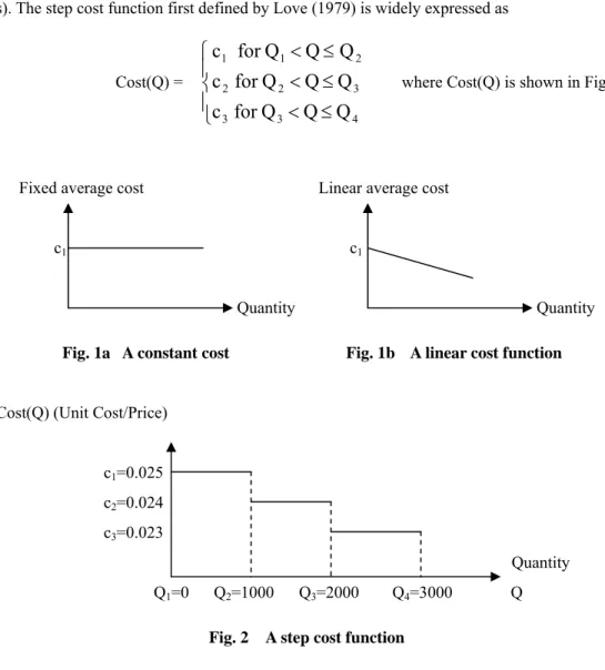
3.1 Step cost functions
One of the most commonly used discount cost functions is a step cost function as shown in Fig. 2,
in which Q1, Q2, and Q3 are the incentive quantity levels and c1, c2, and c3 are the discount costs (or
prices). The step cost function first defined by Love (1979) is widely expressed as
Cost(Q) =
⎪
⎩
⎪
⎨
⎧
≤
<
≤
<
≤
<
4 3 3 3 2 2 2 1 1Q
Q
Q
for
c
Q
Q
Q
for
c
Q
Q
Q
for
c
where Cost(Q) is shown in Fig. 2.
Fixed average cost Linear average cost c1 c1
Quantity Quantity
Fig. 1a A constant cost Fig. 1b A linear cost function
Cost(Q) (Unit Cost/Price)
c1=0.025
c2=0.024
c3=0.023
Quantity
Q1=0 Q2=1000 Q3=2000 Q4=3000 Q
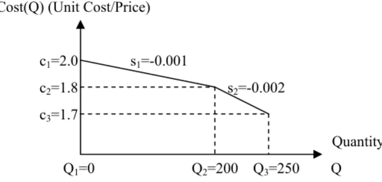
3.2 Single change point cost functions
A quantity discount schedule with a single price breakpoint is widely applied to calculate average procurement, production, inventory and transportation costs, etc. Figure 3a reveals that the starting average cost is 1.8 and declines when the required quantity increases, which implies that the slope before the quantity reaches 150 is different from that after the quantity surpasses 150. Figure 3a display a convex cost function, while figure 3b shows a concave cost function.
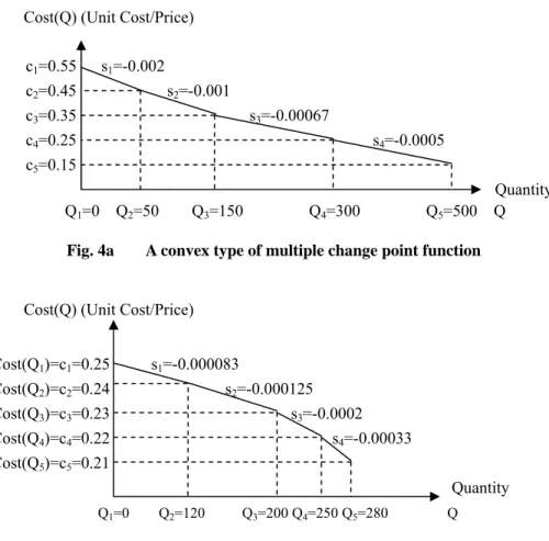
3.3 Multiple change point cost functions
Another much broadly employed cost function is a discount quantity schedule with a multiple change-point function. The function is similar to the one with a single change point function except in the number of change points, as depicted in Figs. 4a, b, and c.
Cost(Q) (Unit Cost/Price)
Cost(Q1)=c1=1.8 s1=-0.000667
Cost(Q2)=c2=1.7 s2=-0.0004
Cost(Q3)=c3=1.6
Quantity Q1=0 Q2=150 Q3 = 400 Q
Fig. 3a A convex single change-point cost function
Cost(Q) (Unit Cost/Price) c1=2.0 s1=-0.001
c2=1.8 s2=-0.002
c3=1.7
Quantity Q1=0 Q2=200 Q3=250 Q
Cost(Q) (Unit Cost/Price) c1=0.55 s1=-0.002 c2=0.45 s2=-0.001 c3=0.35 s3=-0.00067 c4=0.25 s4=-0.0005 c5=0.15 Quantity Q1=0 Q2=50 Q3=150 Q4=300 Q5=500 Q
Fig. 4a A convex type of multiple change point function
Cost(Q) (Unit Cost/Price)
Cost(Q1)=c1=0.25 s1=-0.000083 Cost(Q2)=c2=0.24 s2=-0.000125 Cost(Q3)=c3=0.23 s3=-0.0002 Cost(Q4)=c4=0.22 s4=-0.00033 Cost(Q5)=c5=0.21 Quantity Q1=0 Q2=120 Q3=200 Q4=250 Q5=280 Q
Fig. 4b A concave type of multiple change point function
Cost(Q) (Unit Cost/Price)
Cost(Q1)=c1=0.26 s1=-0.00025 Cost(Q2)=c2=0.25 s2=-0.000167 Cost(Q3)=c3=0.24 s3=-0.0001 Cost(Q4)=c4=0.23 s4=-0.0002 Cost(Q5)=c5=0.22 s5=-0.00033 Cost(Q6)=c6=0.21 Quantity Q1=0 Q2=40 Q3=100 Q4=200 Q5=250 Q6=280 Q
4. Proposed Theorems and Methods
To treat a step cost, as depicted in Fig. 2, the following theorem is introduced.
Theorem 1 A program expressed as
{Minimize Q(c1u1+c2u2+c3u3) subject to Qk+M(uk-1)≤Q≤Qk+1+M(1-uk) for k=1,2,3, u1+u2+u3=1,
where u1, u2, u3 are 0-1 variables used to indicate which cost level will be adopted based on the
required quantity} (1)
can be linearized as
{Minimize c1z1+c2z2+c3z3
subject to Qk+M(uk-1)≤Q≤Qk+1+M(1-uk) for k=1,2,3,
zk≥Q+M(uk-1), zk ≥ 0, for k=1,2,3,
u1+u2+u3=1, u1, u2, u3 ∈ {0,1},
where M is a big constant and can be set as
M = Max{Q1,Q2,Q3,Q4} } (2)
Proof To treat the product terms u1Q, u2Q, and u3Q in Program (1), the program (2) first uses z1, z2,
and z3 to replace them respectively. Consider the following Lemma.
Lemma 1
PP1: Minimize ukQ subject to uk is an 0-1 variable, Q ≥ 0.
is equivalent to
PP2: Minimize zk = ukQ
subject to zk≥Q+M(uk-1), zk ≥ 0, (3)
where M is a big value and can be set as the upper bound of Q, Q ≥ 0,
and uk ∈ {0-1}.
Lemma 1 can be verified as follows:
(i) if at optimal solution uk = 1, then equations of (3) result in zk = Q;
(ii) if at optimal solution uk = 0, then equations of (3) result in zk = 0.
Based on the Lemma 1, the program (2) can then be examined as follows:
At the optimal solution, u1+u2+u3=1 will force u1=1, u2= u3= 0, which results in Q1 ≤ Q ≤ Q2.
(ii) In case of the cost level c2 is selected
At the optimal solution, u1+u2+u3=1 will force u2=1, u1= u3= 0, which results in Q2 ≤ Q ≤ Q3.
(iii) In case of the cost level c3 is selected
At the optimal solution, u1+u2+u3=1 will force u3=1, u1= u2= 0, which results in Q3 ≤ Q ≤ Q4.
The theorem is then verified.
Take Fig. 2 as an instance, the model of optimizing this step cost function is formulated as
Minimize 0.025z1+0.024z2+0.023z3
subject to Qk+M(uk-1)≤Q≤Qk+1+M(1-uk) for k =1, 2, 3,
zk≥Q+M(uk-1), zk ≥ 0 for k =1, 2, 3, u1+u2+u3=1, u1, u2, u3 ∈ {0,1},
where Q1=0, Q2=1000, Q3=2000, Q4=3000, and M = Max{Q1,Q2,Q3,Q4} = 3000.
After inserting the constraint Q ≥ 1500 for the illustrative purpose and then executing this
program in the LINGO or Excel, the obtained solution is (u2=1, u1= u3= z1 = z3 =0, z2 = Q = 1500, the
objective value is 36, and the average cost Cost(Q) is 0.024). Building on Theorem 1 and the above demonstration, Method 1 capable of representing a general step cost function is presented below:
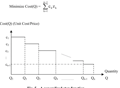
Method 1 A SCM model of optimizing a step cost function Cost(Q), depicted in Fig. 5, can be
formulated as follows: Minimize Cost(Q) =
∑
− = 1 n 1 k k kz
c
Cost(Q) (Unit Cost/Price) c1 c2 c3 : cn-1 Quantity Q1 Q2 Q3 Q4 ……… Qn-1 Qn Q
subject to
∑
− = 1 n 1 k ku
=1, uk ∈ {0,1},Qk+M(uk-1)≤Q≤Qk+1+M(1-uk) for k =1, 2, .., n-1,
zk≥Q+M(uk-1), zk ≥ 0 for k =1, 2, .., n-1,
where M is a big constant and set as M = Max{Q1,Q2, ….,Qn}, and zk stands for ukQ.
To treating single point change functions of Figs. 3a and b, the following lemmas of 2 - 4 are
introduced. In following Lemmas 2-4, Q is ordered quantity and Q1 and Q2 are the incentive quantity
levels.
Lemma 2 Based on Proposition 1 in the literature (Li and Yu, 1999, 2000), any separable linear
functions Cost(Q), shown in Figs. 3a and 3b where sk (k = 1, 2) are the slopes of line segments
between Qk and Qk+1, can be represented by
Cost(Q) = Cost(Q1)+ s1(Q-Q1)+((s2-s1)÷2))(|Q-Q2|+Q-Q2) (4)
where Q≥ 0, Q2 ≥ Q1.
Take Figs. 3a and b as illustration, by using Equation (4) we have
Cost(Q) = 1.8-0.000667Q+ (0.000267÷2) (|Q-150|+Q-150) (in Fig. 3a) (5) Cost(Q) = 2.0 – 0.001Q+(-0.001÷2) (|Q-200|+Q-200) (in Fig. 3b) (6)
where 0.000267 and -0.001 were calculated by the formula of (s2-s1) as shown in Equation (4). When
s2> s1, the break point is convex point as depicted in Fig. 3(a). Conversely, if s2< s1, the break point is
concave point as depicted in Fig. 3(b).
To linearize absolute terms with the positive coefficient in Equation (5), Lemma 3 is introduced.
Lemma 3
PP3: Minimize C = (s÷2) (|Q-g|+Q-g) subject to Q, g, s ≥ 0, is equivalent to
PP4: Minimize C’ = s(Q-g+d) subject to Q - g + d
≥
0, Q, g, d, s ≥ 0.This lemma can be confirmed as follows:
(i) if Q–g
≥
0 then at the optimal solution d = 0, which results in C’ = s(Q-g) = C;(ii) if Q – g < 0 then at the optimal solution d = g – Q, which results in C’ = 0 = C.
Take Fig. 3a as a demonstration. The model of optimizing Equation (5) is programmed as: Minimize Cost(Q)=1.8-0.000667Q+0.000267(Q-150+d)=-0.0004Q+0.000267d+1.75995 subject to Q – 150 + d ≥ 0, Q, d ≥ 0.
To linearize absolute terms with the negative coefficient in Equation (6), Lemma 4 is introduced.
Lemma 4
PP5: Minimize C=(s÷2)(|Q-g|+Q-g) subject to Q, g ≥ 0, s < 0, is equivalent to
PP6: Minimize C’ = s(Q-w+gu-g) subject to Q+
Q
(u-1)≤ w, Q, w ≥ 0, s < 0, u ∈ {0,1}, andQ
isthe upper bound of Q (Take Fig. 4b as instance,
Q
= 250).Lemma 4 can be examined as follows:
(i) if Q – g
≥
0 then at the optimal solution u=0 and w=0, which results in C’=s(Q-g)= C;(ii) if Q – g <0 then at the optimal solution u=1 and w=Q, which results in C’=0 =C. Based on Lemma 4, the model of optimizing Equation (6) can be programmed as
Minimize Cost(Q) = 2–0.001Q–0.001(Q-w+200u-200) =-0.002Q+0.001w-0.2u+2.2 subject to Q + 250 (u-1) ≤ w, Q, w ≥ 0, u ∈ {0,1}, and Q ≤ 250.
Building on Lemmas 2 - 4, Remark 1 and Methods 2 and 3 are presented as the following:
Remark 1 A single change cost function Cost(Q) where s2 > s1 as displayed in Fig. 3a is a convex
function, while Cost(Q) as displayed in Fig. 3b is a concave function where s2 < s1.
Method 2 A SCM model of optimizing a convex type of single change cost function, depicted in Fig.
3a, can be formulated as follows: Minimize Cost(Q)
subject to Cost(Q) = Cost(Q1)+ s1(Q-Q1)+(s2-s1)(Q-Q2+d2), Q-Q1+d
≥
0, and Q ≥ 0,where s2 > s1, Q1 ≥ Q2.
Method 3 A SCM model of optimizing a concave type of single change cost function, depicted in Fig.
3b, can be formulated as follows: Minimize Cost(Q)
subject to Cost(Q) = Cost(Q1)+ s1(Q-Q1)+(s2-s1)(Q-w+uQ2-Q2),
w≥Q+
Q
(u-1), Q, w ≥0, u∈
{0-1}, 0≤ Q≤Q
,where s2 < s1, and
Q
is the upper bound of Q.To treating multiple change point functions, Remark 2, Method 4, and Theorem 2 are presented as follows.
depicted in Figs. 4a, 4b, or 4c where ck= Cost(Qk), Qk are change points, and sk are slopes of line
segments between Qk and Qk+1, can be expressed as
Cost(Q) = Cost(Q1)+ s1(Q-Q1)+
∑
− = −−
1 n 2 k 1 k k2
s
s
(|Q-Qk|+Q-Qk) (7)where Q ≥ 0, 0 < Q1 < Q2< ... < Qn, and sk+1 > sk for k =1, 2, …, n-1.
To treat Equation (7) with all positive coefficients, Method 4 is introduced.
Method 4 Based on Proposition 4 in Li and Yu (2000), a SCM model of optimizing Equation (7) with
all positive coefficients can be programmed as follows: Minimize Cost(Q)
Subject to Cost(Q) = Cost(Q1)+ s1(Q-Q1)+
∑
− =
−
1 n 2 k k((s
sk-1)(Q-Qk+∑
− = 1 k 1 j jd
)) Q + d1 + d2 + ... + dn-1 ≥ Qn-1, Qk+1 - Qk≥dk, and dk ≥ 0 for k =1, 2, …, n-1.where Q ≥ 0, 0 < Q1 < Q2< ... < Qn, and sk+1 > sk for all k.
Consider the following illustration.
Example 1
Minimize Cost(Q) subject to Q ≤ 500, where Cost(Q) is depicted in Fig. 4a.
By employing Method 4, Example 1 is linearized as follows:
Minimize Cost(Q)=0.55-0.002Q+0.001(Q-50+d1)+0.00033(Q-150+d1+d2)+
0.00017(Q-300+d1+d2+d3) = -0.0005Q +0.0015d1+0.0005d2+0.00017d3+0.39999
subject to Q+d1+d2+d3 ≥ 300, 0≤d1≤150, 0≤d2≤100, 0≤d3≤50, Q ≥ 0 and Q ≤ 500.
After executing this program in the LINGO, the obtained solution is (d1 = d2 = d3 = 0, Q = 500,
and the average cost Cost(Q) = 0.15). As noted, one merit of Method 4 is that it contains only one inequality constraint and all the other constraints are bounded constraints, which could speed the computational efficiency. Although Li and Yu’s methods (1999, 2000) is quite promising to linearize a convex function, their methods either has to use k 0-1 variables to linearize a concave function with k line segment (Li and Yu, 1999) or cannot directly treat a concave function (Li and Yu, 2000). As a result, to treat Equation (7) with all negative coefficients, Theorem 2 is introduced to lessen the computational burden on treating the concave cost function.
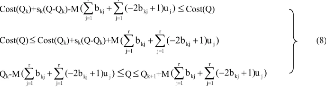
Theorem 2 A cost(Q) shown in Fig. 6 can be expressed as Cost(Qk)+sk(Q-Qk)-M( b ( 2b 1)u ) r 1 j j r 1 j kj kj
∑
∑
= = + − +≤
Cost(Q) Cost(Q)≤
Cost(Qk)+sk(Q-Qk)+M( b ( 2b 1)u ) r 1 j j r 1 j kj kj∑
∑
= = + − + (8) Qk-M( b ( 2b 1)u ) r 1 j j r 1 j kj kj∑
∑
= = + − +≤
Q≤
Qk+1+M( b ( 2b 1)u ) r 1 j j r 1 j kj kj∑
∑
= = + − +where Qk are change points, k=1, 2, …, m-1, sk are slopes of line segments between Qk and Qk+1, r is
the smallest value for 2r ≧ m-1, b
kj (j=1, 2, …,r) are assigned parameters which are derived by
1 k b 2 r 1 j kj 1 j = −
∑
=− , uj are zero-one variables, and M is a large constant.
Proof
If uj = bpj for j = 1, 2, …, r and 1
≤
p≤
m-1 (which means the p’th cost level will be adopted based onthe required quantity Q), then
∑
= r 1 j pj b + j r 1 j pj 1)u 2b (
∑
= + − = 0 and∑
∑
= = > + − + r 1 j j r 1 j kj kj ( 2b 1)u 0 b for all kexcept for k=p (i.e., k =1, 2, …, p-1, p+1, …, m-1). Consequently, all equations in (8) can be replaced as follows:
Cost(Qp)+sp(Q-Qp)
≤
Cost(Q) (9)Cost(Q)
≤
Cost(Qp)+sp(Q-Qp) (10)Cost(Q) (Unit Cost/Price) Cost(Q1) s1 Cost(Q2) s2 Cost(Q3) : : : Cost(Qk) sk Cost(Qk+1) Quantity Q1 Q2 Q3 ……… Qk Qk+1 Q
Qp
≤
Q≤
Qp+1 (11)Cost(Qk)+sk(Q-Qk)-M
≤
Cost(Q) for all k except for k = p (12)Cost(Q)
≤
Cost(Qk)+sk(Q-Qk)+M for all k except for k = p (13)Qk
≤
Q≤
Qk+1 for all k except for k = p (14)where M is a large constant.
Since only the p’th cost level is adopted based on the required quantity Q, constraints (12)-(14)
are inactive. Hence, (9)-(11) force Cost(Q)= Cost(Qp)+sp(Q-Qp) and Qp
≤
Q≤
Qp+1. In doing so,Theorem 2 is then proved.
Consider the following illustration.
Example 2
Minimize Cost(Q) subject to Q ≤ 260, where Cost(Q) is depicted in Fig. 4b.
Figure 4b displays that the break points of Cost(Q) are 0, 120, 200, 250, and 280. Hence,
referring to Theorem 2,
r
=
2
is the smallest value for 2r≥
m-1 = 4, and each bkj is derived by 1 k b 2 r 1 j kj 1 j = −
∑
= − as listed in Table 1.By employing Theorem 2, Example 2 is linearized as follows: Minimize Cost(Q)
subject to Q ≤ 260,
0.25-0.000083Q-M(u1+u2)
≤
Cost(Q)≤
0.25-0.000083Q+M(u1+u2),0.24-0.000125(Q-120)-M(1-u1+u2)
≤
Cost(Q)≤
0.24-0.000125(Q-120)+M(1-u1+u2),0.23-0.0002(Q-200)-M(1+u1-u2)
≤
Cost(Q)≤
0.23-0.0002(Q-200)+M(1+u1-u2),0.22-0.00033(Q-250)-M(2-u1-u2)
≤
Cost(Q)≤
0.22-0.00033(Q-250)+M(2-u1-u2),Table 1 The derived values of
b
kjthe k’th line segment j = 1 j = 2
1
k
=
0 02
k
=
1 03
k
=
0 14
k
=
1 1-M(u1+u2)
≤
Q≤
120+M(u1+u2),120-M(1-u1+u2)
≤
Q≤
200+M(1-u1+u2),200- M(1+u1-u2)
≤
Q≤
250+ M(1+u1-u2),250-M(2-u1-u2)
≤
Q≤
280+M(2-u1-u2),where u1 and u2 are 0-1 variables, and M is a big number.
After running this program in LINGO, the obtained solution is (u1 = u2 = 1, Q = 260, and the
average cost Cost(Q) = 0.2167). The comparison between Li and Yu’s linearization techniques and the proposed method is summarized in Table 2, which displays that to linearize a multiple change point concave function the proposed method needs much less number of 0-1 variables than Li and Yu’s method (1999) does.
As discussed in Introduction Section, the heuristic approach is also widely used to treat SCM problems with nonlinear cost functions (Shapiro, 2005). Actually, the heuristic algorithm and the mathematical model (i.e., the proposed method) have specific pros and cons, and serve different purposes. In reality, the heuristic is to generate a feasible solution to a problem at every iteration step, retain the best feasible solution between iteration steps, and the solution hold at the termination of the algorithm is deemed as the best solution. Therefore, the heuristic algorithm is appropriate to solve NP-complete (or called NP-hard) problem because its purpose is to find a best feasible solution when finishing the pre-set iteration procedures. In contrast, the proposed method is a mathematical model used to find a global optimal solution for a deterministic problem. Nevertheless, the heuristic algorithm is unsuitable to optimize a SCM problem with variable cost functions shown in Figs. 2-4, while the presented methods can linearize various types of cost functions as demonstrated in the above. Moreover, building on Method 4 and Theorem 2, a SCM model with a convex-concave type cost function as depicted in Fig 4c can also be transformed into a linear mixed integer programming program that is solvable to obtain a global optimal solution by many commercialized LP packages and SCM systems.
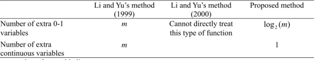
Table 2 Comparison between Li and Yu’s methods and the proposed method
Li and Yu’s method
(1999) Li and Yu’s method (2000) Proposed method
Number of extra 0-1 variables
m Cannot directly treat
this type of function log2(m )
Number of extra
continuous variables m 1
5. Solution Algorithm and Numerical Example
Notably, when unit costs are not constants, the Cost(Q) × Q (such as RM_P_Costtbsi ×
RM_P_QTYtbsi,, RM_ T_Costtbsi × RM_T_QTYtbsi, etc.) in the objective function of Model 1 will be a
product term. Accordingly, Remark 3 is introduced as follows:
Remark 3 After the necessary variables transformation (Charnes and Cooper, 1962), the objective
function with product terms in the proposed SCM quantitative model can be straightly solved by a linear programming.
Consider the following illustration.
Example 3
Minimize Cost(Q) × Q (15)
subject to Cost(Q) = -0.002Q+0.001w-0.2u+2.2,
Q + 250 (u-1) ≤ w, 0≤ Q ≤ 250, w ≥ 0, u is a zero-one variable, where Cost(Q) is depicted in Fig. 3b.
The objective function of Cost(Q) × Q involves three product terms of Q×Q, Q×w, and Q×u. Based on Remark 2 and using the variable transformation, Q×Q, Q×w, and Q×u can be replaced by Q’, w’, and u’, respectively. In doing so, Q×Q + 250 (u-1) ×Q ≤ w×Q and 0≤ Q×Q ≤ 250Q are incurred. As a result, Program (15) can be reformulated as follows:
Minimize Cost(Q)’ (16)
subject to Cost(Q)’ = -0.002Q’ +0.001w’ - 0.2u’+ 2.2Q ,
Q+250(u-1)≤w, 0≤ Q ≤ 250, w ≥ 0, u is a zero-one variable,
Q’+250u’-250Q ≤ w’, 0 ≤ Q’ ≤ 250Q,
where Cost(Q)’, Q’, w’, and u’ denote Cost(Q) × Q, Q×Q, Q×w, and Q×u, respectively.
Noteworthy, since u is a zero-one variable in Programs (15) and (16), the product term Q×u cannot be simply represented by u’ without other constraints. Accordingly, based on Lemma 1, Program (16) is then re-programmed as follows:
Minimize Cost(Q)’ (17)
subject to Cost(Q)’ = -0.002Q’ +0.001w’ - 0.2u’+ 2.2Q,
Q+250(u-1)≤w, 0≤ Q ≤ 250, w ≥ 0, u is a zero-one variable,
where M can be specified as 250 (the upper bound of Q).
The constraint Q ≥ 165 is added into Example 3 for the illustration. After executing the program (17) in LINGO or Excel, the computed solution is (u = w = 0, Q = 165, the average cost of Cost(Q) = 1.87, and the total cost of Cost(Q)×Q = 280.5) which is the optimal solution as obtained in Program (15). Consider another demonstration.
Example 4
Minimize Cost(Q) × Q (18)
subject to Cost(Q) =-0.0005Q +0.0015d1 +0.0005d2+0.00017d3+0.39999,
Q+d1+d2+d3 ≥ 300, 0≤d1≤150, 0≤d2≤100, 0≤d3≤50, 0≤ Q ≤ 500,
where Cost(Q) is depicted in Fig. 4a.
Suppose the average cost of Cost(Q) is a multiple change cost function as depicted in Fig. 4a.
By using the variable transformation, Q×Q, Q×d1, Q×d2, and Q×d3 can be replaced by Q’, d’1, d’2, and
d’3, respectively. In doing so, Q’+d’1+d’2+d’3 ≥ 300Q, 0 ≤ d’1≤150Q, 0 ≤ d’2 ≤100Q, 0 ≤ d’3 ≤ 50Q, and
0≤ Q’≤ 500Q are incurred. Due to no 0-1 variable existing in Model (16), therefore, Example 4 can be straightly reformulated as
Minimize Cost(Q)’ (19)
subject to Cost(Q)’= -0.0005Q’ +0.0015d’1 +0.0005d’2+0.00017d’3+0.39999Q,
Q+d1+d2+d3 ≥ 300, 0≤d1≤150, 0≤d2≤100, 0≤d3≤50, 0≤ Q ≤ 500,
Q’+d’1+d’2+d’3 ≥ 300Q, 0≤d’1≤150×Q, 0≤d’2≤100×Q, 0≤d’3≤50×Q, 0≤ Q’ ≤ 500Q.
For the illustrative purpose, the constraint Q ≥ 265 is added into Example 4. After executing the
program (19) in LINGO, the computed solution is (d1 = d2 = 0, d3 = 35, Q = 265, the average cost
Cost(Q) = 0.27344, the total cost Cost(Q) × Q = 39.747345) which is the optimal solution as found in Program (18).
Based on the above illustration, a solution algorithm is described as follows to solving a general SCM problem.
Solution Algorithm
Step 1. Use Model 1 to formulate a generalized SCM problem.
Step 2. Use Methods 1 - 4 and Theorem 2 to treat various types of cost functions such as nonlinear step functions, nonlinear concave functions, and nonlinear S-curve functions.
Step 3. Transform product terms into single variables. Since the rule of variables transformation is simple and distinct, a computer program is easily coded to handle variables transformation.
Step 4. Solve the problem by available commercialized packages such as LINGO or EXCEL.
Step 5. Execute sensitive analysis and coordination and negotiation among supply chain partners. Thereafter, the most feasible and promising supply chain plan is scheduled.
Example 5
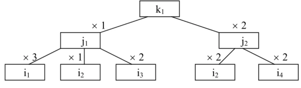
In the consumer electronics industry, semi-products j1 and j2 are composed of (three units i1, one
unit i2, and two units i3) and (two units i2 and two units i4), respectively. The finished product k1
consists of one j1 and two j2 units. The bill of material (BOM) and the entire supply chain of the
product k1 are displayed in Figs. 6 and 7, separately. According to customer orders from (c1, c2, c3, c4),
they require the k1 goods (300, 355, 320, 340), (360, 370, 350, 280) and (350, 375, 275, 360) at times
t2, t3, and t4, respectively.
According to procurement contracts in this example, the purchasing costs between BSs and ISs and between ISs and factories involve transportation costs. To simplify this illustration, assume all
raw materials i1, i2, i3, and i4 hold the same unit purchasing and transportation cost. Unit purchasing &
k
1× 1 × 2
j
1j
2× 3 × 1 × 2 × 2 × 2
i
1i
2i
3i
2i
4Fig. 7 The bill of material (BOM) of the product k1
C
1F
1W
1B
1S
1C
2F
2W
2B
2S
2C
3F
3W
3Beginning Intermediate C
4Suppliers Suppliers Factories Warehouses End
Customers
transportation costs for (b1 to s1, b2 to s1, b1 to s2, b2 to s2) are (0.023, 0.02, 0.02, Cost(Q)), (0.024,
0.021, 0.021, Cost(Q)), (0.025, 0.022, 0.022, Cost(Q)), and (0.024, 0.021, 0.021, Cost(Q)) for all raw
materials at the t1, t2, t3 and t4 time separately, where the Cost(Q) is depicted in Fig. 2. Assume all
semi products have the same purchasing and transportation cost. Unit procurement and transportation costs for (s1 to f1, s1 to f2, s1 to f3, s2 to f1, s2 to f2, s2 to f3) at the t1, t2, t3 and t4 time are (0.2, 0.5, 0.1, 0.3,
0.2, 0.4), (0.15, 0.45, 0.15, 0.35, 0.25, 0.45), (0.1, 0.45, 0.2, 0.25, 0.2, 0.35), and (0.15, 0.4, 0.1, 0.3, 0.15, 0.3), respectively.
To simplify the calculation, over the time, unit transportation costs from f1 to w1, f1 to w2, f1 to w3,
f2 to w1, f2 to w2, f2 to w3, f3 to w1, f3 to w2, and f3 to w3 are 0.6, 0.4, 0.3, 0.3, 0.5, 0.4, 0.55, 0.4, and 0.4,
separately. Unit transportation costs from each w1, w2, and w3 to each c1, c2, c3, and c4 are 0.04, 0.03,
0.03, 0.04, 0.02, 0.03, 0.04, 0.03, 0.04, 0.03, 0.02, and 0.03 separately, for all time. Average production
costs for k1 in (f1, f2, f3) are (1.75, 1.8, G_M_Cost), (1.77, 1.79, G_M_Cost), (1.76, 1.78, G_M_Cost),
and (1.75, 1.8, G_M_Cost) at t1, t2, t3 and t4 time, respectively, where G_M_Cost is specified in Fig. 3a.
Average outsourcing costs of k1 for f1, f2, and f3 are all same as specified in Fig. 3b over the entire
period. Unit production costs for (j1, j2) in s1 and s2 are (1.7, 1.75) and (1.75, 1.65) for all time.
Inventory capacities of (raw materials, semi-products), (semi-products, finished goods) and (finished goods) for all suppliers, factories, and warehouses separately are (50, 50), (150, 150) and (30) for all period. The maximal capacity of each factory to produce k is no more than 250 and
manufacturing capacities in s1 and s2 are not restricted in this example. The total outsourcing amount of
k1 cannot exceed 600 units for each factory. Unit inventory costs for (i1, i2, i3, i4, j1, j2) in s1 and s2 are
separately (RM_I_Cost, 0.3, 0.2, 0.3, 0.4, 0.45) and (RM_I_Cost, 0.3, 0.3, 0.2, 0.43, 0.4) for all time,
where RM_I_Cost is specified in Fig. 4c. Unit inventory costs for (j1, j2, k1) in f1, f2 and f3 separately
are (0.2, PSFG_I_Cost, 0.6) (0.3, PSFG_I_Cost, 0.55) and (0.3, PSFG_I_Cost, 0.5) for all time where
PSFG_I_Cost is displayed in Fig. 4a. Unit inventory costs for k1 in w1, w2, and w3 are respectively 0.3,
0.35, and 0.35 over the time.
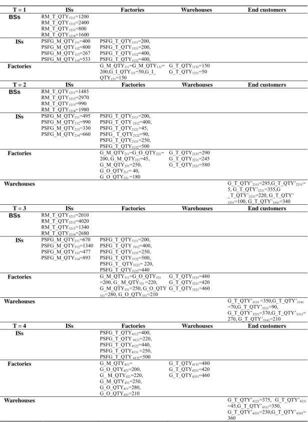
After finished Steps 1 – 4 in Solution Algorithm, the computed supply chain schedule by running LINGO is summarized in Table 3. By employing the presented techniques, logistical managers along intersecting supply channels can negotiate and mutually cooperate to optimize supply chain schedule throughout the entire supply chain (since the solution generated by the global optimal solution can conveniently perform sensitivity analysis). In Step 5, by exploiting the computer’s powerful capability of computing and exchanging information, the management can adjust and coordinate the entire supply chain schedule until partners within the supply chain have committed the schedule.
Table 3 The generated solution for Example 5
T = 1 ISs Factories Warehouses End customers
BSs RM_T_QTY1211=1200 RM_T_QTY1212=2400 RM_T_QTY1213=800 RM_T_QTY1214=1600 ISs PSFG_M_QTY111=400 PSFG_M_QTY112=800 PSFG_M_QTY113=267 PSFG_M_QTY114=533 PSFG_T_QTY1111=200, PSFG_T_QTY1131=200, PSFG_T_QTY1112=400, PSFG_T_QTY1132=400,
Factories G_M_QTY111=G_M_QTY131=
200,G_I_QTY111=50,G_I_
QTY131=150
G_T_QTY1131=150
G_T_QTY1311=50
T = 2 ISs Factories Warehouses End customers
BSs RM_T_QTY1211=1485 RM_T_QTY1212=2970 RM_T_QTY1213=990 RM_T_QTY1214=1980 ISs PSFG_M_QTY211=495 PSFG_M_QTY212=990 PSFG_M_QTY213=330 PSFG_M_QTY214=660 PSFG_T_QTY2111=200, PSFG_T_QTY 2112=400, PSFG_T_QTY2121=45, PSFG_ T_QTY2122=90, PSFG_T_QTY2131=250, PSFG_T_QTY2132=500
Factories G_M_QTY211=G_O_QTY221=
200, G_M_QTY221=45, G_M_QTY231=250, G_O_QTY211= 40, G_O_QTY231=180 G_T_QTY2131=290 G_T_QTY2211=245 G_T_QTY2321=580
Warehouses G_T_QTY’2111=295,G_T_QTY’2211=
5, G_T_QTY’2221=355,G
_T_QTY’2231=220, G_T_QTY’ 2331=100, G_T_QTY’2341=340
T = 3 ISs Factories Warehouses End customers
BSs RM_T_QTY3211=2010 RM_T_QTY3212=4020 RM_T_QTY3213=1340 RM_T_QTY3214=2680 ISs PSFG_M_QTY311=670 PSFG_M_QTY312=1340 PSFG_M_QTY313=477 PSFG_M_QTY314=893 PSFG_T_QTY3111=200, PSFG_T_QTY 3112=400, PSFG_T_QTY3131=250, PSFG_T_QTY3132=500, PSFG_T_ QTY3121= 220, PSFG_T_QTY3122=440
Factories G_M_QTY311=G_O_QTY321
=200, G_ M_QTY321 =220, G_M_QTY331=250, G_O_QTY 311=280, G_O_QTY331=210 G_T_QTY3131=480 G_T_QTY3211=420 G_T_QTY3321=460
Warehouses G_T_QTY’3131 =350,G_T_QTY’3141
=70,G_T_QTY’3211=90,
G_T_QTY’3221=370,G_T_QTY’3311=
270, G_T_QTY’3341=210
T = 4 ISs Factories Warehouses End customers
ISs PSFG_T_QTY4112=400, PSFG_T_QTY 4121=220, PSFG_T_QTY4122=440, PSFG_T_QTY4131 =250, PSFG_T_QTY 4132=500 Factories G_M_QTY411= G_O_QTY421=200, G_ M_QTY421=220, G_M_QTY431=250, G_O_QTY411=280, G_O_QTY431=210 G_T_QTY4131=480 G_T_QTY4211=420 G_T_QTY4331=460
Warehouses G_T_QTY’4121=375, G_T_QTY’4131
=45,G_T_QTY’4311=350,
G_T_QTY’4331=230,G_T_QTY’4341=
6. Concluding Remarks
Although the importance of computer based quantitative models for coordinating supply chain activities is undoubted, their successful power depends heavily on the effectiveness and availability of mathematical formulation. Therefore, the establishment of a mathematical model to interpreting practical supply chain behavior and thus helping enterprises perform complex, laborious, and even trivial analysis has been a challenging and difficult task for a long time (Holmstrom and Hameri, 1999). Although Lemmas 2-4 presented by Li and Yu (1999, 2000) can be efficiently employed to tackle a convex cost function, their methods have some deficiencies in treating a concave function. Consequently, compared to current SCM quantitative models, the proposed methods have the following features:
(1) The proposed techniques can straightforward treat widespread logistic cost functions. For example, Method 1 is presented to treat a step function with Theorem 1 and Lemma 1, Methods 2 and 3 are presented to treat a single change point cost function with Lemmas 2-4, and Method 4 is proposed to treat a concave type of multiple change point function.
(2) Logistical managers can easily arrange and adjusting an entire SCM schedule via negotiation and cooperation with supply chain partners, since the yielded solution is optimal and sensitivity analysis can be performed conveniently.
(3) The presented model can be easily coded in current computer program to aid the management in handling SCM, because of the simple and distinct methods developed herein.
(4) The formulated SCM model can also be executed using many available commercialized packages, such as LINGO and Excel.
(5) The proposed model offers available-to-promise and handles the fulfillment of orders with the total cost minimization, due to synchronization of the capacitated supply, production, outsourcing, inventory, and distribution along intersecting supply chains.
References
Anderson, D. R., Sweeney, D. J., and Williams, T. A., Quantitative Methods for Business, 9th ed.,
Cincinnati, Ohio: International Thomson, 2004.
Charnes, A. and Cooper. W. W., “Programming with Linear Fractional Functions”, Naval Research Logistics, Vol. 9, No. 1, 1962, pp. 181-186.
Science, Vol. 6, 1960, pp. 465-490.
Cohen, M. A., Fisher, M., and Jaikumar, R., “International Manufacturing and Distribution Networks: A Normative Model Framework. In Ferdows, K. (Eds.), Managing International Manufacturing, Holland: Elsevier Science, 1989, pp. 67-93.
Council of Supply Chain Management Professionals (CSCMP), Supply Chain Management/Logistics Management Definitions, http://www.cscmp.org/Website/ AboutCSCMP/Definitions/Definitions.asp, (2006).
Drucker, P. F., “Physical Distribution: The Frontier of Modern Management. In Bowersox, D. J., LaLonde, B. J., and Smykay, E. W. (Eds.), Readings in Physical Distribution Management: The
Logistics of Marketing, London: Macmillan, 1969, pp. 3-8.
Forrester, J. W., Industrial Dynamics: A Major Breakthrough for Decision Makers, Harvard Business
Review, Vol. 36, No. 4, 1958, pp. 37-66.
Handfield, R. B. and Nichols Jr., E. L., Introduction to Supply Chain Management, New Jersey: Prentice Hall, 2005.
Hanssmann, F., “Optimal Inventory Location and Control in Production and Distribution Networks”,
Operations Research, Vol. 7, 1959, pp. 483-498.
Holmström, J., Korhonen, H., Laiho, A., and Hartiala, H., “Managing Product Introductions across the Supply Chain: Findings from a Development Project”, Supply Chain Management, Vol. 11, No. 2, 2006, pp. 121-130.
Holmstrom, J. and Hameri, A. P., “The Dynamics of Consumer Responses: A Quest for the Attractors of Supply Chain Demand,” International Journal of Operations & Production Management, Vol. 19, No. 6, 1999, pp. 993-1009.
Ishii, K., Takahashi, K. and Muramatsu, R., “Integrated Production, Inventory and Distribution Systems, International Journal of Production Research, Vol. 26, No. 3, 1988, pp. 473-482.
Li, H. L. and Yu, C. S., “A Global Optimization Method for Nonconvex Separable Programming Problems”, European Journal of Operational Research, Vol. 117, No. 1, 1999, pp. 275-292.
Li, H. L. and Yu, C. S., “Solving Multiple Objective Quasiconvex Goal Programming Problems by Linear Programming”, International Transactions in Operational Research, Vol. 109, No. 1, 2000, pp. 59-82.
Love, S., Inventory Control, New York: McGraw-Hill, 1979.
Oum, T. H. and Waters, W. G. II, “A Survey of Recent Developments in Transportation Cost Function Research”, Logistics and Transportation Review, Vol. 32, No. 4, 1996, pp. 423-463.
Ross, D. F., Competing Through Supply Chain Management, Chicago: Chapman & Hall, 2005.
Shapiro, J. F., Modeling the Supply Chain, 2nd ed., Singapore: Duxbury, 2005.
Shaw, A. W., Some Problems in Market Distribution, Cambridge: Harvard University Press, 1915, pp. 7-12.
Slats, P. A., Bhola, B., Evers, J. J. M., and Dijkhuizen, G.., “Logistic Chain Modeling”, European
Journal of Operational Research, Vol. 87, No. 1, 1995, pp. 1-20.
Sodhi, M. S., “Managing Demand Risk in Tactical Supply Chain Planning for a Global Consumer Electronics Company”, Production and Operations Management, Vol. 14, No. 1, 2005, pp. 69-79. Stevens, G. C., “Integrating the Supply Chain”, International Journal of Physical Distribution and
Materials Management, Vol. 19, No. 1, 1989, pp. 3-8.
Tan, E. N., Smith, G. and Saad, M., “Managing the Global Supply Chain: A SME Perspective”,
Production Planning & Control, Vol. 17, No. 3, 2006, pp. 238-248.
Tayur, S., Ganeshan, R., and Magazine, M., Quantitative Models for Supply Chain Management, Boston: Kluwer, 2006.
Vidal, C. J. and Goetschalckx, M., “A Global Supply Chain Model with Transfer Pricing and Transportation Cost Allocation”, European Journal of Operational Research, Vol. 129, No. 1, 2001, pp. 134-158.
Yu, C. S., “Single-Item Multi-Period Robust Supply Chain Model for Coordinating Logistical Supply and Sales Efforts”, Taiwan Academy of Management Journal, Vol. 6, No. 1, 2006, pp. 1-36.