Regression analysis based on semicompeting risks data

Regression Analysis Based on Semicompeting Risks Data

Author(s): Jin-Jian Hsieh, Weijing Wang and A. Adam Ding

Source: Journal of the Royal Statistical Society. Series B (Statistical Methodology), Vol. 70, No.

1 (2008), pp. 3-20

Published by:

Wiley

for the

Royal Statistical Society

Stable URL:

http://www.jstor.org/stable/20203808

.

Accessed: 30/04/2014 19:51

Your use of the JSTOR archive indicates your acceptance of the Terms & Conditions of Use, available at

.

http://www.jstor.org/page/info/about/policies/terms.jsp

.

JSTOR is a not-for-profit service that helps scholars, researchers, and students discover, use, and build upon a wide range of

content in a trusted digital archive. We use information technology and tools to increase productivity and facilitate new forms

of scholarship. For more information about JSTOR, please contact [email protected].

.

Wiley and Royal Statistical Society are collaborating with JSTOR to digitize, preserve and extend access to

Journal of the Royal Statistical Society. Series B (Statistical Methodology).

J. R. Statist Soc. B (2008)

70, Part 1, pp. 3-20

Regression

analysis

based on semicompeting

risks

data

Jin-Jian Hsieh and Weijing Wang

National Chiao-Tung University, Hsin-Chu, Taiwan and A. Adam Ding

Northeastern _{University, Boston, USA} [Received July 2005. Final revision July 2007]

Summary. Semicompeting risks data are commonly seen in biom?dical applications in which

a terminal event censors a non-terminal event. Possible _{dependent censoring complicates} sta tistical _analysis. We consider _{regression analysis} based on a non-terminal event, say disease

progression, which is subject to censoring by death. The methodology proposed is developed for

discrete covariates under _{two types of assumption. First, separate copula} models are assumed

for each covariate group and then a flexible regression model is imposed on the progression time which is of major interest. Model checking procedures are also proposed to help to choose

a best-fitted model. Under _{a two-sample setting,} Lin and co-workers _{proposed a competing}

method which requires an additional marginal assumption on the terminal event and implicitly

assumes _{that the dependence} structures _{in the two groups} are the same. _Using simulations, we

compare the two approaches on the basis of their finite sample performances and robustness properties under model misspecif?cation. The method proposed is applied to a bone marrow

transplant data set.

Keywords: Copula model; Dependent censoring; Model selection; Multiple events data;

Transformation model

1. Introduction

Many medical studies involve analysis of multiple end points. Such events may be classified into two types, namely terminal and non-terminal. Death _{is an example of terminal events in the} sense that its occurrence precludes the development of others. Examples of non-terminal events, which are subject to censoring by a terminal event, include disease progression or recurrence. If

the relationship between the two events is completely unspecified, the marginal distribution of the time to a non-terminal _{event is not identifiable owing to possible dependent censoring.}

Let X be the time to the non-terminal _{event of major interest, which is usually a status of} disease progression, and let Y be the time to death and C be the time to the external cen

soring event. Observed variables consist o?? = IaFaC, Y = YaC, 6x = I(X^7aC) and 6y = I(Y < C). Such a data structure was called semicompeting risks data by Fine et al. (2001). There has been increasing research attention in developing statistical methods _{for analysing}

semicompeting risks data. For example, investigation of the degree of association between the two events has been pursued by Day et al (1997) and Fine et al (2001) in which the Clayton model is assumed _{and Wang (2003) for a class of copula models.}

Address for correspondence: Weijing Wang, Institute of Statistics, National _{Chiao-Tung University, Hsin-Chu,} Taiwan.

E-mail: [email protected]

4 _{J.-J. Hsieh, W. Wang and A. A. Ding}

In this paper, we consider regression analysis based on progression time X. Because of depen dent censoring, the marginal distribution of X _{is not identifiable non-parametrically.} Under a

two-sample setting, Lin et al. (1996) and Chang (2000) modelled the marginal effects on both X and Y but did not specify their joint distribution. Specifically Lin et al. (1996) considered a

bivariate location-shift model _{and Chang (2000) assumed a bivariate accelerated} failure time model. This research direction has been further extended _{to general regression settings in which}

the non-terminal _{event is generalized to be recurrent events (Ghosh and Lin, 2003; Lin and} Ying, 2003) whereas death still serves as a terminal event. The technique of artificial censoring

is used in these references to handle _{the problem of dependent censoring. Despite being theo} retically appealing, the efficiency of the resulting estimator is affected by the degree of artificial censoring. Furthermore, these methods implicitly assume that the dependence structures for the

two groups, or for all the levels of covari?tes, are the same. In other words, they do not account for the situation _{that covariates may affect the dependence} structure.

Here we adopt a different approach to assessing the covariate effect on progression time under dependent censoring. Without making any assumptions on the marginal distribution of Y, we assume that

h(X) = -Zf6 + e, (1)

where Z is the pxl discrete covariate vector, 6 is the pxl parameter vector, h(f) is a monotonie increasing function and s is the error term. The parameter 6 which measures the covariate effect on X _{is of major interest. Model (1) can be classified} into two classes. One class assumes that h(t) is a known monotone function but leaves the distribution of s to be unknown. For example, when h{t) = t, the model becomes a location-shift model; when h(t) = log(i), the model follows an accelerated failure time model. The other class assumes _{that h(t) is unknown but the distri} bution of e is completely specified. Examples of the second class include the Cox proportional hazard model _{with s being the Gumbel} extreme value distribution _{and the proportional} odds model with s being the standard logistic distribution.

To handle _{the problem of non-identifiability,} we assume _{that (X, Y) jointly follow an Archi} medean _{copula (AC) model in the upper wedge V} = _{{(x, y) : 0 < x ^ y < oo} such that}

?r(X>x,Y^y)

=

0-^a{?r(X^x)}

+ (l)a{Vr(Y>y)}l

where _{(/> : [0,1] -> [0, oo] has two continuous} derivatives _{on (0,1) and satisfies 0(1) = 0, d(f)(t)/dt < 0} and d2(?(t)/dt2 > 0 for all 0 < t < 1. Examples of AC models include the Clayton (1978) model

(?a(v) = (v~a - I) I a (a > 0), the Frank model (1979) <?>a(v) = log{(l - a)/(I - av)} (a > 0), the Gumbel _{(1960) model </>a(v)} = _{{- logii;)}0^1 (a > 0) and the log-copula model <?>a(v)} = _{1 -

log(v)/aj}a+l ? 1 (a, 7 > 0). In the presence of discrete covariates, we assume separate AC models for each covariate _{group to account for the possibility} that the dependence structures for different groups are different. To simplify the notation, let Fz (x, y) = Pr(Z ^ x, Y ^ y | Z = z), Fx,z(jc) = Pr(X ^ x\Z = z) and Fy>z(y) = Pr(F ^ y\Z = z). We assume that

FZ(X, y) = _{^}az[<t>z,az{Fx,z(X)}} + <l>Ztaz{Fy9z(y)}l (2)

Note _{that, for different groups, we allow not only a different association parameter} az but also different _{forms of 0z,az(-).}

The inference method _{proposed for estimating} 6 under models _{(1) and (2) is discussed} in Section 2. In Section 3, we propose model checking procedures to verify the copula assump

tion in model _{(2) and to select an appropriate regression model in equation} (1). Simulation results and data analysis are presented in Section 4. Section 5 contains some concluding remarks.

Regression Analysis 2. _{A two-stage} inference _procedure

Let (Xi, Yi) (i ? 1,... 9n) be independent realizations of (X9 Y) which follow model (2) in the upper wedge. The/?-dimensional covariate vector for subject / is denoted as Z?, which takes discrete values, say zi,...,zk- Denote _{n^ = E?=1/(Z?} = _{zjO as the number of observations} for the A:th subsample and n = _Y,?=lnk. Let Q (i = 1,... 9n) be independent and identically dis tributed realizations _{of the external censoring variable C which is assumed to be independent} of (X, Y). We observe semicompeting risks data {(Xi, 6Xi, Yi, 6y?, Z\) (i ? 1,2,..., n)}, where Xi = Xi A Yi A Q, Y i = Yi A Cu Sx,i = KXi < Yt A Q) and 6y? = I(Yt < Q). The inference proce

dure proposed contains two steps. The parameters in model _{(2), namely cxz, FyiZ(y), Fz(x, y) and} Fx>z(x), are estimated in the first stage. In the second stage, the proposed estimating function of

9 is constructed _{on the basis of the estimator of FXiZ(x).}

2.1. _{First-stage: estimating} nuisance _parameters

First we obtain the estimators _{of Fz(x, j), FyiZ(y), Fx,z(x), G(y)} = _{Pr(C ^ y) and cxz, which are} denoted _{as Fz(x, y), FyyZ(y), Fx,z(x), G(y) and az respectively, by applying existing methods} in

the literature to the subsample with Z = z.

For x ^ y9 it follows that Fz(x, y) = Fr(X ^x,Y^y\Z = z)/G(y). Hence, using the plug-in approach, Fz(x, y) can be estimated by

Fz(x,y) = PT(X^x,Y^y\Z = z)/G(y) = Zl(Xi>x,Yi^y,Zi = z) nzG(y), (3)

i=l '

where

G(y)= El f

1 - E I(Yi = u,6yi =

0)/ E KYi^u)}.

This estimator _{is based on the assumption} that covariates Z do not affect the distribution of censoring variable C In the situation that the distribution of C depends on discrete covariate Z, G(y) can be modified by the corresponding Kaplan-Meier estimator Gz(y) which uses only

those data points with Z/ = z. Similarly the estimator of Fy,z(y) is given by

Fy,z(y)

=

E IM > y, Zi

=

_{z)/nz G(y). (4)}

i=l '

There are several estimators _{of az based on semicompeting risks data. Assuming the Clayton} model _{in the upper wedge, the estimating function that was proposed by Day et al (1997) was}

constructed _{on the basis of 2 x 2 tables and that proposed by Fine et al (2001) utilized the con} cordant information _{for paired observations. Wang (2003) generalized the former approach to} general AC models. In the absence of covariates, her estimating function of ce can be expressed as

L(a,fj)=n

l

_{/ /}

w(x,y){Nn(dx,dy)-?n(dx9dy;a9f))}9

(5)

where w(x9 y) is a weight function,

0q,r)(x, y) N\p(dx9 y) Nqi (x9 dy) 0a,v(x9 y) N\o(dx9 y) + R(x9 y) - Nio(dx9 y)

'

Nn(dx9dy) = _JZKXi=x9Yi = y9?xi = \98yi = \)9

?=l

JVio(dx,y) = _? I(Xi=x96xi = \9Y{>y)9

J.-J. Hsieh, W. Wang and A. A. Ding

Noi (x, dy) = _? I(Xi > x, Y i = _{y, 8yi} = 1),

i=\

R(x,y) = Zl(Xi^x,Yi>y) and _{0a,n(x9 y)} = _{9a{F(x9 y)} with}

~

d2cj>a(v)/dv2

0'?

and 77 = F(x9 y) can be estimated by i) = F(x9 y) by using formula (3) without further partitioning byZ.

Here we modify Wang's method to estimate az by using only data points with Z[ ? z. Then, on the basis of model _{(2), we can derive Fx^z(x) in terms of 0z,az(O, Fz(x9 y) and Fy,z(y). Fine et al.} (2001) suggested to consider the relationship on the diagonal line y = x and, by straightforward calculation, we obtain

The marginal function FXyZ(x) can be estimated by

Kz(x)

=

_{<?zXS$z,az{Fz(x>x)}-<?z^ (6)}

2.2. Second _{stage: estimating the regression parameter}

The proposed estimating equation of 9 is motivated by the following two-sample test statistic with Z = 0,1. Specifically to test Fx$ (t) = FXi \ (t) for every t within the range of the data, we can

use

UT

=

\/(^r)

_/

W^ {^oW

-

FX9i(x)}dx,

(7)

where W(x) is a weight function.

Now we modify the test statistic Uj in equation (7) to construct an estimating equation for one-dimensional _{6 with Z = 0,1. Let #o be the true value of 9. Model (1) induces a functional} transformation _{?#( ) such that ?e0(Fx,o)} = _{FXy\. When h(-) is known but the distribution} of e is unknown, ??(F)(t) = F[h~l{h(t) + 9}]; when h(-) is unknown but the distribution of s is known, ?e(F)(t) = Fs[F~l{F(t)} + 9], where Fs(t) = Pr(e > t) denotes the survival function of e. Now we can define a function g(t9 9) such that

g(t,9) = te(Fx,o)(t)-FxA(t). Then g(t, 90) = 0 for all t. Since

A

_)!'

U(e)=y/(^)Jw(x)g(x,e)?x

= 0,

where g(t,?) = &(Fx,0)(t) - FxA(t).

The above idea can be modified to account for the situation _{that Z contains multiple} cova riates but all of them have finite discrete values. In such a case, let {zk, k ? 1,2,..., K} denote

Regression Analysis

the set of all possible Z-values. Now zk, 0 and #o are p x 1 vectors. When model (1) is true, it follows that

?(z._Zk)j0o(Fx,Zk) = Fx,Zj. Here and throughout the paper, aT denotes the trans pose of a. Define _gkj(t9 0) = tzp(FXtZk)(t) - FXtZJ(t) and gkj(t9 0) = _{?zp(FX9Zh)(f)} - Fx,Zj(t), where Zkj = zj ? Zk and FXiZk is the estimator (6) based on the subsample 4ith Z ? zk- The estimating function then becomes

U(6) = ? ^oiz^ZkjJi-^-)

[kJ Wkj(t)

gkj(t9

9) dt (8)

where wo(-) and Wkj(-) are the weight functions, and tkj is the largest value of X in the pooled subsample with Z = zk or Z = zj. The proposed estimator of 9 is the solution to U(6) = 0, which is denoted as 9.

Asymptotic properties of 9 which solves U(9) = 0 are given in the following theorem.

Theorem 1. Assume that models _{(1) and (2) hold. Under the regularity conditions} that are stated in Appendix A, 6 is a consistent estimator of #o and ?1/2(0 - 9o) is asymptotically normal with mean 0, where #o is the true value.

A sketch of the proof is outlined in Appendix B. More detailed discussions _{are provided in} Hsieh _{et al (2007). Since it is not easy to estimate the asymptotic variance of 9 by an analytic}

formula, we suggest the use of a bootstrap or a jackknife method to estimate its variance. In practice, the weight function may also be estimated. Replacing Wkj(t) in equation (8) with Wifc/(0> we have the estimating function

U(9) = ? wo(zjje)zkjj(^L-)

[kJ Wkj(t) gkj(t9

9) dt.

+ nj/ Jo

The Gehan-type weights are often used (page 230 of Klein and Moeschberger (2003)); these can be written as

y

, _(nk+nj) GZk(x) GZj(x)

nicGZk(x)+njGZj(x)

where GZk(x) is the Kaplan-Meier estimator _{of GZk(x)} = Pr(C ^x\Z = zj?)- Note that _Wkj(x) is an estimator of ^ _ (ck + Cj) GZk (x) GZj (x) Wkj (x) ? ? / N ? -~r~ > ckGZk(x) + CjGZj(x)

where _{ck and Cj are the constants} that are defined in the first regularity condition (a) that is listed in Appendix A. Let 9 solve ?(9) = 0. Its asymptotic properties are stated in the following theorem. _{In Appendix} C, we present a sketch of the proof and, for the details, refer to Hsieh et al (2007).

Theorem 2. If _{Wkj(t) uniformly strongly converges} to _{Wkj(t) then, under the conditions} for theorem _{1, the solution to the estimating equation ?(9)} = 0 is also _{asymptotically} normal, i.e. let 9 denote the solution _{to ?(9) = 0; then nl/2(9} ? _{9o) weakly} converges to a mean 0 normal random variable, where 9o is the true value.

For computation, we may use the fact that F^o (0 and FXi \ (t) are piecewise constant functions. Let i(i) ^... ^ t(n) be the observed ordered times of X in the pooled sample and set i(0) = 0. Then Fx^o(t) and FXi\(t) are constants on the time intervals (?(?_i),?(?)]. Usually, the estimated weight

functions _{such as the Gehan-type weights can also be taken to be piecewise constant functions} between _{t(i-\) and fy) which would enable simplification for computation. For example, with}

8 _{J.-J. Hsieh, W. Wang and A. A. Ding}

piece wise constant weight function W(t)9 the quantity correponding to Uj in equation (7) can be rewritten as

UT=j(n^-)

? ^(/))(?(o-?(?-i)){^,o(?(o)-^,ia(/))}.

(9)

For _{illustration, we now derive the estimating equations} under _{a two-sample setting for} selected examples.

2.2.1. _{Example 1 : Cox proportional hazard model}

When s has the extreme value distribution, model (1) becomes the Cox proportional hazard model. _{Then F?(t) = exp{-exp(i)} and ?0(F)} = FexP(?). When 9 equals its true value 00, it fol

lows that

Fx,i(x) = FXt0(x)^?o\

Therefore _{g(t9 9)} = _^,o(Oexp(6,) - _{Fx^(t)9 and the estimating equation} is

0(6) =

^/(^)

_jf

??

W(t){Fx,o(trm

-

FXil(t)}

d/ = 0.

Under _{the piecewise constant weight function, the resulting estimating equation becomes}

U(9) =

_J(?)

_{? W(?(o)(?(0 -?(/_i)){Fx,o(?(/))exp(0)}

-

_?,l(?(0)}

= 0

2.2.2. _{Example 2: the proportional} odds model

When _{s is the standard logistic distribution, model (1) becomes the proportional} odds model, where F?(t) = 1/{1 +exp(0} and ?e(F) = F/{exp(<9) - F exp(0) + F}. When 9 equals its true

value #o, it follows that

Fx,i(t) = exp(?o) - Fx,o(Oexp(?o) + F,,0(f) ' and ( g. _ _{_^C,0(0_F (} v

9{ '

exp(0)

-

F,,o(Oexp(fl) + FXf0(t)

X'U h

So the estimating equation is

&(W(?)

_{V V n / Jo}

P

*? ?--^-*-/UoU=o.

\ exp(0)

-

FXt0(!)expW

+ Fxfi(t)

*''

J

Under _{the piecewise constant weight function, the resulting estimating equation becomes}

Regression Analysis 2.2.3. _{Example 3: the accelerated failure time model}

When h(t) = log(0, model (1) becomes the accelerated failure time model. Now ?o(F)(t) = F{exp(0)i}. When 9 equals its true value 0o, it follows that

Fx,i(t) = Fx,o{exp(90)t}9 and

9(t, 9) = Fx,o{exp(90)t} -

FxA(t). So the estimating equation is

U(9) =

y/(^)

_j

W(t)[Fx,o{exp(9)t}

-

Fx?(t)]dt

= 09

where F,j0{exp((9)i} = Pr{X ^ exp(0)i|Z = 0} = Pr{exp(-0)X ^ t\Z = 0}. Note that the discon tinuous points of FXjo{exp(?)i} are different from those of Fx^(t). Denote Fx0(t) as the estima tor FXio(t) computed on the basis of the transformed data

{Qxp(-9)Xi,Qxp(-9)Yi,6xi,6yi}

for / with Zi = 0. Let ?(i) ^... ^ t(n) be the order times of the pooled sample {exp(-o)X//(Z/ = 0) + X//(Z/ = l)(/=l,...,n)}.

If the weight function is piecewise constant and takes jumps at {ty), j = 1,..., n], the resulting estimating function becomes

?m=*/(?)

e w(k))(h) -k-i))iKo(h))

-

KiChq)}=0.

v v n J i=l

3. Model selection

The procedure proposed is developed on the basis of two assumptions: the dependence structure of an AC model characterized _{by (?z,az(') *n m?del (2) and the regression model in expression}

(1). By specifying the dependence relationship between X and Y for each value of Z, we can avoid making unnecessary assumptions about the covariate effect on Y as in Lin et al (1996). Now we discuss how to justify the assumptions imposed.

3.1. Selection _{of a copula model}

We first consider how to check whether _{a copula model 4>z,az(-) fits the data at hand for each} covariate group. Without loss of generality and to simplify the presentation, the discussions here are based on a homogeneous sample {(Xi, 6Xi, Yi, 6yi) (i=l,2,...,n)} such that (X, Y) follows an AC model

F(x, y) = Ca{Fx(x), Fy(y)}

=

0"1 [0Q{FX

(*)} + <t>a{Fy(y)}].

(10)

We briefly summarize our ideas. Consider the function Fn(t\, ^) = Pr(X ^ t\, Y ^ ti \6X = _{1, 6y} = 1) which is identifiable non-parametrically in the upper wedge {(t\, tj) : 0 < t\ ^ ti < oo}. By com paring the non-parametric estimator of Fn(t\, ti) and its model-based estimator for F11 (t\, tj) on the basis of some distance measure, we can find the most plausible model which is the model

that yields the smallest distance among the candidates. Furthermore a formal goodness-of-fit test can be constructed if the distribution of the distance measure _{under the null hypothesis can be} derived. Since analytic derivations are complicated, we suggest using the bootstrap resampling method to obtain the cut-off value in the test.

10 _{J. -J. Hsieh, W. Wang and A. A. Ding}

The non-parametric estimator, which is denoted as F _{(t\, ti) (t\ ^ ?2), is given by}

Zl(Xi^tuYi^t29Sxi

=

\98yi

=

_l)/?

/(&/ = 1,^

= 1).

i=l ' i=\

Assume that there are K model candidates _{C$?{Fx(x), Fy(y)} (k=l929...9K)9} each of which can be characterized _{by (ft?. Note} that the definition _{of a depends on the model chosen. For} an AC model _{that is indexed by (ft?, the model-based estimator, which is denoted} as _{Fk (t\, ti),} can be computed over the region {t\ ^ ?2} as follows:

roo _ry Jy?ti Jx=t]

F\\t^2)=JyTrXrT

Fk(dx9dy)G(y)

Fk(dx9dy)G(y)

Fk(x9 y) -Fk(x + dx9y) - Fk(x9 y + dy) + Fk(x + dx, y + dy) and Fk(x9 y) =

^?

i^t\Fx{x)} + (j)f{Fy{y)}]. To verify whether a copula model (ft? fits the data, we can per

form a formal testing procedure as follows. Consider testing Ho'.(/)a = (ft? versus H^'.^a^ (ft? Define

D*=sup|F11(?i,?2)-F?1(?i,f2)|. (H)

We _{can reject Ho if Dk > c^, where c? is the critical value satisfying Pr(D^ > ck\Ho) = 7, the} prespecified type I error rate.

Because the distribution of Dk is difficult _{to derive analytically, we suggest using bootstrap} resampling methods to obtain the cut-off value, /?-value and power. Here we briefly describe the procedure. A bootstrap sample under model (ft? can be generated as follows. Recall that, given

the original data, we have obtained G(c)9 Fy(y) and Fx(x) under the assumption of model (ft?. Then generate (Uf, V?) ~ copula model k with U? ~ i/(0,1) and _Vf ~ t/(0,1). Then set _Xf =

s if Fx(s+) < 1 - Uf < Fx(s)9 Y*=t if Fy(i+) < 1 - V* < _FyQ and C* - G(c). Given (Xf, Y*9 Cf) (i= 1,...,?), we can construct a bootstrap sample {(X? , 6*i9 Yt , <?* ) (?=1,2,_,n)}9

where X* = Xf a^*a Cf, f

*

=

Ff a Cf, ?*.

=

/(Xf < If A Cf) and ?*.

=

/(If < C*). With a

bootstrapped sample, we can compute the corresponding values of Dk. Repeating the boot strapping procedure many times, the distribution of Dk can be approximated by the empirical counterparts from the bootstrapped samples.

The above tests will reject the null hypothesis if the data obviously violate the copula model (ft?. In practice, we may be more interested in choosing the best-fitted copula model from several candidates _{that are indexed by k} = _{1,2,..., K. For this, we can select the model that yields the}

smallest Dk. Now we derive theoretical properties of the model selection procedure proposed. Theorem 3. Assume that (X9 Y) follow model (10) and both variables are continuous and the

independent censoring variable C has bigger support than the supports of X and Y. Suppose that there are K model candidates _{in the AC family. Let the kth model C$?(u, v) be charac} terized by (ft?(t)9 which has regular analytic properties in / and is continuous in a, whose parameter space is a closed set. If (ft? is the true copula model, Dk -+F 0 as n -> 00. If (ft? is not the true model, Pr?liminf^oo?//) > 0} = 1. Furthermore let k denote _{the copula model}

that yields the smallest Dk among all the candidates. Then (ft? is consistent if the true copula model is included in the list of candidates.

In Appendix D, a sketch of the proof for theorem 3 is given. A more detailed proof can be found in section 3 of Hsieh _{et al. (2007).}

Regression Analysis 3.2. Selection of the covariate model

After _specifying the form of model _{(2), our procedure requires choosing an appropriate regres} sion model _{in expression (1). If model (1) is correctly specified, gy (t, 9o)} = 0 and it is reasonable to expect that faj it, 9) is closer to zero for the correct model than a wrong model for moderate sam ple sizes. This fact can be used to check the model assumption (1). Let Dr = max?,;,? \gkjif, 9)\. A formal model _{checking procedure can be formulated as testing the hypothesis Ho', the form of} model _{(1) is correct versus H^: the form of model (1) is not correct. The null hypothesis is rejected}

if Dr is too big. The cut-off value for the test can be calculated by applying the bootstrapped method which can also be used for model selection. _Suppose that there are several choices for model _{(1), say model k ? 1,2,..., K. To select the best-fitting model, we can simply choose the} model with smallest _DhR, where _DkR is calculated under model k.

4. Numerical _analysis 4.1. Simulation results

We designed several simulation settings to examine the validity and robustness of the methods proposed. Data generation algorithms for the Clayton model and the Frank model have been given in Prentice and Cai (1992) and Genest (1987) respectively. In the following analysis, we

set the weight functions as _wo(z-;#) = 1 and

(ni + n j) GZj (x) Gz. (x)

Wij(x)

= \

J

Zl

\

J

.

niGZi(x)+njGZj(x)

For each estimator under evaluation, the average bias and the standard deviation based on 1000 runs are reported. Here we describe only summary information of the numerical settings. For the details, refer to section 4 of Hsieh et al (2007).

Tables 1 and 2 contain _{the results of the first analysis that compared our proposed estima} tor 9 and 9^, the estimator of Lin et al (1996). We set (e,Q\Z to follow an AC model with Z = 0,1. Then, on the basis of (s, ?, Z), the value of (X, Y) can be determined from the models

hx(X) = -90Z + s and h2(Y) = -770Z + ?. Here we set 90 = r?o = 0.5 and n0 = n\ = 150. Note that all the assumptions are satisfied for 9. However, in the evaluation of 0l, the covariate model for X _{is correct but the assumption} about common _{dependence structures for the two groups} or the extra assumption on a covariate model for Y may be misspecified.

In the four cases in Table 1, we consider the location-shift model with h \ (t) = hi (t) = t. We shall

Table 1. Finite _{sample performance} of two estimators evaluated under _{four situations!}

Model _<9L 6

Case 1 _{-0.0026 (0.0934) -0.0025 (0.0909)} Case 2 _{-0.0013 (0.1136) 0.0969 (0.0849)} Case 3 _{0.0022 (0.0950) -0.0122 (0.0888)} Case 4 _{0.0008 (0.1100) 0.0982 (0.0840)}

fThe correlation structures are the same for two covari ate groups in the first case and different in the last three cases. The first number is the average bias of the estimator and the number _{in parentheses} is the standard deviation based _{on 1000 replications.}

12 _{J. -J. Hsieh, W. Wang and A. A. Ding}

Table 2. Finite _{sample performance} of two estima tors evaluated under four situations with different covariate models _{for progression} time and death time

(thus 6\_ becomes invalid)!

Model _0L 0

Case 5 -0.0041 _{(0.0974) 0.0890 (0.1175)} Case 6 -0.0067(0.1135) 0.3387(0.1127) Case 7 _{0.0025 (0.1156) 0.0884 (0.1170)} Case8 _{0.0125(0.1152) 0.3793(0.1081)}

f The first number is the average bias of the estimator and the number _{in parentheses} is the standard devia tion based on _{1000 replications.}

use the notation _{{Clayton(ro), Frank(ri)}} to denote the situation _{that one group with Z = 0 fol} lows the Clayton model with r = to and the other with Z = 1 follows the Frank model with r = r\. The dependence structures for the four cases are case _{1, {Clayton(0.5),Clayton(0.5)},} case 2, {Clayton(0.8),Clayton(0.1)}, case 3, {Frank (0.5), Clay ton (0.5)}, and case 4, {Frank(0.8), Clayton(O.l)}. In case 1 where the conditions for both estimators are valid, #l slightly outper

forms 9. However, in the last three cases, #l is biased. It seems that the bias of 0l is affected more _{by the discrepancy} in the level of associations _{for the two groups than the difference} in

the dependence structures.

Table 2 contains the results for another four conditions _{(cases 5-8). We set h\(t) = t but} h2(t) = log(i), which is a condition that violates the assumption that was made by Lin et al

(1996). The dependence structures in these four cases follow the same pattern as in cases 1-4 in Table 1. _{We see that 9 outperforms #l even more since, for the latter, the two types of assumption}

are both misspecified.

The second analysis checks the validity of the proposed method for selecting an appropriate copula model. Suppose that there are two copula models under consideration, where model k = 1 is the Clayton model and model k ? 2 is the Frank model. First we set the Clayton model as the true model and n = 150. The mean and standard deviation _{(in parentheses)} of Dl and D2 are 0.0780 _{(0.0187) and 0.1397 (0.0304) on the basis of 1000 replications.} The percentages of

successfully selecting the Clayton model are 93.4% on the basis of the order of Dj 0 = 1,2). Then we set the Frank model as the true model. The mean and standard deviation _{(in parentheses)}

ofD1 _{and D2 are 0.1398 (0.0330) and 0.0819 (0.0206). The percentages} of successfully selecting the Frank model are 92.3% on the basis of the order of Dj (7 = 1,2). Finally, we examine the proposed testing procedure by using the resampling method. Under the Clayton model, we set up the goodness-of-fit test Ho : the data follow the Clayton model versus H&: the data do not fol

low the Clayton model. By resampling 1000 times, we obtained Dx = 0.0511 with/>-value 0.909 and the cut-off value c\ =0.1004 (at 0.05 significance level). Hence hypothesis Ho is accepted, which is the correct decision. _{For the same data set, we ran the analysis again with Ho : the data}

follow the Frank model versus Ha: the data do not follow the Frank model. We obtained that D2 = 0.1247 with/?-value 0.012; the cut-off value (7 = 0.05) c2 = 0.1058. Accordingly we reject hypothesis Ho, which is also the correct decision.

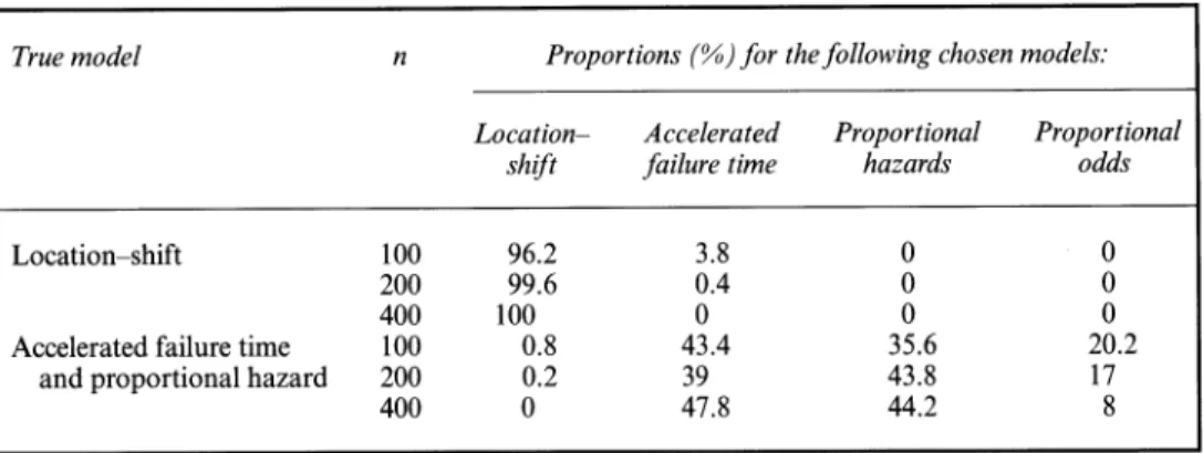
Under the Clayton model with to = 0.5 and r\ = 0.6, we examine the method proposed that was introduced in Section _{3.2 for selecting an appropriate regression model.} Table 3 lists the proportions of each model being selected by the method proposed on the basis of 500 simulation

Regression Analysis Table 3. _{Proportion of the covariate models that were selected by the method proposed} on the basis of 500 replications!

True model _Proportions (%) for the following chosen models:

Location- Accelerated _{Proportional Proportional} shift failure time hazards odds

Location-shift

Accelerated failure time and proportional hazard

100 200 400 100 200 400 96.2 99.6 100 0.8 0.2 0 3.8 0.4 0 43.4 39 47.8 0 0 0 35.6 43.8 44.2 0 0 0 20.2 17

|The first column lists the true covariate model; the second column _{lists the sample} size; the last four columns contain _{the proportion} of each of the four covariate models selected.

Table 4. _{Finite sample performance of 01}

Model Results _{for the following} models:

Location-shift Accelerated failure time Proportional hazard Proportional odds

Clayton Frank -0.0024(0.1113) -0.0015(0.1105) -0.0042(0.1016) 0.0011(0.0995) 0.0029(0.1736) 0.0058(0.1662) -0.0084(0.1734) -0.0094(0.1661) -0.0022(0.1507) -0.0032(0.1514) 0.0067(0.1544) -0.0096(0.1680) 0.0039 (0.2683) -0.0023 (0.2633) -0.0028 (0.2573) 0.0013(0.2602)

f The first number in each column is the average bias of 9\, the second number in parentheses is the standard deviation _{of 9\ based on 1000 replications,} the third number _{is the average bias of ?2 and the} fourth number in parentheses is the standard deviation _{of ?2 based on 1000 replications.}

larger. When the true model changes to the accelerated failure time and proportional hazard models, which are both correct in our setting, these two models together are chosen most of

the time. As n increases, the proportion of a correct decision _{also increases (79% when n} = _100, 82.8% when n = 200 and 92% when n = 400).

We also examined _{the situation of multiple covariates. With Z'} = _{(Z(1), Z(2)) in which Z^ (j} = 1,2) are both binary, the sample can be portioned into four groups with Z\ = (0,0) (r = 0.2), Z'2 = (0,1) (r = 0.3), Z'3 = (1,0) (r = 0.4) and Z\ = {\91) (r = 0.5). The sample size in each of

the four groups is 75. We evaluated two dependence structures, namely Clayton and Frank, and four regression models, namely location-shift, accelerated failure time, proportional hazard and proportional odds, for each of which _9f0 = (0.3,0.3). The average bias and the standard deviation on the basis of 1000 simulation _{runs are reported in Table 4. The results show that}

the method _{proposed still performs well under various regression settings.}

4.2. _{Data analysis}

The methodology proposed is applied to the bone marrow transplants data that were given in Klein _{and Moeschberger (2003), page 484. There were 137 leukaemia patients receiving bone} marrow _{transplants. Let X be the time to relapse of leukaemia,} Y be the time to death and C

14 _{J. -J. Hsieh, W. Wang and A. A. Ding}

be the time from transplant to the end of study. Let SX = I(X ^ Y a C) be the relapse indica tor and let _6y = _{I(Y < C) be the death indicator. The sample can be divided into three groups} with Z' = (0,0) indicating the acute myelogenous leukaemia _{(AML) low risk group, Z' = (0,1)} indicating the acute lymphoblastic leukaemia (ALL) group and Z' = (1,0) indicating the AML high risk group. The regression model of interest is h(X) = -Z'9 + s, where 9' = (9\, 92) which measures whether the disease _{type affects the relapse time.}

For each covariate group, we test the hypothesis Ho'.^a^ Clayton model versus Ha: not Ho. By bootstrapping 1000 times, the/?-values of Dc for the AML high risk group, the ALL group and the AML _{low risk group are 0.752,0.656 and 0.177 respectively. Hence the Clayton model} is adopted for all three groups. Using Day's method (or equivalently Wang's method) to estimate rz, we obtain f(o,o) =0.7485 (0.1176), f(0,i) = 0.7894 (0.0853) and fa,o) =0.7685 (0.0872), where the number _{in parentheses} is the estimated standard derivation _{by using the jackknife method.} The above analysis implies that the dependence structures _{in the three groups are similar and}

the two events are highly correlated.

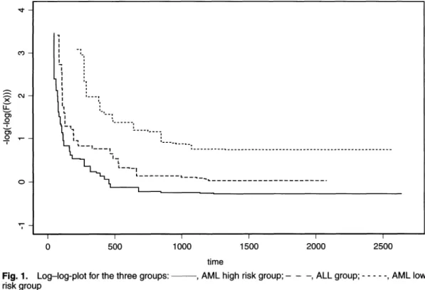
Then we choose a model _{for measuring the group effect on X. Fig. 1 shows the fitted log-log} plot of Fx(x) for the three groups. Since the three curves look parallel, we choose the proportional hazard model to measure _{the group effect. On the basis of the method} that was described in Section 3.2, we can formally test the proportional hazard model _{assumption. By bootstrapping}

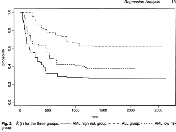
1000 times, we obtain/?-value 0.774 which _{implies that this model is appropriate. Fig. 2 depicts} the three survival curves of Fx(x). Under the proportional hazard _{regression model} and the Clayton assumption for each covariate group, we obtain 9\ = 1.3624 (0.3765) and 92 = 0.9503

(0.3984). The results show that the risk of relapse for the AML high risk group is 3.9 times that of the risk for the AML _{low risk group, and the risk for the ALL group is 2.59 times that of the} AML _{low risk group. The difference is statistically significant.}

o D)

O i

500 1000

Fig. 1. Log-log-plot for the three groups:

risk group

1500

time

,

AML high risk group;

2000 2500

-

Regression Analysis JQ C? -Q O 00 ? CO O ? CM O q i-1-r 0 500 1000 1500 2000 2500 time

Fig. 2. Fx(t) for the three groups:-, AML high risk group;-, ALL group;., AML low risk group

5. _Concluding remarks

In this paper, we model the failure time to a non-terminal _{event by a flexible transformation} model. To handle the problem of dependent censoring, we make an additional assumption that,

for each covariate group, failure times for the two types of event follow a copula model in the identifiable _{region. Model checking procedures are also proposed to examine the appropriate} ness of these two model _{assumptions. Compared with existing methods such as that proposed by} Lin et al. (1996), our approach allows for different dependence structures _{in each group, avoids} making additional modelling assumptions on the terminal event and utilizes all the data with

out paying the price for artificial censoring. The simulation analysis confirms our conjecture that the estimator _{that was proposed by Lin et al. (1996) becomes unreliable if the dependence} structures _{in the two groups are different.}

The strategy proposed for checking the copula assumption is to compare the non-parametric estimator with its model-based estimator of a chosen reference function, say Fn(t\9t2). This

technique is similar to that used in Wang and Wells (2000). For possible future research, one may examine how to choose such a function or a combination of several functions that contain most of the model information that is characterized _{by </>( ) so that the corresponding test pro} cedure would detect the departure from the null hypothesis better and hence give higher power. To select an appropriate regression model for the non-terminal event, a formal model checking

procedure is also proposed by using the bootstrap method. The regression method proposed can handle multiple covariates with discrete values. Extension to continuous covariates must face the challenge of imposing additional regression assumptions on model (2) or adopting some non-parametric techniques like smoothing. This goes beyond the scope of the current paper but may deserve further investigation. Note that in model (3) we suggest use of the Kaplan-Meier

16 _{J. -J. Hsieh, W. Wang and A. A. Ding}

estimator _{based on data {(Y/, 1} - _{6yi) (i} = _{1,...,n)} to estimate G(t). Since C is also censored} by X a F, another estimator based on data {(X?, 1 - 6x?6x?) (i = 1,...,n)} can be constructed. Obviously the latter yields a worse estimator of G(t). However, it has been shown in other con

texts, such as in Tsai and Crowley (1998), that plugging in a worse estimator of the nuisance parameter sometimes improves the result.

Acknowledgements

The first two authors were funded by the National Science Council of Taiwan. Part of the work was done while the second author was visiting the Institute for Mathematical Sciences, National University of Singapore, in 2005. The visit was supported by the Institute.

Appendix A: Regularity conditions of theorem 1 Let

?(e) =

_{J2^o(z?jO)zkjj(^1-)}

_[

"

Wkj(t) gkj(t90)

dt (12)

where ck = \imn^ (nk/n)9 and (0, Tkj) is the support of X in the subgroup with Z = zk or Z = Zj. To derive

large sample properties of 9, we assume the following regularity conditions. (a) As n

-

oo, ck = \imn^ (nk/n) > 0 for all k values.

(b) For each Z = zk, the HZk(u, v, a) has bounded partial derivatives with respect to u9 v and a, where

Hz(u, v9 a) = _{4>^a{4>z,a(?)} + 4>z,a(v)} is defined in model (2).

(c) For each Z = zk, the standard regularity conditions hold for estimating Fz (x,x) and FyiZk(x) (e.g. conditions for theorem 6.3.2 in Fleming and Harrington (1991)) so that nk/2{FZk{x9x) ? FZk{x9x)}

and

nkl/2{FyfZk(x) ?

Fy,Zk{x)} converge weakly to Gaussian processes.

(d) The weight functions wo(x) and Wkj(t) are positive and bounded and w0(x) is differentiate with

continuous derivatives.

(e) For each of the two classes of model (1), we impose the following assumptions:

(i) for the first case, h(t) is differentiate, h'(t) ^0 and is continuous, Wkj(t) = Wkj{t)/h'(t) is differ entiate and _{f | Wkj(t) | at < oo;}

(ii) for the second case, the distribution of s has a density f?(t) which is differentiate with bounded

derivatives._

(f) The function U(6) which is defined in equation (12) is differentiable with respect to 9 and the

matrix

is non-singular. Furthermore ?(9) ^0for9^90 _{and liminf^H-??,|?(0)| >0.}

Appendix B: Sketch of proof for theorem 1

Here we provide a brief sketch of the proof of theorem 1; the details are given in Hsieh et al (2007). Consider

U(9) = ? w0(zTkj0)zkj

_j{

_{nkln)^ln

\

_{fk} Wkj(t)}

gkJ(t,

9) at,

k<j J v {nk/n + nj/n) J0

where Wkj(t) is a deterministic function. Equation (A.5) in Hsieh et al (2007) states that U{9)/nl/2 converges (in probability) to

?(9) = ? woiz^zkjjf^1-)

[

^

Wkj(t) gkj(t,

9) at,

Regression Analysis

in which the convergence is uniform in 0. Consider a compact set Dr = {|| 0 - 00 || ^ r} where r is a positive constant. By assumption (f) U(0) ^ 0 for 0 =? 0O and liminf||0|Koo|?/(0)| > 0; then the continuity of U(0) implies that infp-o0\l>r\U(6)\ >0. The (uniform) convergence of U(0)/nl/2 to U(0) implies that there will be no solution for U(0) = 0 outside the compact set Dr when n is large. Since this is true for every r > 0, 0

is consistent.

By Taylor series expansion we obtain

U(0) = 0 = U(00)

_{+ ? ?-1/(0)(0,}

-

0/fO), (13)

?

(0\,...,0P)T. Hence we have the expression

?(?^

'?t/(e))",/2('-?0)=-i/(?0)-

(14)

The statement of expression (A.6) in Hsieh et al. (2007) is about the convergence of

n['? du i

to

locally uniformly at 0 = 60. Using this condition along with the consistency of 0, we can show that

^(?^-

?^"(?^

^

which, by assumption (f), is a non-singular constant matrix. By expression (A.7) in Hsieh et al. (2007), U(Oo) is asymptotic normal with mean 0. Therefore nl/2(0 ? 0O) is asymptotic normal with mean 0 because

it has the same asymptotic distribution as

-i -^?(6,),...,^-?(6,))

U(6o).

This _{completes the proof.}

Appendix C: Sketch of proof for theorem 2

Compared with the previous proof, we need to show only that

(a) {?(0) ? U(0)}/n?/2 uniformly strongly converges to 0,

(b) 3[{i/(0) - U(0)}/ni/2]d0i strongly converges to 0, which takes place locally uniformly at 0 = 00, and (c) ?(6o) ? U(Oo) strongly converges to zero.

Firstly, ?(0)-U(0)

₌

E wo(zTkjO)zkj

_j{

(nk/n^nj/"

\ f kJ{Wkj(t)

-

Wkj(t)} gkj(t,

0) dt.

(15)

Under the related regularity conditions and the uniform and strong convergence of Wkj(t) to Wkj(t), we can establish the uniform and strong convergence of expression (15) to 0. So condition (a) holds.

Secondly, we can write

?(00)

-

U(0o)

=

_{E woizJjO?Zkj}

_j{

_{(nk/nlnj/" } ftkJ{Wkj(t)}

-

Wkj(t)} n1'2

gkj(t,

00) dt.

(16)

k<j J v [rik/n + nj/n) Jo

Under the related regularity conditions as well as nl/2 gkj(t, 00) = Op(\) for all t and Wkj(t) - Wkj(t) = ?^(1),

18 _{J. -J. Hsieh, W. Wang and A. A. Ding} Finally

_d_ j u(0) -

u(0)

'dot A/2 --Ewo(zle)ZkjZkj,i k<j

+

_EH;0(?/)^7

./n)nj/n \

?

n + nj/nf Jo

(17)

The required regularity conditions plus the uniform strong convergence of Wkj(t) to Wkj(t) imply that the first term in equation (17) converges uniformly (in 6) and strongly to 0. To prove the second term, we need

to consider _{the two regression} classes _separately.

For the first case that &(F)(0 = F[h~l{h(t) + 0}],

k<j

_{"*4W{;?^}?[f<*?*,-*"w,fc*}

*,*

=

??.<i/>a,7{iT!Ti7Ll

k<j

J

v {nk/n + nj/n)

*

?

(See the proof of expression (A.4) in Hsieh et al. (2007).) Note that local boundedness of l/h'[h~l {h(t*) - zJjO}] can be established owing to the continuity of h'(t). The related regularity conditions and the result of expression (A.4) in Hsieh et al (2007) imply that the second term in equation (17) locally uniformly

strongly converges to 0.

For the second case that ?e(F)(t) = Fe[F~l{F(t)} + 0], then ?'0(F)(t) = fe[F-l{F(t)} + 0]. Hence

E woizlQztj

_j{

_{nktn)^ln

₎

A

_[

r{Wkj(t)

-

Wkj(t)}

gkj(t,

0) dt

k<j J V {nk/n+rij/n) dOiUo

=

Z^(zTkj0)zkjj\

(nk/nln^

\

[tkJ{Wkj(t)-Wkj(t)}zkjj

fe[F^{F(t)} + zTkj0]dt,

Wkj(t) to Wkj(t) and the boundedness of fe[F~x { F (t)} ~\- _zjj?], i.e. the second term in equation (17) locally

uniformly strongly converges to 0.

In summary equation (17) locally uniformly strongly converges to 0, i.e. condition (b) holds. This com pletes the proof.

Appendix D: Sketch of proof for theorem 3

First, the empirical distribution function is uniformly consistent, i.e. supfl^,2 \F (t\, t2) ? Fn(t\,t2)\^ Q

as n ? co. Then it can be shown _{that, for t\ ^ t2, Fk (t\, t2) uniformly converges} to

p?? py

/

/

_{Fk(dx,dy,?)G(y)}

where FkCdx, dy, ?) = Fk(x y, ?) - Fk(x + dx, y, ?) - _{Fk(x, y + dy, ?) + Fk(x + dx, y + dy,_?) and Fk(x, y} ?) = _{(j)f [<t>f{Fx(x)} + (t)f{Fy(y)}].} If 0^ is the true copula model, then a^pa _{and F?x(tx,t2,a) uni}

formly converges to Fn(t\,t2). Therefore, Dk -^p 0.