IEEE TRANSACTIONS ON NEURAL NETWORKS, VOL. 7, NO. 3, MAY 1996 709
Reinforcement Learning for An ART-B ased
Fuzzy
Adaptive Learning Control Network
Cheng-Jian Lin and Chin-Teng Lin, Member, IEEEAbstract- This paper proposes a reinforcement fuzzy adap- tive learning control network (RFALCON) for solving various reinforcement learning problems. The proposed RFALCON is constructed by integrating two fuzzy adaptive learning con- trol networks (FALCON’S), each of which is a connectionist model with a feedforward multilayer network developed for the realization of a fuzzy controller. One FALCON performs as a critic network (fuzzy predictor), and the other as an ac- tion network (fuzzy controller). Using the temporal difference prediction method, the critic network can predict the external reinforcement signal and provide a more informative internal reinforcement signal to the action network. The action net- work performs a stochastic exploratory algorithm to adapt itself according to the internal reinforcement signal. An ART-based re- inforcement structurdparameter-learning algorithm is developed for constructing the RFALCON dynamically. During the learning process, both structure learning and parameter learning are performed simultaneously in the two FALCON’S. The proposed RFALCON can construct a fuzzy control system dynamically and automatically through a rewardlpenalty signal (i.e., a “good“ or “bad” signal). It is best applied to the learning environment, where obtaining exact training data is expensive. The proposed RFALCON has two important features, First, it reduces the combinatorial demands placed by the standard methods for adaptive linearization of a system. Second, the RFALCON is a highly autonomous system. Initially, there are no hidden nodes (i.e., no membership functions or fuzzy rules). They are created and begin to grow as learning proceeds. The RFALCON can also dynamically partition the input-output spaces, tune activation (membership) functions, and find proper network connection types (fuzzy rules). Computer simulations have been conducted to illustrate the performance and applicability of the proposed learning scheme.
I. INTRODUCTION
OST of the supervised and unsupervised learning algo-
M
rithms for neural networks require precise training data for setting the link weights and link connectivity of the nodes for various applications. For some real-world applications, precise training data are usually difficult and expensive, if not impossible, to obtain. For this reason, there has been a growing interest in reinforcement learning algorithms for neural networks [1]. In this paper, we are extending our previous work on fuzzy adaptive learning control networks (FALCON’S) [2] to the reinforcement learning problem.Training data are very rough and coarse for the reinforce- ment learning problem, and they are only “evaluative” when Manuscript received May 26, 1994; revised January 29, 1995 and May 26, 1995. This work was supported by the National Science Council, Republic of China, under Grant NSC 83-0422-E-009-004.
The authors are with the Department of Control Engineering, National Chiao-Tung University, Hsinchu, Taiwan, R.O.C.
Publisher Item Identifier S 1045-9227(96)01228-3.
compared with the “instructive” feedback in the supervised learning problem. Training a network with this kind of eval- uative feedback is called reinforcement learning; this simple evaluative feedback is scalar and is called the reinforcement signal. In addition to the roughness and noninstructive nature of the reinforcement signal, a more challenging problem to reinforcement learning is that a reinforcement signal may only be available at a time long after a sequence of actions has occurred; this signal may be caused by an action several time steps before or by the whole sequence of actions with varying degrees of contribution. In the latter case, it is difficult to determine which action to reward or punish. For example, in chess, the final result (win or lose) cannot be known until after a long sequence of moves. This is the well-known credit assignment problem in artificial intelligence [3]. To solve the long time-delay problem, reinforcement learning systems need the capability to predict. Reinforcement learning that is able to predict is also much more useful than supervised learning schemes in dynamic control problems, since the success or failure signal might be known only after a long sequence of control actions. From the biological and cognitive points of view, reinforcement learning is much closer to the modern animal learning theory [4] than is supervised learning. Research shows that animals and most cells adapt themselves to environments according to reinforcement signals from the external world or other cells. Moreover, animals can learn extensively about their environments even before the external reinforcement signal as introduced in [ 5 ] . This situation is very similar to learning many high-level intelligent actions such as how to drive a car.
The development of reinforcement learning can be roughly divided into two stages. The first began in the 1950’s when mathematical psychologists developed computational models to explain the learning behavior of animals and human beings [ 6 ] . They viewed learning as stochastic processes and devel- oped the so-called stochastic learning model. At almost the same time, cybemeticians and control theorists were making independent efforts in the study of stochastic learning. Their work basically used deterministic automata as a model for learning systems operating in stationary random environments, and later the model was generalized to use stochastic automata [7]. At this stage, most of the learning models were “nonas- sociative” since there was no input to the learning system except the reinforcement signal. A typical example is the two- armed bandit problem [8]. More details on stochastic learning automata can be found in [9]. Representative of the second stage development of reinforcement learning is the associative
i
710 IEEE TRANSACTIONS ON NEURAL NETWORKS, VOL. 7 , NO. 3, MAY 1996 reinforcement learning in which people try to associate an
input pattern with output patterns according to a reinforcement signal. This was stimulated by the theory proposed by Klopf [ 101. Inspired by Klopf‘s work and earlier simulation results [ 111, Barto and his colleagues used neuron-like adaptive elements to solve difficult learning control problems with only reinforcement signal feedback [12]. The idea of their proposed architecture, called the actor-critic (adaptive heuristic critic) architecture, was fully developed in [13]. They also proposed the associative reward-penalty (AR-P) algorithm for adaptive elements called Aa-p elements [14], and several generalizations of AR-P algorithm have been proposed [15]. Williams formulated the reinforcement learning problem as a gradient-following procedure [17], and he identified a class of algorithms, called REINFORCE algorithms, that possess the gradient ascent property. These algorithms, however, still do not include the full AR-P algorithms. Recently, Berenji and Khedkar [ 181 proposed a fuzzy logic controller and its associ- ated learning algorithm. Their architecture extends Anderson’s method [ 191 by including a priori control knowledge of expert
operators in terms of fuzzy control rules. Lin and Lee [20] also proposed a reinforcement neural-network-based fuzzy logic control system (RNN-FLCS) for solving various reinforcement learning problems. The R”-FLCS can find proper network structure and parameters simultaneously and dynamically.
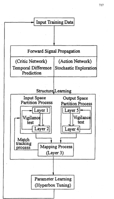
In this paper, we shall apply the technique of associative reinforcement learning to our proposed reinforcement FAL- CON system. The proposed learning system can construct a fuzzy controller automatically and dynamically by means of a reward-penalty (i.e., good-bad) signal or from very simple fuzzy feedback information such as “high,” “too high,” “low,” and “too low.” Moreover, there is a possibility of a long delay between an action and the resulting reinforcement feedback information. To achieve the goal of solving reinforcement learning problems in fuzzy logic systems, a reinforcement fuzzy adaptive learning control network (RFALCON) is pro- posed, which consists of two closely integrated FALCON’S. The FALCON is a feedforward multilayer network that inte- grates the basic elements and functions of a traditional fuzzy controller into a connectionist structure. In this connectionist structure, the input and output nodes represent the input states and output control/decision signals, respectively, and, in the hidden layers, there are node functions as membership functions (activation functions) and fuzzy logic rules (con- nection types). In the RFALCON, the FALCON used for the action network (fuzzy controller) can choose a proper ‘action according to the current input vector. Its functions like the one proposed in [2] except that there is no “teacher” to indicate output errors for the action network to learn in the reinforcement learning problem. The other FALCON is used as the critic network (fuzzy predictor), and provides the action network more informative and earlier internal reinforcement signals from which to learn.
Associated with the proposed RFALCON is an ART-based reinforcement structure/parameter-learning algorithm. This al- gorithm uses the temporal difference technique on the critic network to determine the output errors for multistep prediction. With this knowledge of output errors, the ART-based on-line
2
Bz
Y Y
3
2
1
5
4
9
8
7
1
1
(b) Fig. 1. tioning.(a) Grid-type fuzzy partitioning. (b) Flexible hyperbox fuzzy parti-
supervised structure/parameter-learning algorithm developed in [2] can train the critic network to do fuzzy clustering in the input-output spaces and find proper fuzzy logic rules (connection types) dynamically by associating input clusters and output clusters. For the action network, the reinforcement structure/parameter-learning algorithm allows its output nodes to perform stochastic exploration on the output space. With the internal reinforcement signals from the cntic network, the output nodes of the action network can perform more effective stochastic searches with a higher probability of choosing a good action as well as discovering its output errors. Again, after finding the output errors, the whole action network can be trained by the on-line supervised learning algorithm described in [ 2 ] . Thus, the proposed reinforcement structure/parameter- learning algorithm is basically composed of the temporal difference techniques, stochastic exploration, and on-line su- pervised structure/parameter-learning algorithm presented in [2]. It can thus on-line partition the input-output spaces, tune activation (membership) functions, and find proper network
LIN AND LIN: REINFORCEMENT LEARNING 711
Adapting Learning
- - -
Y
--0
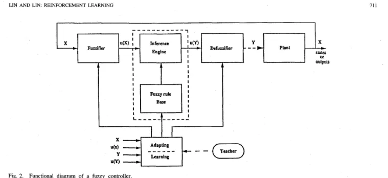
TeacherFig. 2. Functional diagram of a fuzzy controller.
connection types (fuzzy logic rules) for an RFALCON dynami- cally by means of an external reinforcement signal. Moreover, learning can proceed even before an external reinforcement feedback is available.
An important feature of the proposed leaming system is that it can dynamically partition the input-state space and output- control space using irregular fuzzy hyperboxes according to the distribution of environment states and reinforcement sig- nals. In many existing fuzzy or neural fuzzy control systems, including those introduced in the preceding paragraphs, the input and output spaces are always partitioned into “grids,” each defining a fuzzy region. The overlapping regions between the grids provide a smooth and continuous membership out- put surface. Consider, for example, a fuzzy logic controller with two input variables. If each of them contains three fuzzy terms (e.g., “small,” “medium,” and “large,”) then the corresponding input-space partition is as shown in Fig. l(a). Although during the learning process, the position and shape of membership functions will be changed, they are still inherently grid-type partitions. Due to its simplicity and intuitiveness, grid-type partitioning of input and output spaces has been used in the design of many existing fuzzy systems. As the number of input-output variables increases, however, the number of partitioned grids grows combinatorially. As a result, the memory or hardware size required may become impracticably large. This results in more learning difficulty since with finer space partitioning, more training samples are needed or insufficient leaming takes place. To avoid combinatorial growth of partitioned grids in complex systems, more flexible and irregular space partitioning methods must be developed. Fig. l(b) shows a proposed partitioning method in the RFALCON system. The problem of space partitioning from numerical training data is basically a clustering problem. The proposed system applies the fuzzy adaptive resonance theory (fuzzy ART) proposed by Carpenter et al. [24], [25] to do fuzzy
clustering in the input-output spaces and find proper fuzzy logic rules dynamically by associating input clusters with output clusters. The backpropagation learning scheme is then
used for tuning input-output membership functions. Hence, in the RFALCON, the fuzzy ART is used for structure learning and the backpropagation algorithm for parameter learning. The RFALCON can thus on-line partition the input-output spaces, tune membership functions, and find proper fuzzy logic rules dynamically on the fly. More notably, in this learning scheme, only the reinforcement signals from the outside world need to be provided. Users do not need to give the initial fuzzy partitions, membership functions, or fuzzy logic rules, hence, there are no hidden nodes at the beginning of learning; they are created and begin to grow as the first reinforcement signal arrives.
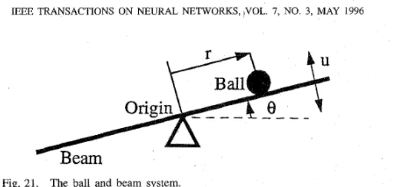
This paper is organized as follows: Section 11 describes the basic structure and functions of our previously proposed FALCON [ 2 ] . The proposed RFALCON and the correspond- ing reinforcement structure/parameter-learning algorithm with multistep prediction capability are presented in Section 111. In Section IV, the cart-pole balancing system and the ball and beam system are simulated to demonstrate the ability of the proposed RFALCON. Performance comparison with some other existing systems is described in Section V. Finally, conclusions are summarized in Section VI.
11. THE STRUCTURE OF THE FALCON
We shall briefly introduce basic components of conventional fuzzy control systems (for more details, please refer to [26]
and [27]), and then propose our connectionist model.
A. Basic Structure of A Fuzzy Control System
Fig. 2 shows the basic structure of a conventional fuzzy control system with a learning/adapting component. Before proceeding, we must define some important terms. A fuzzy set F in a universe of discourse U is characterized by a membership function p . ~ : U i [0,1]. Thus, a fuzzy set F in U may be represented as a set of ordered pairs. Each pair
consists of a generic element U and its grade of membership
function p ~ ( u ) ; that is, F = { ( U , ~ . F ( u ) )
I
U E U } . U is called a support value if ~ F ( u )>
0. If U is a continuous universe and712 IEEE TRANSACTIONS ON NEURAL NETWORKS, VOL. 7, NO. 3, MAY 1996
F is normal and convex (i.e., maxpF(u) = 1 and p ~ ( X u 1
+
then F is a fuzzy number. A linguistic variable x in a universe of discourse U is characterized by T ( x ) = {T:, T,,
. . .
,
T t }and M ( z ) = { M ; , M z , .
. .
) M t } , where T ( x ) is the term setof z; that is, the set of names of linguistic values of z with each value Ti being a fuzzy number with membership function
M i defined on U . So M ( z ) is a semantic rule for associating with each value its meaning. For example, if x indicates speed, then T ( z ) may be {slow, medium, fast}. Following the above definition, the input vector X which includes the input state
linguistic variables x,’s, and the output state vector Y which
includes the output state linguistic variables yz’s in Fig. 2 can be defined as
X =
U E U
(1 - X ) u 2 ) 2 m i n ( P F ( u l ) , P F ( U 2 ) ) , u1,u2 E
u>x
E [O,111,
{
(xz,
U%, {T,1$ > T:”,,
* * * ,T:;1
> {M:%,
@% >. . .
> M:: }1
Id,. 72)(1)
Y =
{(YZ,U,’, { T ~ ~ , T ~ ~ > . ’ . , T ~ ~ } , { M ~ ~ , M ~ ~ , . . . , M ~ } ) 12=1,.. , m > .
(2) The fuzzifier in Fig. 2 is a mapping from an observed input space to fuzzy sets in certain input universe of discourse. So a specific value x z ( t ) at time t is mapped to the fuzzy set T:%
with degree M 2 , ( x z ( t ) ) and to the fuzzy set T:% with degree
M:%(z%(t)), and so on.
The fuzzy rule base in Fig. 2 contains a set of fuzzy logic rules R. For a multi-input and multioutput (MIMO) system, we have
2
R { R L I . w o , R M I M O , . . .
,
R ~ M I M O1
where the zth fuzzy logic rule is
RLIncro
: IF ( z1 is T,, and. . .
and x p is T., ) THEN ( y1 is Tyl and and y4 is Tyn ). The preconditions ofR L I M o
form a fuzzy set T,, x. . .
x T.,and the consequent of R b I M O is the union of q independent outputs. So the rule can be represented by a fuzzy implication
R h I M O : (Tz, x . .
.
x T Z p ) + (Tyl+
.
. .+
Ty,) where“+”
represents the union of independent variables. Since the outputs of MIMO rule are independent, the general rule structure of MIMO fuzzy system can be represented as a collection of multi-input and single-output (MISO) fuzzy systems by decomposing the above rule into q subrules with Ty, as the single consequent of the ith subrule. For clarity,we shall consider MISO system in the following analysis. A sample rule follows:
IF the speed is too slow and the acceleration is decreasing, THEN increase power strongly.
The inference engine in Fig. 2 matches the rule precondi- tions in the fuzzy rule base with the input state linguistic terms and performs implication. For example, if there were two rules:
R1: IF x1 is T21 and x2 is T i 2 , THEN y is Tt.
R2: IF X I is T:, and x2 is T:2, THEN y is T i .
Then the firing strengths of rules R1 and R2 are defined as 01 and 122, respectively. Here a; is defined as
a, = K 1 ( x 1 ) A M:&2) ( 3 ) where ‘‘A“ is the fuzzy AND operation. The most commonly used fuzzy AND operations are intersection and algebraic product [26], [27].
Rules R1 and R2 lead to the corresponding decision with the membership function, f i i ( w ) , i = 1 , 2 , which is defined as
k ; ( w ) = at A M;(w) (4) where w is the variable that represents the membership func- tion support values. Combining these decisions, we obtain the output decision
f i y ( w ) = & i ( W )
v
k ; ( w ) ( 5 ) where “V“ is the fuzzy OR operation. The most commonly used fuzzy OR operations are union and bounded sum [25],W I .
Notice that the last result is a membership function curve. Before feeding the signal to the plant, we must defuzzify it to get a crisp decision, which is what defuzzifier block in Fig. 2 does. Among commonly used defuzzification strategies, the center of area method yields a superior result [26], [27]. Let
wJ be the support value at which the membership function,
Mi
( w ) , reaches the maximum value2;
( w )I
2u=w3.
Then thedefuzzification output is
- p ; ( w j ) w j
The preceding describes the standard function operations in a conventional fuzzy control system, although there are some alternatives for fuzzy OR, fuzzy AND, and reasoning operations [26], [27].
Most system designers usually chose their membership functions empirically and constructed fuzzy logical rules sup- plied by experts. Enabling fuzzy control systems to learn is an important issue. The learningladapting block in Fig. 2 represents this function. This leaming/adapting block finds suitable fuzzy logic rules and adapts the fuzzifier and the defuzzifier to find the proper shapes and membership function overlaps by learning the desired output, or in response to external reinforcement signals. The aim of this paper is to present an adaptive fuzzy control system design that can adapt itself in response to external reinforcement signals. In the next section, the FALCON, a connectionist model, is proposed as just such a fuzzy control system. This neural-network-based architecture eliminates the rule-matching process and distribu- tively stores control knowledge in the connection types and link weights. More importantly, the connectionist architecture is a natural structure with which to perfom neural-network- based learning.
LIN AND L I N REINFORCEMENT LEARNING 713
Joint-1 Tracking Error Joint-2 Trackinq Error
0 0 2 0 02
-
E 0 01I
P o 01 D-
P 0 g 5 - 0 “ 0 0 I 4 E ago
01 E-0 01 .a 7 ? 0 0 2 0 02 0 03 U 1 5 10 15 20 -0 03 Time (seconds)b
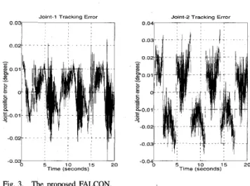
5 10 1 5 20 -004; Time (seconds)Fig. 3. The proposed FALCON.
B. A Connectionist Fuzzy Control System
In this section, we shall describe the structure and functions of the proposed FALCON [2], a connectionist realization of a conventional fuzzy logic control system and also a basic component of the proposed RFALCON, that will be introduced in Section 111. The FALCON system (see Fig. 3) has five layers with node and link numbering defined by the brackets on the right-hand side of the figure. Layer-1 nodes are input nodes (input linguistic nodes) representing input linguistic variables. Layer-5 nodes are output nodes (output linguistic nodes) repre- senting output linguistic variables. Layer-2 and layer-4 nodes are term nodes that act as membership functions representing the terms of the respective input and output linguistic variables. Each layer-3 node is a rule node representing one fuzzy logic rule. Thus, together all the layer-3 nodes form the fuzzy rule base. Links between layers 3 and 4 function as a connectionist inference engine. Layer-3 links define the preconditions of the rule nodes, and layer-4 links define the consequents of the rule nodes. Therefore, each rule node has at most one link to some term node of a linguistic node, and may have no such links. This is true both for precondition links (links in layer 3 ) and consequent links (links in layer 4). The links in
layers 2 and 5 are fully connected between linguistic nodes and their corresponding term nodes. The arrows indicate the normal signal flow directions when the network is in operation (after it has been built and trained). We shall later indicate the signal propagation, layer-by-layer, according to the arrow direction.
The FALCON uses the technique of complement coding from Fuzzy ART [24] to normalize the input-output training vectors. Complement coding is a normalization process that rescales an n-dimensional vector in
X2”,
x = (21, x 2 ,,
xn),to its 2n-dimensional complement coding form in [O, 1Izn, x’, such that
x’ (51,
z;,
3 Z 7z;,
.
..
z,,
3;) (7)= (31,l- 3 1 , 2 2 , 1 - 3 2 ,
where ( f l , Z z , .
.
.
, 2 , ) = X = x/11x11 and 37 is the com- plement of 3 1 , i.e., 3; = 1 - 3 1 . As mentioned in [24], complement coding helps avoid the problem of category proliferation when using fuzzy ART for fuzzy clustering. It also preserves training vector amplitude information. Inapplying the complement coding technique to the FALCON, all training vectors (either input state vectors or desired output vectors) are transformed to their complement coded forms in the preprocessing process, and the transformed vectors then used for training.
A typical network consists of nodes with some finite number of fan-in connections from other nodes represented by weight values, and fan-out connections to other nodes. Associated with the fan-in of a node is an integration function f which
combines information, activation, or evidence from other nodes, and provides the net input; i.e.,
where zZ(‘) is the ith input to a node in layer
k,
and is the weight of the associated link. The superscript in the above equation indicates the layer number. This notation will be also used in the following equations. Each node also outputs an activation value as a function of its net-inputoutput = a( f ) (9) where a(.) denotes the activation function. We shall next describe the functions of the nodes in each of the five layers of the FALCON. Assume that the dimension of the input space is n, and that of the output space is m.
Layer 1: Each node in this layer is called an input linguistic node and corresponds to one input linguistic variable. Layer- 1 nodes just transmit input signals to the next layer directly. That is
f ( ~ Z , z ~ ) = ( ~ z , ~ : , C ) = ( ~ , , l - ~ z ) a n d a ( f ) = f . (10) From the above equation, the link weight in layer 1 (w:’)) is unity. Noted that due to the complement coding process, for each input node i, there are two output values, 3, and
Layer2: Nodes in this layer are called input term nodes
and each represents a term of an input linguistic variable, and acts as a one-dimensional membership function. The following trapezoidal membership function [3 11 is used:
x; = 1 - 3,.
and
4.f)
=f
where and U!:) are, respectively, the left-flat and right-
flat points of the trapezoidal membership function of the jth input term node of the ith input linguistic node [see Fig. 4(a)];
z$) is the input to the j t h input term node from the ith input linguistic node (i.e., z$) = 5&); and
1 if sy
>
1{
0 if sy<
0.g(s,y) = sy if 0
5
sy5
1 (12)The parameter y is the sensitivity parameter that regulates the fuzziness of the trapezoidal membership function. A large y means a more crisp fuzzy set, and a smaller y makes the fuzzy set less crisp. A set of n input term nodes (one for each
714 IEEE TRANSACTIONS ON NEURAL NETWORKS, VOL. 7, NO. 3, MAY 1996 1 I 0 . Membership value 0. (b)
Fig. 4. (a) One-dimensional trapezoidal membership function. @)
Two-dimensional trapezoidal membership function.
input linguistic node) is connected to a rule node in layer 3 where its outputs are combined. This defines an n-dimensional membership function in the input space, with each dimension specified by one input term node in the set. Hence, each input linguistic node has the same number of term nodes. That is, each input linguistic variable has the same number of terms in the FALCON. This is also true for output linguistic nodes. A layer-2 link connects an input linguistic node to one of its term nodes. There are two weights on each layer-2 link. We denote the two weights on the link from input node i (corresponding to the input linguistic variable z,) to its j t h term node as
U!,”’ and U!,“’ (see Fig 3). These two weights define the correspond respectively to the two inputs, 8, and’;,“ from the input linguistic node
i.
More precisely, x, and Zc,“, the two inputs to the input term node j , will be used during the fuzzy- ART clustering process in FALCON’S structure-learning step to decide U::) and U::), respectively. In FALCON’S parameter- learning step and normal operating, only 8% is used in the forward reasoning process [i.e., 2::) = 8, in (ll)]. We detail the FALCON learning scheme in Section 111.Layer 3: Nodes in this layer are called rule nodes and each
represents one fuzzy logic rule. Each layer-3 node has n input membership function in (11). The two weights, u ( ~ ) and vZJ (2) ,
term nodes, fed into it,’ one for each input linguistic node. Hence, there are as many rule nodes in the FALCON as there are term nodes of an input linguistic node (i.e., the number of rules equals the number of terms of an input linguistic variable). Notice that each input linguistic variable has the same number of terms in the FALCON as mentioned in the above. The links in layer 3 are used to perform precondition matching of fuzzy logic rules. Hence the rule nodes perform the following operation
n
i=l
where z2(3) is the ith input to a node in layer 3 and the
summation is over the inputs of this node. The link weight in layer 3
(~2”’)
is then unity. Note that the summation in the above equation is equivalent to defining a multidi- mensional (n-dimensional) membership function, which is the summation of the trapezoid functions in (11) over i . This forms a multidimensional trapezoidal membership function called the hyperbox membership function [31], since it is defined on a hyperbox in the input space. The corners of the hyperbox are decided by the layer-2 weights, U::) and v!”, for all 2’s. More clearly, the interval [u!:),u!$)~ defines t G edge of the hyperbox in the ith dimensTon. Hence, the weight vector, [(urf’ ) vis’), .. .
,
(U::’, U::))). . .
,
(U$), U:))],defines a hyperbox in the input space. An illustration of a two-dimensional hyperbox membership function is shown in Fig. 4(b). The rule nodes output are connected to sets of m output term nodes in layer 4, one for each output linguistic variable. This set of output term nodes defines an m-dimensional trapezoidal (hyperbox) membership function in the output space that specifies the consequent of the rule node. Note that different rule nodes may be connected to the same output hyperbox (i.e., they may have the same consequent), as is shown in Fig. 3.
Layer4: The nodes in this layer are called output term
nodes; each has two operating modes: down-up transmission and u p d o w n transmission modes (see Fig. 3). In down-up transmission mode, the links in layer 4 perform the fuzzy OR operation on fired (activated) rule nodes that have the same consequent
where 2,’“’ is the zth input to a node in layer 4 and p is the number of inputs to this node from the rule nodes in layer 3. Hence the link weight = 1. In up-down transmission mode, the nodes in this layer and the up-down transmission links in layer 5 function exactly the same as those in layer 2: each layer-4 node represents a term of an output linguistic variable and acts as a one-dimensional membership function. A set of m output term nodes, one for each output linguistic node, defines an m-dimensional hyperbox (membership function) in the output space, and there are also two weights, U::) and U::’, on each of the up-down transmission links in layer 5 (see Fig. 3). The weights define hyperboxes (and thus the associated hyperbox membership
LIN AND LIN REINFORCEMENT LEARNING 715
Joint-1 Tracking Error Joint-2 Tracking Error
0.15, I I I
0 5 10 15 20 Time (seconds) -0.15 0 5 10 15 20 -0.1
Time (seconds)
Fig. 5. The fuzzy reasoning process in the FALCON model.
functions) in the output space. More clearly, the weight defines a hyperbox in the output space.
Layer 5: Each node in this layer is called a output linguistic node and corresponds to one output linguistic variable. There are two kinds of nodes in layer 5. The first kind of node performs up-down transmission for training data (desired outputs) to feed into the network, acting exactly like the input linguistic nodes. For this kind of node, we have
(15) where
9,
is the ith element of the normalized desired output vector. Notice that complement coding is also performed on the desired output vectors. Thus, as mentioned above, there are two weights on each of the up-down transmission links in layer 5 (the U::) and us’ shown in Fig. 3). The weights definehyperboxes and the associated hyperbox membership functions in the output space. The second kind of node performs down- up transmission for decision signal output. These nodes and the layer-5 down-up transmission links attached to them act as a defuzzifier. If U$) and U::’ are the corners of the hyperbox of the j t h term of the 2th output linguistic variable y,, then the following functions can be used to simulate the center of area defuzzification method:
vector, [(U!:), vi:)),
. . .
,
(U::), v!:)),. . .
,
(umg, ( 5 ) vm,)], ( 5 )f(Y,,Y,“)
= ( Y Z , Y P ) = (Yz, 1- YJ
and a ( f ) =f
where zi5’ is the input to the 2th output linguistic node from its j t h term node, and m::) = (U::’
+
v::))/2 denotes the centervalue of the output membership function of the j t h term of the ith output linguistic variable. The center of a fuzzy region is defined as that point with the smallest absolute value among all the other points in the region at which the membership function membership value is equal to one. Here the weight, tu$’), on a down-up transmission link in layer 5 is defined the weights on the corresponding up-down transmission link in layer 5 .
by w,, ( 5 ) = - mz,, ( 5 ) = (U::)
+
vi:))/2, where U$’ and U$) x eThe fuzzy reasoning process in the FALCON is illustrated in Fig. 5, which shows a graphic interpretation of the center of area defuzzification method. Here, we consider a two-input and two-output case. As shown in the figure, three hyperboxes (IH1, IH2, and IH3) are formed in the input space and two hyperboxes (OHl,OH2) are formed in the output space. These hyperboxes are defined by the weights ut3, vzg, U:,, and U:,.
The three fuzzy rules indicated in the figure are “IF x is
IHl THEN y is OH1 (rule l),” “IF x is IH2 THEN y is OH1 (rule 2),” and “IF x is IH3 THEN y is OH2 (rule 3),”
where x = ( x 1 , ~ ) and y = (y1,yz). If an input pattern is located inside a hyperbox, the membership value is equal to one [see (12)]. In this figure, according to (14), z1 is obtained by performing fuzzy OR (maximum) operation on the inferred results of rules 1 and 2, which have the same consequent, OH1. Also according to (14), z2 is directly the inferred result of rule 3. z1 and z~ are then defuzzified to get the final output according to ( 16).
Note that with the proposed learning algorithms developed in Section 111, no input-output term nodes and no rule node are presented when learning begins. They are created dynamically as on-line teaching signals are received and learning proceeds. In other words, the FALCON initially has only input and output linguistic nodes before training, other input and output term nodes and rule nodes are added during the learning process.
An on-line supervised learning algorithm originally pro- posed in [2] is associated with the FALCON to perform on-line training. This algorithm works very well when supervised training data are available on-line, however, it requires precise training data to indicate the exact desired outputs, and to compute the output errors for training the whole network. Unfortunately, such detailed and precise training data may be very expensive or even impossible to obtain in some real- world applications because the controlled system may only be able to provide the learning algorithm with a reinforcement signal such as a binary right-wrong decision from the current controller. Thus, we propose two FALCON’s integrated into a structure called RFALCON to train networks with this kind of evaluative feedback. The RFALCON and an associated reinforcement learning algorithm are presented in the next section.
111. LEARNING ALGORITHM FOR THE RFALCON WITH A MULTISTEP CRITIC NETWORK
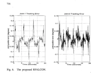
This section presents details of the integrated RFALCON network and associated learning algorithm we propose. The RFALCON consists of two FALCON’S, one of which is used as an action network, and the other as a critic network (see Fig. 6). The reinforcement learning algorithm combines structure learning and parameter learning to determine the proper corners of the hyperbox (uo’s and v,j’s) for each
term node in layers 2 and 4. It also learns fuzzy logic rules and link connection types in layers 3 and 4; that is, the precondition and consequent links of the rule nodes. All the learning is performed on both FALCON’s simultaneously and only conducted by a reinforcement signal feedback from the external environment. Unlike the supervised learning problem
116
Joint-1 Tracking Error
0.251 ~ I
Fig. 6 . The proposed RFALCON.
Joint-2 Tracking Errol
_ _
in which the correct “target” output values are given for each input pattern to instruct network learning, the reinforcement learning problem has only very simple “evaluative” or “critic” information available for learning rather than “insmctive” information. In the extreme case, there is only a single bit of information to indicate whether the output is right or wrong. Fig. 6 shows how a network and its training environment interact in a reinforcement learning problem. The environment supplies a time-varying input vector to the network, receives its time-varying output-action vectors, and then provides a time-varying scalar reinforcement signal. In this paper, the reinforcement signal r ( t ) is two-valued, r ( t ) E { - l , O ) , such that r ( t ) = 0 means “a success” and r ( t ) = -1 means “a failure.” We also assume that r ( t ) is the reinforcement signal available at time step t and is caused by the inputs and actions chosen at earlier time steps (i.e., at time steps
t - 1, t - 2,
. .
.). The goal of learning is to maximize a function of this reinforcement signal, such as the expectation of its value on the upcoming time step or the expectation of some integral of its values over all future time.The precise computation of the external reinforcement sig- nal is highly dependent on the nature of the environment and is assumed to be unknown to the learning system. It could be a deterministic or stochastic function of environment states and network outputs. In most cases, the environment is itself governed by a complicated dynamic process, in which reinforcement signals and input patterns may depend on past network outputs. In a chess game, for example, the environment is actually another player, and the network only receives a reinforcement signal (win or lose) after a long sequence of moves.
To resolve this class of reinforcement learning problems, a system, called the RFALCON, is proposed. Associated with the RFALCON is a reinforcement structure/parameter- learning algorithm. As Fig. 6 shows, the proposed RFALCON consists of two FALCON’S: one FALCON for the action network (fuzzy controller) and the other FALCON for the critic network (fuzzy predictor). Each network has exactly the same structure as shown in Fig. 3. The action network can have multiple outputs as shown in Fig. 3, although only one output node is shown in Fig. 6. In the multioutput case, all the output nodes of the action network receive the same internal
IEEE TRANSACTIONS ON NEURAL. NETWORKS, VOL. 7, NO. 3, MAY 1996 reinforcement signals from the critic network, which has only one output node since it is used to predict the external scalar reinforcement signal. Since we want to solve reinforcement learning problems in which the external reinforcement signal is available only after a long sequence of actions have been passed on to the environment, we need a multistep critic network to predict the external reinforcement signal. The action network decides a best action to impose onto the environment in the next time step according to the current environment status and predicted reinforcement signals. The critic network models the environment such that it can perform a multistep prediction of the reinforcement signal that will eventually be obtained from the environment for the current action chosen by the action network. The multistep predicted reinforcement signal thus enables both the action network and the critic network to learn at each time step without waiting for the arrival of an external reinforcement signal, greatly accelerating the learning of both networks.
In this section, we introduce the proposed reinforcement structure/parameter-learning algorithm for the WALCON with a multistep critic network. We first consider the reinforcement structure/parameter-learning scheme for the multistep critic network and then introduce the reinforcement learning scheme for the action network.
A. The Multistep Critic Network
We shall use a FALCON to develop a multistep critic network that can perform multistep prediction of an external reinforcement signal. When both the reinforcement signal and input patterns from the environment depend arbitrarily on the past history of the action network outputs and the action network only receives a reinforcement signal after a long sequence of outputs, the credit assignment problem becomes severe. This temporal credit assignment problem results because we need to assign credit or blame to each step individually in long sequences leading up to eventual successes or failures. Thus, to handle this class of rein- forcement learning problem, we need to solve the temporal credit assignment problem along with solving the original structural credit assignment problem concerning attribution of network errors to different connections or weights. The solution to the temporal credit assignment problem we propose in the RFALCON is including a multistep critic network that predicts the reinforcement signal at each time step in a given period without any external ,reinforcement signals from the environment. This will ensure that both the critic network and the action network can both update their parameters and structures during the period without any evaluative feedback from the environment. To solve the temporal credit assignment problem, we used a technique based on the temporal-difference method, which is often closely associated with dynamic pro- gramming techniques [12], [16], [29]. Unlike the single-step prediction and the supervised learning methods which assign credit according to the difference between the predicted and actual outputs, the temporal-difference methods assign credit according to the difference between temporally successive predictions. Notice that the term “multistep prediction” used here means the critic network can predict a value that will
LIN AND LIN: REINFORCEMENT LEARNING
process
717
Mapping Process
Gayer
3)
be available several time steps later, although it does such prediction at each time step to improve its prediction accuracy. In this paper, we consider the case of infinitely discounted predictions [16], [20]. In this case, the critic network output, pt- 1, predicts accumulatively discounted outcomes (external reinforcement signals)
Cy=o
tkrt+r, = r t+
t p t , where pt-1 is the output of the critic network at time t - 1, rt is the actual outcome occurring between time stepst
- 1 andt,
and the discount-rate parameterE ,
05
<
1, determines the extent to which we are concerned with short- or long-range predictions. Since the actual outcome (external reinforcement signal), r t ,is not available at each time step in the problems we consider,
r t is set to zero during the period when there is no external reinforcement signal. The actual external reinforcement signal may be available at some unexpected time long after time step t - 1. The infinitely discounted prediction is used for
prediction problems in which exact success or failure may never be completely known. In this case, the prediction error is (rt
+
[ p t ) - pt-l, and the learning rule ist-1
Awt = v ( r t
+
t p t - pt-I) Xt-k-lVwpli (17) where w represents the adjustable network parameter (weight),v
is the learning rate, and X is the recency weighting factor with which weight update due to the predictions of observation vectors occurring k steps in the past are weighted byXk.
In applying the temporal difference procedures to the proposed RFALCON, we let X = 0 for efficiency and accuracy [16]. A general learning rule used for infinite discounted predictions is thusk = l
We shall next derive the learning rule for the multistep critic network according to (18). Here, p ( t )
=
pt is the single output of the critic network for the network‘s current parameter, w(t), and current given input state vector,z ( t ) ,
at time stept.
According to (18), let
+(t) = ~ ( t )
+
@(t) - p ( t - 1), 01.
<
<
1. (19)Then
+(t)
is the multistep critic network’s output node error signal. With the (predicted) desired output, p ( t ) , and theoutput error signal, +(t), available, we can use the supervised learning techniques to train the critic network. Note that if the environment provides a reinforcement signal at each time step, the critic network can “single-step,’’ or calculate the actual learning output error at each time step. Thus, the critic network can operate as either a multistep or single-step predictor.
Thus far, we have formulated the multistep prediction problem as a supervised learning problem, so the on-line learning algorithm proposed in [ 2 ] can be adopted directly here. This learning scheme uses the fast-learn fuzzy ART for structure learning and the backpropagation algorithm for parameter learning of each incoming training pattern. When learning begins, only input and output linguistic nodes are presented, and user need not provide fuzzy partitions, mem-
Input
Training Data
7-
Prediction
Input Space
Partition Process
Vigilanc
Layer 2
OutputSpace
Partition Process
Layer 5
Vigilanc
I
Layer
4+Parameter Learning
(Hyperbox Tuning)
Fig. 7. Flowchart of the proposed reinforcement structure/parameter- learning algorithm.
bership functions, and fuzzy logic rules. As training data are received, input and output term nodes, and rule nodes are created dynamically. Then as learning proceeds, more are added as they are needed.
We present the reinforcement learning algorithm for the critic network in detail in the rest of this section. A flowchart of
this reinforcement learning algorithm is shown in Fig. 7. Basi- cally, we use the temporal difference prediction method to find the output error of the critic network. The error is then used for training the critic network by the proposed reinforcement learning algorithm. This learning algorithm consists of two steps: the structure-learning step and the parameter-learning step, as introduced in the following two sections, respectively.
1 ) The Structure-Learning Step: The structure-learning task can be stated as: Given input training data at time t , z z ( t ) , i = 1,
. . ,
n and desired output value r ( t ) , we need proper fuzzy partitions, membership functions, and fuzzy logic rules. At this stage, the network works in a two-sided manner; that is, the718 IEEE TRANSACTIONS ON NEURAL NETWORKS, VOL. I, NO. 3, MAY 1996 nodes and links in layer 4 are in the up-down transmission
mode so training input and output data are fed in from both sides.
The structure-learning step consists of three learning pro- cesses: input fuzzy clustering process, output fuzzy clustering process, and mapping process. The first two processes are performed simultaneously on both sides of the network, and are described below.
a ) Input Fuzzy Clustering Process: We use the fuzzy
ART fast learning algoritha [24,25] to find the input membership function parameters, U::’ and
‘ujf).
This isequivalent to finding proper input space fuzzy clustering or, more precisely, to forming proper fuzzy hyperboxes in the input space. Initially, for each complement coded input vector x’ [see (7)], the values of choice functions, T3, are
computed by
where “ A ” is the minimum operator performed for the pair- wise elements of two vectors, a!
>
0 is a constant, N isthe current number of rule nodes, and wj is the comple- ment weight vector, which is defined by - wi i(u, _ . ( 2 ) - 3
,
1 -‘ulj),...,(uij (2) ( 2 ) , 1 - U,$)), . . . , ( u$),l -
‘us))].
Notice that [ ( U ! ; ) , U!:’),.
,
(u.. 2 3 (2)’
‘u.. 2 3 (2) ),. . .
,
(unj ( 2 ),
‘unj (2) )] is the weight vector of layer-2 links associated with rule node j. The choice function value indicates the similarity between the input vectorx‘ and the complement weight vector w3. We then need to find the complement weight vector closest to x’. This is equivalent to finding a hyperbox (category) that x’ could belong to. The chosen category is indexed by J , where
Resonance occurs when the match value of the chosen cate- gory meets the vigilance criterion
where p E [0,1] is a vigilance parameter. If the vigilance criterion is not met, we say mismatch reset occurs. In this case, the choice function value TJ is set to zero for the duration of
the input presentation to prevent persistent selection of the same category during search (we call this action “disabling J “ ) . A new index J is then chosen using (21). The search process continues until the chosen J satisfies (22). This search
process is indicated by the feedback arrow marked with “vigilance test“ in Fig. 7. If no such J is found, then a new
input hyperbox is created by adding a set of n new input term
nodes, one for each input linguistic variable, and setting up links between the newly added input term nodes and the input linguistic nodes. The complement weight vectors on these new layer-2 links are simply given as the current input vector, x’. These newly added input term nodes and links define a new hyperbox, and thus a new category, in the input space. We denote this newly added hyperbox as J .
b) Output Fuzzy Clustering Process: The output fuzzy clustering process is exactly the same as the input fuzzy clustering process except that it is performed between layers 4 and 5 which are working in the up-down transmission mode. Of course, the training pattern used now is the desired output vector after complement coding, r/ = (T, T c ) = (T, 1 - T).
We denote the chosen or newly added output hyperbox by
K . This hyperbox is defined by the complement weight vector in layer 5, WK = [(Ul3 ( 5 ) , I - v@’),
. . .
,
(Uz3 ( 5 ),
I - va3 ( 5 )>,
. . . , ( U:;, 1 -.3].
The two fuzzy clustering processes above produce a chosen input hyperbox indexed as J and a chosen output hyperbox indexed as K , where the input hyperbox J is defined by WJ and the output hyperbox K by W K . If the chosen input hyperbox J is not newly added, then there is a rule node, J ,
that corresponds to it. If the input hyperbox J is a newly added one, then a new rule node (indexed as J ) in layer 3 is added, and connected to the input term nodes that constitute it.
e) Mapping Process: After the two hyperboxes in the in-
put and output spaces are chosen in the input and output fuzzy clustering processes, the next step is to perform the mapping process which decides the connections between layer-3 and layer-4 nodes. This is equivalent to deciding the consequents of fuzzy logic rules. This mapping process is described by the following algorithm, wherein connecting rule node J to output hyperbox K we means connecting the rule node J to the output term nodes that constitutes the hyperbox K in the output space.
Step 1) IF rule node J is a newly added node
THEN connect rule node J to output hyperbox K.
Step 2) ELSE IF rule node J is not connected to output hyperbox K originally
THEN disable J and perform input fuzzy clustering process to find the next qualified J [i.e.,
the next rule node that satisfies (21) and (22)]. Go to Step 1).
Step 3) ELSE no structure change is necessary.
In the mapping process, hyperboxes J and K are resized
according to the fast learning rule [24] by updating weights,
W J and W K , as follows:
Note that once the consequent of a rule node has been decided in the mapping process, it will not be changed thereafter. We now use Fig. 5 to illustrate the structure- learning step as follows. For a given training datum, the input fuzzy clustering process and the output fuzzy clustering process find or form proper clusters (hyperboxes) in the input and output spaces. Assume that the input and output hyperbox pair found (or formed) are ( J , K ) . The mapping process then tries to relate these two hyperboxes by setting up links between them. This is equivalent to finding a fuzzy logic rule that defines the association between an input hyperbox and an output hyperbox. If this association exists already (e.g., ( J , K )
= (IH1, OHl), (IH2, OHl), or (IH3, OH2) in Fig. 5), then no structural change is necessary. If input hyperbox J is
LIN AND LIN REINFORCEMENT LEARNING 719 newly formed and thus not connected to any output hyperbox,
it is connected to output hyperbox K directly. Otherwise,
different from K originally (e.g., ( J , K ) = (IH2, OH2)), then
then easily derived
if input hyperbox J is associated with an output hyperbox zz p ( t - 1) - ~ ( t ) - e p ( t ) = -?(t) (25)
a new input hyperbox close to J will be found or formed
by performing the input fuzzy clustering process again. This search, called “match tracking” (see Fig. 7), continues until an input hyperbox, J‘, that can be associated with output hyperbox K is found [e.g., ( J ’ , K ) = (IH3, OH2)].
The vigilance parameter, p , is an important structure- learning parameter that determines learning cluster density. High (approaching one) p values tend to produce increasingly finer learning clusters, until at one, each training datum is assigned to its own cluster in the input (output) space. Low (approaching zero) p values tend to produce increasingly coarser learning clusters, until at zero, all training data are assigned to a single cluster in the input (output) space.
Clearly, a constantly high or low p value will result in
formation of excessively high numbers of clusters on the one hand, or very low output accuracy (and thus, low network representation power) on the other hand. For these reasons, we chose an adaptive vigilance strategy in which the p parameter is initially set high to allow fast RFALCON structure growth, and then monotonically decreased to slow cluster formation and stabilize learning. Empirical studies have shown this approach to be efficient and stable in the learning speeds and numbers of clusters it produces.
2 ) The Parameter-Leaming Step: After the network struc-
ture has been adjusted according to the current training pattern in the structure-learning step, it is then necessary to fine tune the network parameters using the same training pattern. This fine tuning process is necessary to assure the desired output accuracy of a network for controUprediction problems. Using the terminology of fuzzy logic: once our fuzzy controller has found its fuzzy logic rules, its membership functions must be tuned to make its output meet the desired output as closely as possible. Notice that the following parameter learning is performed on the whole network after structure learning, no matter whether the nodes (links) are newly added or are existent originally. The parameter-learning task can be stated as: Given the training input data xt(t), i = 1,
. . .
,
n,the desired output value, and the network structure (specified by input and output hyperboxes and fuzzy logic rules), we need to adjust the network parameters to make the network output match the desired output values as closely as possible. Thus, the network works in a feedforward manner; that is, the nodes and links in layer 4 are in the down-up transmission mode. Basically, the backpropagation algorithm is used to find node output errors, which are then analyzed to guide parameter adjustment.
The goal of training the multistep critic network is to minimize the error function [see (19)]
1
2
E = - ( ~ ( t )
+
J p ( t ) - ~ ( t -where
~ ( t )
is the actual external reinforcement signal, and p ( t )is the predicted reinforcement signal. Gradient information is
where the subscript
t
- 1 represents the time displacement. The time displacement in (25) and the remaining equations in this paper reflect the assumption that the reinforcement signal (which may be the “predicted” reinforcement signal) at time stept
depends on the input state and chosen action at time step t - 1.We can derive the structure/parameter-learning algorithm for the multistep critic network using the following general parameter-learning rule:
d E
w ( t
+
1) = ~ ( t )+
A w ( t ) =~ ( t )
+
~ ( - d u ) ) , (26) (27) where w is the adjustable parameter in the critic network (i.e.,u;j or q j ) . The general parameter-learning rule then is
d E - dE a p
_ _ -
aw
apaw
A w ( t ) = r]?(t)
[
4
.
t-1
To show the parameter-learning rules, we derive the rules layer-by-layer using the hyperbox membership functions with corners uz3’s and vi3’s as the adjustable parameters for these computations. In the following derivation, we consider only one output linguistic variable for notational clarity. Hence, the adjustable parameters in layer 5 are denoted by U:), v:~), and
m y ) = (u:5)
+
~ : ~ ) ) / 2 , for the j t h term node.Layer 5: Using (16), (26), and (27), the updating rule for
the comers of the hyperbox membership function
~ 1 ~ )
isAnd the corner parameter is updated by
Similarly, using (16), (26), and (27), the updating rule for the other corner parameter u : ~ ) is
And the other corner parameter is updated by
720 IEEE TRANSACTIONS ON NEURAL NETWORKS, VOL 7, NO. 3, MAY 1996
Layer4: There is no parameter to be adjusted in this
layer. Only the error signal
(S,(“))
needs to be computed and propagated. According to (16), the error signal is deriveddE
- d E da(5) by(34) ($4) = --
da(4) - &(5) da(4) where
(35)
Hence, the error signal is
So the adaptive rule of w$) is
Similarly, using (1 l), (26), and (27), the updating rule of U:;)
is derived as
where
In the multioutput case, the computations in layers 5 and 4 are exactly the same as the above and proceed independently for each output linguistic variable.
computed in this layer. According to (14), this error signal can be derived by
Hence, the adaptive rule of uz3 becomes
u:;)(t
+
I) = u ! p ( t )+
$:3)[e]
.
The proposed reinforcement learning algorithm provides a novel on-line scheme to combine the structure and the param- eter learning such that they can be performed simultaneously.(50)
Layer 3: As in layer 4, only the error signals need to be
a u p
t--l (38) d E d a ( 4 ) - - d E
p
= - - -da(3) da(4) d f ( 4 ) da(3)
where B. The Action Network
~ - -s!4), d E da(4) -
ad4)
dfo
= 1, d f ( 4 ) d f ( 4 ) - 44) (39) (40) (41)In this section, we develop the reinforcement learning algorithm for the action network. The goal of this reinforce- ment structure/parameter-learning algorithm is to adjust the parameters (e.g., w’s) of the action network, to change the connection types, or even to add new nodes, if necessary, such that the reinforcement signal is maximum; that is
-
~~~ -
da(3) dz,(4) - Xmax
where z,,, = max(inpu1s of output terms node j ) . The term
z(4)
-
normalizes the error to be propagated for fired rules with the same consequent. Hence the error signal is z,,,If there are multiple outputs, then the error signal becomes
s ! 3 ) =
[ g ]
6f), where the summation is performed over the consequents of a rule node; that is, the error of a rule node is the summation of the errors of its consequents.Layer 2: Using ( l l ) , (26), and (27), the updating rule of
w!:) is derived as in the following: t-1 d E d a ( 3 ) da(’) (43) - d E - - - - _ _ _ ~ dw(2) - & (3) dWP) 2 3 23 where (44) dr
aw
K-.
dwTo determine
E,
we need to know%,
where g is the output of the action network. (For clarity, we discuss the single- output case first.) Since the reinforcement signal does not provide any hint as to what the right answer should be in terms of a cost function, there is no gradient information, and the gradient,E,
can only be estimated. If we can estimatee,
then the on-line supervised structurelparameter- learning algorithm developed in the last section for the critic network can be directly applied to the action network to solve the reinforcement learning problem. To estimate the gradient information in a reinforcement learning network, there needs to be some randomness in how output actions are chosen by the action network so the range of possible outputs can be explored to find a correct value. Thus, the output nodes (layer 5) of the action network are now designed to be stochastic units which compute their output as a stochastic function of their input.In our learning algorithm, the gradient information,