Computers Math. Applic. Vol. 31, No. 3, pp. 33-42, 1996
P e r g a m o n Copyright~)1996 Elsevier Science Ltd
Printed in Great Britain. All rights reserved 0898-1221/96 $15.00 + 0.00 0898-1221 (95) 0 0 2 0 4 - 9
A Parallel P o i s s o n G e n e r a t o r
U s i n g Parallel Prefix
T A N - C H U N
Lu,
Y u - S O N G H O U A N D R O N G - J A Y E C H E N * D e p a r t m e n t of Computer Science and Information EngineeringNational Chiao Tung University 1001 TA Hsueh Road Hsinchu 300, Taiwan, R.O.C.
rj chen@csie, n c t u . edu. tw
(Received May 1993; revised and accepted May 1995)
A b s t r a c t - - I n this paper, we use the renewal theory to develop a Poisson random number al- gorithm without restart. A parallel Poisson random number generator is designed based on this algorithm and prefix computation. This generator iteratively produces m Poisson random numbers with mean # in average time complexity O([mtt/n]f(n,p)) on EREW PRAM, where f(n,p) is the time for computing an n-element parallel prefix on p processors in each iteration, assuming that parallel uniform random numbers can be generated at the rate of one number per unit time per processor. If n is selected near mtt, it achieves linear speedup when p is small and the average time complexity is O(log(mp)) when p is O(mtt).
U e y w o r d s - - R a n d o m number generator, Poisson distribution, Parallel prefix computation.
1. I N T R O D U C T I O N
R e c e n t l y , m a n y u n i f o r m r a n d o m n u m b e r g e n e r a t o r s have b e e n p r e s e n t e d for p a r a l l e l m a c h i n e s . M a t t e i s a n d P a g n u t t i p a r t i t i o n e d a single p s e u d o - r a n d o m sequence a m o n g t h e a v a i l a b l e p r o c e s s o r s in [1] a n d u s e d one l i n e a r c o n g r u e n t i a l g e n e r a t o r for e a c h p r o c e s s o r in [2]. D e £ k [3] i m p l e m e n t e d G e n e r a l F e e d b a c k Shift R e g i s t e r ( G F S R ) for t h e C o n n e c t i o n m a c h i n e a n d t h e T series, w h i l e A l u r u et al. [4] u s e d G F S R o n p a r a l l e l c o m p u t e r s w h e r e t h e n u m b e r o f p r o c e s s o r s is a p o w e r o f two.
P o i s s o n d i s t r i b u t i o n r e p r e s e n t s t h e n u m b e r o f o c c u r r e n c e s p e r u n i t t i m e , a n d a n e v e n t c a n o c c u r a t a n y i n s t a n t o f t i m e . F o r e x a m p l e , t h e n u m b e r o f a l p h a p a r t i c l e s e m i t t e d b y a r a d i o a c t i v e s u b s t a n c e in a single second, o r t h e n u m b e r of a r r i v a l s in a n M / M / 1 Q u e u e in a single s e c o n d h a s a P o i s s o n d i s t r i b u t i o n . K n u t h [5] i n t r o d u c e d a s i m p l e s t o c h a s t i c m o d e l t o g e n e r a t e P o i s s o n r a n d o m v a r i a b l e s u s i n g e x p o n e n t i a l r a n d o m n u m b e r s . I n t h i s p a p e r , we p r e s e n t a new a l g o r i t h m t o g e n e r a t e P o i s s o n r a n d o m n u m b e r s , b a s e d o n u n i f o r m n u m b e r s . I n S e c t i o n 2, we d e s c r i b e t h i s s t o c h a s t i c m o d e l , a n d e x t e n d it t o g e n e r a t e m a n y P o i s s o n r a n d o m n u m b e r s . I n S e c t i o n 3, we i n t r o d u c e a p a r a l l e l P o i s s o n r a n d o m n u m b e r g e n e r a t o r . F i n a l l y , S e c t i o n 4 c o n c l u d e s t h e p a p e r w i t h a n o t e o n t h e p o s s i b l e p a r a l l e l m o d e l s of t h e P o i s s o n r a n d o m n u m b e r g e n e r a t o r .
The authors wish to thank the referee for his detailed and valuable comments on the paper. *Author to whom all correspondence should be sent.
34 T.-C. LU et al.
2. P O I S S O N G E N E R A T O R S
2.1. A S i m p l e P o i s s o n G e n e r a t o r
A Poisson random variable Z has probability density
y z ( z ) = z! ' z = O, l . . .
and represents the number of events per unit time in a Poisson process with mean #. The interarrival time, Xi, is an exponential distribution with mean 1/#. Thus, Z is the number of complete and independent exponential random variables Xi t h a t can be fitted into a unit time interval. T h e following notation is used through this paper.
DEFINITION 1.
Zi : Poisson distributed r a n d o m variable w i t h m e a n #;
X i : e x p o n e n t i a l l y distributed r a n d o m variable with m e a n 1 / # ;
= E =I x j , So = 0;
N ( t ) = m a x n [ Sn <_ t, N(O) = O;
R i : u n i f o r m l y distributed r a n d o m variable b e t w e e n 0 and I.
T h e relationship between exponential distribution and Poisson distribution is illustrated in Figure 1.
X l X2 XN(1)+I
)( )( )(
[
)(0 $1 $2 SN(1) 1 SN(D+I
Figure 1. The relationship between exponential distribution and Poisson distribution.
According to this relationship, we can produce a Poisson variable Z by first generating inde- pendent exponential random variables Xx, X 2 , . . . with mean 1/#, stopping generating as soon as
X1 + X 2 + " " + X m _> 1, and then Z = m - 1. The random variable X 1 -~- X 2 -{- . - . -[- X m is a
g a m m a random variable of order m. The probability t h a t X1 + X2 + . . . + Xm _> 1 is actually
f 2 t m - l e - t d t / ( m - 1)!, and the probability t h a t Z = n is
l ~ ° ° t n e _ t 1 ~ e -~'#n > 0 .
-~. dt (n - 1)[ t n - l e - t dt = n! ' n
This generating method is summed up in the following theorem [5].
THEOREM 1. Let X i be an exponential r a n d o m variable w i t h mean 1/#, and m is the largest
integer satisfying X1 + X 2 + . . . + X m <_ 1. T h e n Z = m is a Poisson r a n d o m variable with
mean/~.
An exponential random variable, Xi, can be obtained by the inversion method [6], which uses a uniform random variable Ri,
X i = F~I(P,~) = _1_ in(1 - P,~), #
where FR(x) = J o A e - ~ t dt = 1 - e -~x and 1 - Tl~ is also a uniform random number in [0, 1), so we take Xi -- - ( 1 / # ) l n ( R i ) .
Parallel Poisson Generator 35
From T h e o r e m 1, given a sequence of random numbers {R~}, we require the largest integer Z
to satisfy
( l n R l + l n R 2 + . . . + l n R z ) < 1 or R I * R 2 * . . . * R z >_e -~, #
so we obtain the following corollary [5].
COROLLARY 1. Let {Ri} be a sequence of uniform random variables, Z be the largest integer to satisfy
l l n R i < _ l or R i > e - " .
~=i # i=l
Then Z is a Poisson random variable with mean #.
Using Corollary 1, we come up with a simple algorithm to generate m Poisson random variables as follows.
PROGRAM 1.
P R O C E D U R E Sequential_Poisson_with_restart(m, #)
/* Procedure Uniform(R) generates a randomnumber R-U(O, 1) */
F O R I : - - 1 T O m D O Z := 0 ; R R := 1; W H I L E ( R R > e -~ ) DO Uniform(R); R R := R R * R; Z : = Z + I END W H I L E O U T P U T ( Z - 1 ) END F O R END P R O C E D U R E
This m e t h o d requires generating a mean of m ( # + 1) uniform random numbers for m Poisson r a n d o m variables. For large #, it will not be efficient in time.
2.2. A N e w G e n e r a t o r w i t h o u t R e s t a r t
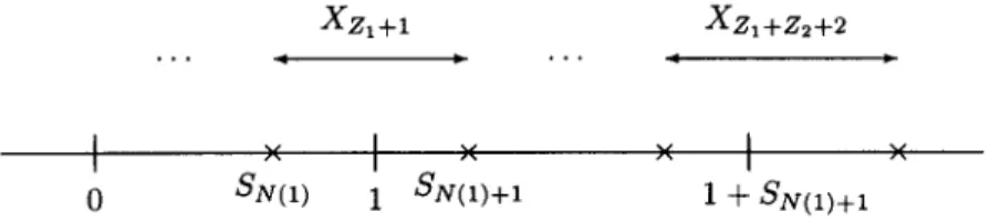
Consider two consecutive sequences of the generation of Poisson random variables, Z1 and Z2. By the m e t h o d in 2.1, we require Z1 + 1 independent uniform random numbers to generate Poisson r a n d o m variable Z1 and another Z2 + 1 independent uniform random numbers to generate Poisson random variable Z2. Indexing these two sequences of uniform random numbers together, we need Z1 + Z2 + 2 independent uniform random variables to generate Poisson random variables Z1 and Z2 (see Figure 2).
XZ1 +1 Xz1 +z2+2
• . • q D • . . ~
I × I >< × I ×
0 SN(t) 1 •N(1)+I 1 -~ SN(1)+I
Figure 2. Two consecutive sequences of the generation of Poisson random variables Z1 and Z2.
XzI+I is the interarrival which crosses the time 1. Can we use it as an exponential random
number to generate Z2? The answer is NO because Z1, Xzl+t is not independent by
36 T.-C. Lu et al.
Furthermore, the interarrival time X z , +i is selected by the inspection of time 1. The distribution of X z , + l is not exponential anymore. This is an inspection paradox in renewal theory [6]. However, we can still use XZl+l tactically to generate the next Poisson random number as discussed below. We need the following definition before the discussion.
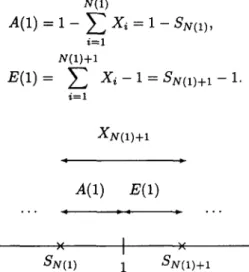
DEFINITION 2.
A(1): the time from the N(1) th arrival to time 1; E(1): the time between 1 and the (N(1) + 1) th arrival.
In Figure 3, X z l + l = XNO)+I = A(1) + E(1) where g(1) A ( 1 ) = 1 - x , = 1 - S N ( 1 ) , i = 1 N(1)-{-1 i = 1 XN(1)+I A(1) E(1) )(
I
)( SN(1) 1 SN(1)+IFigure 3. The interarrival time crosses the time 1.
Since X~ is the interarrival time with exponential distribution, N ( t ) , t >_ 0 is a Poisson process. From the memoryless property of Poisson process, the time from t = 1 to the next arrival is exponentially distributed and is independent of all that has previously occurred, so A(1) and E(1) are independent, and E(1) is an exponential random variable with mean 1/#. Since E(1) is an exponential random variable with mean l / i t , we can use E(1) to generate Z2 (see Figure 4).
A(1) E(1) A(2) E(2)
i x J x x i x
0 SN(1) 1 SN(1)-{- 1 •N(2) 2 SN(2) +1 Figure 4. The memorylees property in interarrivM time.
In turn, we can prove E ( n ) is an exponential random variable with mean 1/it, and it can be used to generate Poisson random variable Zn+l, so we have the following theorem.
THEOREM 2. Let
E ( n ) = SN(n)+I -- n, n = 1 , 2 . . . , A ( n ) = n - SN(n), n = 1 , 2 . . . ; then
i. E ( n ) is exponential distribution with mean 1~it; 2. A ( n ) and E ( n ) are independent.
Parallel Poisson Generator 37
From T h e o r e m 2, we can improve the sequential algorithm in Section 2.1 to get Z 1 , . . . , Zm in a sequence of uniform r a n d o m variables R1, R 2 , . . . , Rj without restart, where j = min{k I
R1 * R2 * . . . * Rk <_ e-mU}. T h e resulting algorithm is presented below.
PROGRAM 2.
P R O C E D U R E Sequential_Poisson_without_restart( rn, # )
/ * Procedure Uni]orm(R) generates a r a n d o m n u m b e r R-U(O, 1) * /
R R := 1; Z := 0; T := e-U; count := 0; W H I L E (count < m ) DO W H I L E ( R R > T ) DO
Uniform(R);
R R := R R * R; Z : = Z + I ; E N D W H I L E W H I L E ( R R <_ T ) DO O U T P U T ( Z - 1 ); R R := R R / T ;Z := 1 ; / * From T h e o r e m 2, R R / T is a new r a n d o m variable */
count := count + 1;
E N D W H I L E E N D W H I L E E N D P R O C E D U R E
B y T h e o r e m 2, E ( n ) is an exponential distribution with mean 1/#, and so N ( n ) - N ( n - 1) is the n u m b e r of the exponential arrivals between time n - 1 and n (see Figure 5). Thus,
Zn = N ( n ) - N ( n - 1) is a Poisson distribution r a n d o m variable with m e a n # (N(0) = 0 by
definition), so the following corollary is obtained.
COROLLARY 2. L e t Zn be the n th Poisson random variable we generated; then Zn = N ( n ) -
N ( n - 1), n = 1 , . . . , m .
A ( n - 1 ) E ( n - 1) A ( n ) E ( n )
x I x x I x
N ( n - 1) th arrival N ( n ) th arrival
Figure 5. E(n) is an exponential distribution random variable with mean 1/~. k
We therefore can c o m p u t e Sk = ~ i = l - ( 1 / # ) l n R ~ , k = 1 , . . . j. If i - 1 < Sk <_ i, the
k th arrival is in the time interval (i - 1,
i]. Counting
the arrivals in each interval (i - 1, i], we can get the Poisson r a n d o m variable Z~. We develop the following algorithm using this m e t h o d to get m Poisson r a n d o m variables. And the paxallelization of the algorithm is discussed in the next section.PROGRAM 3.
P R O C E D U R E Pseudo_code_of_Poisson( m, ~u )
S t e p 1: G e n e r a t e "sufficient" uniform r a n d o m n u m b e r s such t h a t m Poisson numbers can be generated by using them. Assume t h e m to be R1 . . . . , Rj.
38 T.-C. Lu et al. k
S t e p 3: Compute Sk = ~-~i=1Xi for k = 1 , . . . ,j.
S t e p 4: Partition {Sk I k -- 1 , . . . , j } to U~=IT~ where Ti -- {Sk I i - 1 < Sk _< i}, the cardinality of Ti is the number of arrivals in the time segment (i - 1, i].
S t e p 5: Count the cardinality of Ti for i -- 1 , . . . , m, and o u t p u t them. END P R O C E D U R E
3 . A P A R A L L E L P O I S S O N G E N E R A T O R
We develop a parallelization for the algorithm in Program 3 on E R E W P R A M model. We are concerned with the following key problems in parallelization:
1. How to generate "sufficient" uniform random numbers in parallel (Step 1). k
2. How to compute Sk -~ ~i=1 X i for k -- 1 , . . . , j concurrently (Step 3). 3. How to compute the cardinality of Ti for i -- 1 , . . . , m effectively (Step 5). These three problems will be dealt with in the following sections one by one.
3.1. A P a r a l l e l U n i f o r m R a n d o m N u m b e r G e n e r a t o r
In a parallel computing model, a parallel uniform random number generator ( P U R N G for short) is to produce a sequence of random real numbers in [0, 1) on each processor. On an E R E W PRAM, a common memory can be accessed by each processor. We can implement the G F S R algorithm presented in [7] on an E R E W PRAM directly as follows.
T h e G F S R algorithm consists of two phases: the initialization phase and the random generating phase. In the first phase, a table is constructed in the common memory. In the second phase, each processor reads two words from the table, and then makes an XOR operation to obtain a uniform random number.
When the number of processors is a power of two, the G F S R algorithm can be implemented without the common memory [4]. It can avoid communication costs.
T h e total number of "sufficient" uniform random numbers has no upper bound. We generate and process these random numbers iteratively. The algorithm generates n uniform random num- bers in each iteration with each processor sharing n i p numbers and stops when Skn > m after
t h e k th iteration. For the ith iteration, X ( i - 1 ) n + l , . . . , Xi×n are computed and the prefix compu- tation is applied to obtain S(i-1)n+l, • •., Si×n and the cardinalities of Ti,'s (the cardinality of Ti, is the number of arrivals in the time segment (i' - 1, i')). In Sections 3.2 and 3.3, we describe how to compute them in parallel.
3.2. T h e P a r a l l e l P r e f i x A l g o r i t h m
k
We use the parallel prefix computation to compute Sk -- ~ = 1 Xi for k -- 1 . . . . , n concurrently. Given X1 . . . . , Xn, the prefix computation problem is to evaluate all products X1 ®)(2 ®.- • @ X~, for i -- 1 . . . . , n, with an associative operation ®. There have been a few parallel algorithms to solve this problem under different architectures. Kruskai et al. [8] developed a parallel prefix algorithm on an E R E W PRAM model with time complexity O ( n / p + logp) where p is the number of processors. Dekel et al. [9] and Chen et al. [10] designed O(log n) algorithms on an n-leaf complete binary tree model. Moreover, E~ecio~lu et al. [11] presented an O ( n / p + logp) algorithm in hypercube, and Chen et al. [12] designed an O(nW9) algorithm on two-dimensional mesh-connected computers with multiple broadcasting (2-MCCMB's).
The prefix algorithm in [8] is adopted to construct our Poisson number generator. Accordingly, the computation model and the syntax style to specify the generator are similar to [8]. The following syntax appears frequently in our algorithm:
Parallel Poisson Generator 39
F O R A L L i E A DO IN PARALLEL BODY.
This syntax indicates that the B O D Y is executed once for each processor i in the index set A. 3.3. C o u n t i n g t h e C a r d i n a l i t i e s o f Ties in P a r a l l e l
To count the total number of elements in each segment Ti, we define an operator @ as follows.
DEFINITION 3.
( a , b + d ) i r a = c , (a, b) @ (c, d) = (c, d) if a < c,
(a,b) ira > c.
It is easy to check whether @ is associative. By the definition of Ti, we have s -- i for s in (i - 1, i]. We define an array T T with TT[k] -- Sk for k -- 1 , . . . , n ; then the frequency that
i appears in array T T is the cardinality of Ti. Since T T is nondecreasing, a _< c is always true.
Define W[i] to be (TT[i], 1), for i -- 1 , . . . , n, and call the procedure Parallel_Prefix_G to compute
all prefixes of array W and store them in array U. The second coordinate of the last element in each corresponding segment of array U represents the total number of elements in this segment. The above is summarized in the following theorem.
THEOREM 3. If T T is nondecreasing and TT[k] ~ TT[k + 1], i.e., TT[k] is the last dement of the segment
TTT[k],
then(TT[1], 1) @ (TT[2], 1) @ . . . (9 (TT[k], 1) = (TT[k], the cardinality of TTT[k]). EXAMPLE 1. Assume {Sk[ k -- 1 , . . . , 10} = {0.1, 0.3, 0.6, 0.8, 1.2, 1.3, 2.5, 2.8, 2.9, 3.1}; then T1 -- {0.1,0.3, 0.6, 0.8}, T2 = {1.2, 1.3}, T3 = {2.5,2.8,2.9}, and T4 = {3.1}. Therefore, T T [ 1 . . . 1 0 ] = [1,1,1,1,2,2,3,3,3,4], and W [ 1 . . . 10] = [(1, 1), (1, 1), (1, 1), (1, 1), (2, 1), (2, 1), (3, 1), (3, 1), (3, 1), (4, 1)]. After prefix computation,
U [ 1 . . . 10] -- [(1, 1), (1, 2), (1, 3), (1,4), (2, 1), (2, 2), (3, 1), (3, 2), (3, 3), (4, 1)].
The second coordinates of U[4], U[6], U[9], and U[10] are 4, 2, 3, and 1, respectively, which are the cardinalities of T1, T2, T3, and T4.
40 T.-C. Lu et al.
3.4. T h e Parallel Algorithm
The parallel algorithm developed from Sections 3.1-3.3 is shown in Program 4. First, each processor generates nip uniform random numbers, stores them in array R, and computes array X by assigning - ( 1 / # ) l n R [ i ] to X[i]. Next, accumulate the Sin] value (variable oldS) in the last iteration, and call the procedure Parallel_Prefix_+ to compute prefix sums (will be stored in array S) in array X based on addition operation.
We then compute array T T and W, which were discussed in Section 3.3. Before the procedure Parallel_Prefix_@ is called, the U value is accumulated in the last iteration (variable oldU). In the next step, we will look for the last element of each segment. This can be done by checking whether the T T value of an element differs from its next element. We then use array V to denote these last elements, which are finally output, and save the residual values in this iteration. PROGRAM 4. A parallel Poisson number generator.
PROCEDURE Parallel_Poisson(m, #)
/* The procedure produces m Poisson numbers with mean # */
/* Procedure Init_Uniform 0 constructs the initial table that is used in GFSR algorithm. Proce- dure Uniform(R) generates a random number R " U(0, 1); Procedure Parallel_Prefix_®(n, p, X, S) compute S[k] = ~-~k=l X[i] for k = 1 , . . . , n under operator ® on p processors EREW PRAM. */ /* Initialization */
Init_Uniform0;
oldS := 0; a := n/p;
/* Begin iteration */ WHILE (oldS <_ ra) DO /* Step 1 and Step 2 */
FORALL i ~ ( 1 , . . . ,p} DO IN PARALLEL FOR j := 1 TO a DO Uniform(R[/]); X[(i - 1) . a + j] := - l n R [ i ] / ~ END FOR END FORALL
/* Accumulate the S value in the last iteration */ X[I] := X[1] + oldS;
/* Step 3 */
Parallel_Prefix_+ (n, p, X, S);
/* Output or accumulate the U value in the last iteration */ FORALL i E {1,... ,p} DO IN PARALLEL FOR j := 1 TO a DO T T [ ( i - 1 ) * a + j ] := S [ ( i - 1) * a + j ] ; W[(i - 1) * a + j] := (TT[(i - 1) * a + j], 1) END FOR END FORALL
IF (oldS ~ 0 and oldTT ¢ TT[1]) THEN
OUTPUT(oldU)
END IF
IF (oldS ¢ 0 and oldTT = TT[1]) THEN
W[1] := (TT[1], 1+ second_coordinate of oldU)
END IF /* Step 5 */
Parallel_Prefix_@ (n, p, W, U);
Parallel Poisson Generator 41
F O R j := 1 T O a DO
V [ ( i - 1 ) . a + j] : - - 0
E N D F O R E N D F O R A L L
/* Find the last element of each segment * / F O R A L L i E { 1 , . . . ,p} DO IN P A R A L L E L F O R j : = I T O a - 1 DO I F (TT[(i - 1 ) , a + j] ~ T T [ ( i - 1) * a + j + 1]) T H E N y [ ( i - 1 ) , a + j ] := 1 E N D IF E N D F O R E N D F O R A L L F O R A L L i e { 1 , . . . , p - 1} DO IN P A R A L L E L IF (TT[i * a ] ¢ TT[i * a + 1]) T H E N Vii • a] := 1 E N D I F E N D F O R A L L /* O u t p u t U */ F O R j := 1 T O a DO F O R A L L i • { 1 , . . . ,p} DO IN P A R A L L E L IF (V[(j - 1) * p + i] = 1 and T T [ ( j - 1) * p + i] _< m) T H E N O U T P U T ( U [ ( j - 1 ) , p ÷ i]) E N D IF E N D F O R A L L E N D F O R
/* Save values in this iteration */
oldS := X[n]; o l d T T := TT[n]; oldU := U[n]
E N D W H I L E E N D P R O C E D U R E
T h e time complexity of the algorithm is not deterministic. T h e algorithm uses O(1) preprocess- ing time if the initial time of the parallel uniform r a n d o m number generator is not considered. In average, to generate m Poisson numbers needs m # uniform r a n d o m numbers and Fm~/nl itera-
tions. Since each iteration takes O ( n / p + logp) time, the average time complexity of the parallel
Poisson algorithm is O ( F m # / n 1 ( n / p + logp)). It is not time-effective when n > m # because it
is worse t h a n the case where n = m # . If n is near m # , the time complexity is O ( m # / p ÷ logp).
This algorithm achieves linear speedup for small p (the sequential algorithm takes O ( m # ) time
in average), and takes O ( l o g m # ) time where p = O(m#). The space complexity is clearly O(n).
EXAMPLE 2. Given m ---- 6, # -- 10/3, n = 12. T h e following table shows the process of this algorithm: R X S T T U V 0.010559 1.365222 1.365222 2 (2, 1) 1 0.003967 1.658893 3.024115 4 (4, 1) 0 0.335154 0.327949 3.352064 4 (4, 2) 1 0.033265 1.020973 4.373037 5 (5, 1) 0 0.355724 0.310080 4.683117 5 (5, 2) 1 0.217200 0.458081 5.141198 6 (6, 1) 0 0.536973 0.186542 5.327740 6 (6, 2) 0 OVql~ 31:3-D
42 T.-C. Lu et al.
The output sequence is (2, 1), (4, 2), (5, 2), (6, 5). It represents the Poisson number sequence: 0, 1,0,2,2,5.
4. C O N C L U S I O N
In this paper, we combine the memoryless property of Poisson process with the prefix compu- tation to parallelize a simple sequential Poisson number generator. It seems to be hard to develop parallel generators without the memoryless property.
The parallel algorithm developed in this paper is based on EREW PRAM, and we can easily modify the generator on popular architectures such as the binary tree, hypercube and 2-MCCMB.
R E F E R E N C E S
1. A. De Matteis and S. Pagnutti, Parallelization of random number generators and long-range correlations, Numer. Math. 53, 595-608 (1988).
2. A. De Matteis and S. Pagnutti, A class of parallel random number generators, Parall. Comput. 13 (2), 193-198 (1990).
3. I. De, Uniform random number generators for parallel computers, ParaU. Comput. 15 (1-3), 155-164 (1990). 4. S. Aluru, G.M. Prabhu and J. Gustafson, A random number generator for parallel computers, Parall. Comput.
18 (8), 839-847 (1992).
5. D.E. Knuth, The Art of Computer Programming, Vol. 2: Seminumerical Algorithms, 2 ad edition, Addi- son-Wesley, New York, (1981).
6. S.M. Ross, Introduction to Probability Models, Academic Press, London, (1985).
7. T.G. Lewis and W.H. Payne, Generalized feedback shift register pseudorandom number algorithm, J. A C M 20 (3), 456-468 (1973).
8. C.P. Kruskal, L. Rudolph and M. Snir, The power of parallel prefix, IEEE Tran. Comput. C - 3 4 (10), 965-968 (1985).
9. E. Dekel and S. Sahni, Binary trees and parallel scheduling algorithms, IEEE Tran. Comput. C - 3 2 (3), 307-315 (1983).
10. R.J. Chen and Y.S. Hou, Non-associative parallel prefix computation, Inform. Process. Lett. 44 (2), 91-94 !.1992).
11. O. E~ecio~lu, O.K. Koq and A.J. Lanb, A recursive doubling algorithm for solution of tridiagonal systems on hypercube multiprocessors, J. Comput. Applic. Math. 27 (1/2), 95-108 (1989).
12. Y.C. Chen, W.T. Chen, G.H. Chen and J.P. Sheu, Designing efficient parallel algorithms on mesh-connected computers with multiple broadcasting, IEEE Tran. Parall. Distrib. Sys. 1 (2), 241-246 (1990).