Moving Object Detection and Mosaic Construction by Image Stitching

全文

(1)Moving Object Detection and Mosaic Construction by Image Stitching Jun-Wei Hsieh Department of Electrical Engineering YuanZe University, Taoyuan, Taiwan. Tel:886-3-463-8800 Ext. 430 Fax:886-3-463-9355 shieh@saturn.yzu.edu.tw Abstract This paper proposes a novel edge-based stitching method to detect moving objects and construct mosaics from images. The method is a coarse-to-fine scheme which first estimates a good initialization of camera parameters with two complementary methods and then refines the solution through an optimization process. The two complementary methods are the edge alignment and correspondence-based approaches, respectively. Since these two methods are complementary to each other, the des ired initial estimate can be obtained more robustly. After that, a Monte-Carlo style method is then proposed for integrating these two methods together. Then, an optimization process is applied to refine the above initial parameters. Since the found initialization is very close to the exact solution and only errors on feature positions are considered for minimization, the optimization process can be very quickly achieved. Experimental results are provided to verify the superiority of the proposed method. Keywords: Image registration, image-based rendering, mosaics, moving object detection, and video retrieval.. 1. Introduction Image stitching is the process of recovering the existing camera motions between images and then compositing them together. This technique has been successfully applied to many different applications like video compression [1], video indexing [2]-[3], object tracking [9], or creation of virtual environments [5]-[8], [12]. For example, Shum and Szeliski [7]-[8] proposed methods to stitch a set of images together to form a panorama. In addition, Irani and Anandan [2] used this technique to represent and index different video contents. Moreover, Jin et al. [9] used this technique to compensate unwanted camera motions for extracting desired objects from video sequences. For most methods in this field, an affine camera. model is used to approximate the possible motions between two consecutive frames. Then, the parameters of this model can be recovered from pair of images by two common methods, i.e., the correlation-based approach and the optimization-based one. For the first approach, the measure “correlation” can be calculated in frequency domain or spatial domain. For example, Kuglin and Hines [4] presented a phase-correlation method to estimate the displacement between two adjacent images in frequency domain. For the approaches in spatial domain, Sawhney and Ayer [1] proposed a feature matching approach to estimate the dominant and multiple camera motions. In addition, Zoghlami et al. [11] proposed a corner-based approach to build a set of correspondences for computing the transformation parameters from pair of images. However, the establishment of good correspondences is a challenging work when images have nonlinear intensity changes [17]. In order to avoid this problem, some researchers [6], [13] treated the stitching problem as a global optimization problem. For example, Szeliski [6] proposed a nonlinear minimization algorithm for automatically registering images by minimizing the discrepancy in intensities between images. In addition, Davis [13] proposed an optimization scheme to obtain a least-square solution by globally optimizing all pair-wise registrations. In comparison with the correlation-based method, the global optimization approach performs more robustly but will be trapped on a local minimum if the starting point is not properly initialized. In this paper, we present an edge-based stitching technique to detect moving objects and construct mosaics from consecutive images. In general, the transformations between consecutive images can be described by a planar perspective motion model. Since the transformation is non-linear, the paper uses a coarse-to-fine approach to robustly and accurately recover the desired model parameters. Firstly, at the coarse stage, two.

(2) complementary methods, i.e., the edge alignment and the correspondence-based approaches, are proposed to get respective initial estimates from images. Then, at the fine stage, the found initial estimate can be further refined through an optimization process. The edge alignment method finds possible image translations by checking the consistencies of edge positions between different images. It is simple and efficient without involving any optimization process or building any correspondences. In addition, the method has better capabilities to overcome large displacements and lighting variations between images. On the other hand, the correspondence-based method obtains desired model parameters from a set of correspondences by using a new feature extraction and a new correspondence building method. Especially, when building correspondences, a new measure is defined to measure the goodness of each match such that all false correspondences between features can be eliminated as well as possible. Compared with the edge alignment method, the correspondence-based approach can solve more general camera motion model but fails to work when images have large lighting changes. Therefore, due to the complementary property of the two methods, we can obtain the desired initial estimate more robustly. After that, a Monte-Carlo style method with gird partition is then proposed to integrate these methods together. The grid partition scheme can much enhance the accuracy of each try for deriving the correct parameters. Then, the found parameters are further refined through an optimization process. Sine the minimization is only applied to the positions of matching pairs, the optimization process can be performed very efficiently. From experimental results, the proposed method indeed achieves great improvements in terms of stitching accuracy, robustness, and stability. The rest of the paper is organized as follows. In the next section, we will present an affine model to appro ximate the motions of a video camera. Then, details of the proposed method for recovering the parameters of this model are described in Section III. Section IV reports the experimental results. Finally, conclusions will be presented in Section V.. 2. Camera Motion Model Assume that input images are captured by a video camera. Then, the relationship between two adjacent images can be described by an affine camera model:. m0 x + m1 y + m3 m x + m4 y + m5 and y ' = 3 ,(1) m6 x + m7 y + 1 m6 x + m7 y + 1 where (x, y) and ( x ', y ') are a pair of pixels in the x' =. two adjacent images I 0 and I1 , and M = (m0 , m1 ,..., m7 ) the motion parameters. The M can be obtained by minimizing the error function E(M) as follows: E ( M ) = ∑ [ I 1 (xi' , yi' ) −I 0 (x i , yi )]2 = ∑ ei2 , (2) i. i. where ei = I1 ( x i' , yi' ) − I 0 (x i ,y i ) . Then, Szeliski[7] gave the solution M with the iterative form: M T ← M T + ∆M T , (3) T where ∆M = ( A + λ I )− 1 B , A = [ akn ] , B = [bk ] ,. akn = ∑ ∂mik ∂e. i. ∂ei ∂m n. , bk = ∑ ei. ∂ei ∂m k. , and λ. is a. i. coefficient obtained by the Levenber-Marquardt method [18]. The method works well if the initial value to the correct M is close enough. However, it suffers from low convergence and gets trapped in local minimum if the initialization is not proper, especially when images have large displacements. It is noticed that Eq.(3) tries to find desired solutions by minimizing intensity errors of all pixels between images. When the number of iterations increases, the calculation of intensity errors will become very time-consuming. Therefore, in what follows, we will propose a fast edge-based algorithm for tacking all the above problems.. 3. Fast Algorithm for Mosaic Construction and Object Detection In this paper, a coarse-to-fine approach is proposed to guide the optimization process. First, an edge-based approach is proposed to find a good initial estimate and then the initial result is refined through an optimization process. The initial estimate is got from two complementary methods, i.e., the edge alignment and the correspondencebased approaches. Since the two methods are complementary to each other, the robustness of the whole process of parameter estimation can be much enhanced. After that, a Monte Carlo style method is then used to integrate the above solutions together. For accuracy consideration, the found parameters can be further refined with an optimization process, which minimizes errors only on the coordinates of feature points. Sine the number of feature points is much smaller than the whole image, the optimization process can be performed extremely efficiently. The overall flowchart of the proposed approach is described in Fig. 1. In what follows, details of each proposed algorithm are described..

(3) 3.1 Translation Estimation Using Edge Alignment As described in Fig. 1, for the purpose of robustness, we propose two strategies to find different initializations fed into an optimization process for deriving the correct model parameters. In this section, the edge alignment method is first proposed to estimate desired model translations from images. Let g x ( p ) be the gradient of a pixel p in the x direction of an image I, i.e., g x ( p(i , j )) =| I ( p (i + 1, j )) − I ( p(i − 1, j ))| , where I ( p) is the intensity of p. In addition, let. S g (i ) denote the sum of g x ( p ) obtained by accumulating g x ( p ) along pixels in the ith column, i.e., 1 S g (i ) = ∑ | I ( p(i + 1, j )) − I ( p (i − 1, j ))| , H j where H is the height of I. If S g ( i ) is larger than a threshold, i.e., 15, the ith column is considered to have a vertical edge. After checking all pixels of input images column by column, a set of positions of vertical edges can be found. Assume I a and I b are two images prepared to be stitched and shown in Fig. 2 (a) and (b), respectively. Through the above vertical edge detector, the positions of vertical edges in I a and I b can be obtained as Pav = (100, 115, 180, 200, v b. 310, 325, 360, 390, 470) and P = (20, 35, 100, 120, 230, 245, 280, 310, 390), respectively. If the images I a and I b come from the same static scene, there should exist an offset d x such that Pav (i ) = Pbv ( j ) + d x and the corresponding relation between i and j is one-to-one. Then, the offset d x is the desired translation solution between I a and I b in the x direction, i.e., d x = 80. Based on this idea, in what follows, a novel method will be proposed to estimate desired translation parameters from images without building any correspondences or involving any optimization processes. Before describing the proposed method, we shall know in practice due to noise, some edges will be lost or undetected. The lost or undetected edges will lead to that the relations between Pav. and Pbv are no longer one-to-one. For this problem, this paper defines a distance function dv (i , k ) to measure the distance of a position. Pav (i ) to the translation solution k as. dv (i , k ) = minv | Pav (i ) − k − Pbv ( j ) | , 1≤ j ≤ N b. (4). where N bv is the number of elements in Pbv . Let Td denote a threshold and set to be 4. Given a number k, we want to determine the number N vp of elements in Pav whose dv (i , k ) is less than Td . In addition, we denote the average value of. dv (i, k ) for these N vp elements as E kv , which can be used as an index to measure the goodness of k to see whether it is a suitable translation solution. If Ekv is smaller enough and N vp is larger enough, the position k will be a good horizontal translation. More precisely, if Ekv ≤ Te and N vp ≥ T p , the k is collected as an element of the set S x of possible horizontal translations, where the two thresholds T p and Te are set to be 5 and 2,. respectively. Let Wb denote the width of the input image I b . Through examining different k for all | k |< Wb , the set S x can be obtained. On the other hand, let Pah and Pbh denote as the sets of horizontal edge positions in I a and I b , respectively. With Pah and Pbh , we can define a distance function d h as follows: dh (i , k ) = minh | Pah (i) − k − Pbh ( j ) | , 1≤ j ≤ N b. (5). where N bh is the number of elements in Pbh . Let H b denote the height of the input image I b . According to dh , with the similar method to obtain S x , by examining different k for all | k |< H b , the set S y of possible vertical translations can be obtained. With S x and S y , the set. S xy. of possible translations can be. obtained as: S xy = {( x , y ) | x ∈ S x , y ∈ S y } .. The. best translation can be then determined from S xy through a correlation technique. Details of the whole algorithm are summarized as follows. Edge-based Translation Estimation Algorithm: I a and I b : two adjacent images prepared to be stitched. S1: Apply a vertical edge detector to find the sets Pav and Pbv of vertical edge positions from I a and I b , respectively..

(4) S2: Determine the set S x of possible horizontal Pav. Pbv. translations from and based on dv (i , k ) (see Eq.(4)). S3: Apply a horizontal edge detector to find the sets Pah and Pbh of horizontal edges from I a and I b , respectively. S4: Determine the set S y of possible vertical translations from Pah and Pbh based on dh (i , k ) ( see Eq.(5)). S5: Let S xy denote the set of possible translations, i.e., S xy = {( x , y ) | x ∈ S x , y ∈ S y } .. maxima of M 2 I ( x , y ) , and M 2 I ( x , y ) > a threshold; C2: | ∇I σ ( x , y) |σ =2 =. max {| ∇I σ ( x ', y ')|σ = 2 } ,. ( x' , y ' )∈N p. where N p is a the neighborhood of P(x,y) within an 13×13 window.. 3.2.2 Correspondence Establishment In the previous section, we have described how the feature points between I a ( x , y ) and I b ( x , y ) are derived. Now, we are ready to find the matching pairs between I a and I b . Let FPI a = { pi =. ( pix , piy )} and FPI b = {qi = (qxi ,qiy )} be two sets. S6: Determine the best solution (tx ,t y ) from S xy through a correlation technique.. of feature points extracted from two images I a and I b , respectively. In addition, N I a and N I b. 3.2 Motion Parameter Estimation by Feature Matching. represent the number of elements in FPI a and. As described in Fig. 1, two strategies are used to find respective initial estimates of camera parameters for further optimization process. In this section, details of the correspondence-based method are described. In Section 3.2.1, we will propose a new method to extract a set of useful feature points from images based on edges. Then, details of building correspondences between features are described in Section 3.2.2. However, due to noise, many false matches will also be generated. In Section 3.2.3, a new scheme is proposed to eliminate all impossible false matches.. 3.2.1 Feature Extraction In this section, we will use several edge operators to extract a set of useful feature points. First of all, let the gradients of an image I(x,y) at scale σ in the x and y directions be denoted as I xσ ( x , y ) = I * G ( x , y ) and I ( x , y ) = I * G ( x, y ) , where σ x. σ y. σ y. FPI b , respectively. The similarity between two feature points p and q is measured by their normalized cross-correlation denoted as C ( p, q ) .. For each point pi in FPI a , find the maximum peak of the similarity measure as its best matching point q in another image I b . Then, a pair { pi ⇔ qi } is qualified as a matching pair if two conditions are satisfied: C ( pi , qi ) = max C ( pi , qk ) and C ( pi , qi ) ≥ Tc , (6) q k ∈FPIb. where Tc = 0.75 . The first condition enforces to find a feature point qk ∈ FPI b such that the measure CI a ,I b is maximized.. As for Condition. 2, it forces the value CI a ,I b of a marching pair to be larger than a threshold (0.75 in this case).. 3.2.3 Eliminating False Matches. 2D Gaussian smoothing function Gσ ( x , y ) in the x and y directions, respectively, where σ is a standard deviation. Then, the modulus of I σx. In the previous section, through matching, a set of matching pairs has been extracted. However, if the relative geometries of features are considered, the matching results can be refined more accurately. Let MPIa , Ib = { pi ⇔ qi }i =1,2... be the set of. and I σy is defined as:. matching pairs, where pi is an element in FPI a. | ∇I σ ( x , y ) |= | I σx ( x , y) |2 + | I σy ( x , y ) |2 . Since we are interested in some specific feature points for image stitching, additional constraints have to be introduced. In what follows, two conditions adopted here for judging whether a point P(x,y) is a feature point or not are summarized as follows: C1: P(x,y) must be an edge point of the image I(x,y). This means that P(x,y) is a local. and qi another element in FPI b . Let NeI a ( pi ). Gσx and. Gσy are the first partial derivatives of a. and NeIb (qi ) be the neighbors of pi and qi within a disc of radius R, respectively. Assume that NPpi q j = {nk1 ⇔ nk2 }k =1,2.... is the set of matching pairs, where. n1k ∈ NeI a ( pi ) ,. nk2 ∈. NeIb (q j ) , and all elements of NPpi q j belong to MPI a ,Ib .. The proposed method is based on a.

(5) concept that if. { pi ⇔ qi }. and. {p. ⇔ q j } are. j. two good matches, the relation between pi and p j should be similar to the one between qi and q j . Based on this assumption, we can measure. the goodness of a matching pair according to how many matches. {n. 1 k. { pi ⇔ qi }. ⇔ nk2 } in. NPpi qi whose distance d( pi , n1k ) is similar to the. distance d( q j , nk2 ), where d ( ui , u j ) =|| ui − u j || , the Euclidean distance between two points ui and u j . Then, the measure of goodness for a match. { pi ⇔ qi }. can be defined as:. GI a Ib (i ) =. C (n1k , nk2 )r( i, k ) , 1 + dist (i , k ) {n 1k ⇔nk2 }∈NPpi qi. ∑. where dist (i , k ) = [d ( pi , n1k ) + d ( qi , nk2 ) ] / 2 , C ( n1k , nk2 ) the correlation measure between n1k and nk2 , r (i , k ) = e − µ (i ,k )/ T1 , with a threshold T1 , and u( i, k ). = | d ( pi , nk1 ) − d ( qi , nk2 ) | / dist (i , k ) . The contribution. of a pair {n1k ⇔ nk2 } in NPpi qi monotonically decreases based on the value of dist(i, k). After calculating the goodness of each pair { pi ⇔ qi } in MPIa ,I b , we can obtain their relative goodness GIa I b (i ). for further eliminating false. matches. Assume G is the average value of GIa I b (i ) for all matching pairs. If the value of GIa I b (i ) is less than 0.75 G , the matching pair. { pi ⇔ qi }. is eliminated.. 3.3 Motion Parameter Estimation Using Monte Carlo Method In this section, a Monte-Carlo -style method is proposed for integrating these methods together for further optimization process. The spirit of the Monte Carlo method is to use many tries to find (or hit) the wanted correct solution. Assume each try can generate a solution and the probability to find a correct solution for each try is r. After k tries, the probability of continuous failure to find a correct solution is s = (1 − r)k . Clearly, even though r is very small, after hundreds or thousands of tries, s will tend very closely to zero. In other words, if we define a try as a random selection of four matching pairs, each try will generate a solution. Then, it is expected that a correct solution M will be obtained after hundreds or thousands of tries. As we knew, for each try, four matching pairs. will be selected to obtain a possible solution. If MPr has N r elements and N c ones are correct, the probability to select four correct pairs for each N c ( N c − 1)( N c − 2)( Nc − 3) try will be . In what N r ( N r − 1)( N r − 2)( N r − 3) follows, a method is proposed to improve the probability for each try to find a correct solution by separating images into grids. Assume all the correct and false matching pairs distribute very randomly. Then, if the input images are segmented into several grids, in each grid the probability to select a correct matching pair is still N c / N r . Therefore, we can select four different girds first and then get one matching pair from each grid. With this method, the probability to select four correct matching pairs will become N c ( N c − 1)( N c − 2)( Nc − 3) N c4 / N r4 . Clearly, < N r ( N r − 1)( N r − 2)( N r − 3) N c4 / N r4 if N c < N r . Thus, the suggested method can better enhance the hit rate of finding four correct matching pairs to derive desired parameters. On the other hand, since the Monte Carlo method uses lots of tries to find final desired solutions, we should propose a verification process to determine which try is the best. Assume M i = ( m0i , m1i ,..., m7i ) is the solution got from the ith try. The verification process can be achieved by comparing how many matching pairs in MPr. { p ↔ q} be a. M i . Let. are consistent to. matching pair and the consistent error e( p , q , M i ) of this pair to M i be: m p +m p + m m p + m p + m .(7) e ( p , q , M ) = (q − ) + (q − ) i. x. i 0. x. i 1. y. i 2. m6i p x + mi7 p y + 1. 2. y. i 3. x. i 4. y. i 5 2. mi6 p x + m7i p y + 1. For each matching pair { pk ↔ qk } in MPr , if e( pk , qk , M i ) < Te , the pair { pk ↔ qk } is said to. be consistent to M i , where Te is a threshold set to 6 for the consistency check. Based on Eq.(7), a counter c( M i ) is used to record how many matching pairs in MPr which are consistent to M i . After several tries, the best solution M can be obtained as follows: M = argmax c( M i ) . (8) i M. When initialization (i=0), M 0 is got from the edge alignment approach (see Section 3.1).. 3.4 Parameter Refinement through Optimization With the Monte Carlo method, the best estimate.

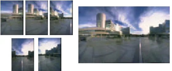
(6) M can be found from MPr .. However, if an M optimization process is applied, can be further refined. In Section 3.2, two sets of feature points, i.e., FPI a and FPIb , have been extracted from the images I a and I b , respectively. For each point pi in FPI a and q j in FPI b , according to Eq.(7) and. M ,. e( pi , qj ,M ) < Te , we denote. if. { pi ⇔ q j } as a new match.. Then, after checking. all elements in FPI a and FPI b , a new set MPM of matching pairs can be obtained: MPM = {p k ⇔ qk , k = 1,2,..., N M } , where e( pk , qk ,M ) < Te , pk ∈ FPI a , and qk ∈ FPI b . Then, we can define an error function as: NM. Φ( M ) = ∑ e( pk , qk ,M ) ,. (9). k =1. where { pk ⇔ qk } is an element in MPM . By calculating the gradient and Hessian matrix of Φ , M can be updated with the iterative form: M tT+1 = M tT + ( A + λ )−1 B , (10) NM. where. [ A]ij = ∑ ∂∂meki k =1. ∂ek ∂m j. NM. , [ B]i = ∑ ek k =1. ∂ek ∂m i. , t is the. iteration number, and λ is a coefficient obtained by the Levenber-Marquardt method [18]. The above minimization process quickly converges since only the coordinates of feature positions are considered into minimization and the initial estimate of M is very close to the final solution.. 4. Experimental Results In order to analyze the performance of the proposed method, a series of real images were adopted as test images. Fig. 3 shows the result for mosaic construction when a series of panoramic images are used. In this case, before stitching, all the images are projected into a cylindrical map [5]. Then, only the translation parameters need to be estimated. Fig. 4 shows the case when images have larger intensity differences. (a) and (b) are the original images and (c) is the stitching result. The large lighting changes will lead to the instability of feature matching in the traditional matching techniques like block matching or phase correlation techniques. However, in this paper, the proposed edge alignment algorithm tries to find all possible translations by checking the consistence of edge positions instead of comparing the intensity similarity of images. Therefore, even though images have larger lighting changes, the proposed method still works well to find all desired camera parameters for stitching. Fig. 5. shows the case when images have some moving objects. The moving object will disturb the work of image stitching. However, the proposed method still successfully stitches them together. Fig. 6 shows the result when images have some rotation and skewing effects. In this case, the proposed Monte Carlo method still works well to find the correct camera parameters. The proposed method also can be used in camera compensation for extracting moving objects from video sequence. Fig. 7 shows two frames got from a movie. In order to detect the moving object, a static background should be constructed. With the proposed method, the camera motion between Fig. 7(a) and Fig. 7(b) can be well found and compensated. Fig. 7(c) is the mosaic of Fig. 7(a) and (b). Then, the moving object can be detected by image differencing like Fig. 7(d). The detection result is very useful for various applications like intelligent transportation system, video indexing, video surveillance, and etc. Fig. 8 is another case when a moving car appears in the video sequence. From the experimental results, it is obvious that the proposed method is indeed an efficient, robust, and accurate method for image stitching.. 5. Conclusions In this paper, we have proposed an edge-based method for stitching series of images from a video camera. In this approach, for robustness consideration, the initial estimate is estimated from two different schemes, i.e., the edge alignment approach and the correspondence-based one. Since the two methods are complementary to each other, much robustness can be gained during the parameter estimation process. To integrate these two methods together, a Monte-Carlo style method is proposed to find the best motion parameters. Then, the solution is refined through an optimization process. The contributions of this paper can be summarized as follows: (a) This paper proposed an edge alignment scheme for estimating translation parameters using edges. The method has better capabilities to overcome the problems of large displacements and lighting changes between images. (b) A new feature extraction scheme was proposed to extract a set of useful features. (c) When building correspondences, a new scheme was proposed to eliminate many false matches by judging the goodness of a matching pair. Through the judgment, a set of desired correspondences can be obtained more reliably..

(7) (d) A grid partition scheme was proposed to enhance the hit rate of obtaining four correct matching pairs. Then, the correct parameters can be found with less tries. (e) An efficient optimization process was proposed for refining the estimated parameters more accurately. Since only the errors on feature positions are considered, the minimization process can be performed extremely efficiently. Experimental results have shown our method is superior in terms of stitching accuracy, robustness, and stability.. Acknowledges This work was supported in part by National Science Council of Taiwan under Grant NSC91-2213-E-150-019, Taiwan.. References [1] H. Sawhney and S. Ayer, “Compact representation of video through dominant and multiple motion estimation, ” IEEE trans. Pattern Anal. Machine Intell., vol. 18, 814-830, Aug. 1997. [2] M. Irani and P. Anandan, “Video indexing based on mosaic representation,” Proc. IEEE, vol.86, pp. 905-921, May, 1998. [3] M. Bonnet, “Mosaic representation for video shot description,” Proc. MPEG-7 Evaluation Ad Hoc Meeting, pp. 636, Feb. 1999. [4] C. Kuglin and D. Hines, “The Phase Correlation Image Alignment Method,” Proc. of the IEEE Int. Con. on Cybernetics and Society, pp.163-165, 1975. [5] S. Chen, “Quicktime VR-an image-based approach to virtual environment navigation,” Proc. SIGGRAPH ’95, pp.29-38, 1995. [6] R. Szeliski, “Video Mosaics for Virtual Environments,” IEEE Computer Graph and Application, vol. 16, pp. 22-30, March 1996. [7] H. Y. Shum and R. Szeliski, “Systems and Experiment Paper: Construction of Panoramic Image Mosaics with Global and Local Alignment,”International Journal of Computer Vision, vol. 36, no. 2, pp. 101-130, 2000. [8] R. Szeliski and H. Y. Shum, “Creating full view panoramic image moaics and environment maps,” Proc. Computer Graphics Annu. Conf. Series, pp. 251-259, 1997. [9] J. S. Jin, Z. Zhu and G. Xu, “A stable vision system for moving vehicles”, IEEE Trans. on Intelligent Transportation Systems, vol. 1, No. 1, pp.32-39, 2000. [10] H. Nicolas, “New methods for dynamic mosaicking,” IEEE trans. Image Processing, vol. 10, no. 8, pp. 1239-1251, Aug. 2001.. [11] I. Zoghlami, O. Faugera, and R. Deriche, “Using geometric corners to build a 2D mosaic from a set of images,” Proc. Conf. Computer Vision and Pattern Recognition, Puerto Rico, pp.420-425, 1997. [12] C.T. Hsu et al., “Feature-based video mosaic,” Proceedings of ICIP 2000, vol.2, pp.887-890, Vancouver, Canada, Sep. 2000. [13] J. Davis, “Mosaics of scenes with moving objects,” IEEE Proc. CVPR 1998. [14] C. Guestrin, F. Cozman, and E. Krotkov, “Fast Software Image Stabilization with Color Registration,” In Proceedings of Intelligent Robots and Systems Conference, pp.19-24, Victoria, Canada, October 1998. [15] S. B. Kang, “A survey of image-based rendering techniques,” Technical Report 97/4, Digital Equipment Corporation, Cambridge Research Lab. [16] J. W. Hsieh, H. Y. Mark Liao, K. C. Fan, M. T. Ko, and Y. P. Hung, “Image Registration Using a New Edge-based Approach, ” Computer Vision and Image Understanding, 67, 112-130, 1997. [17] M. Sonka, V. Hlavac, and R. Boyle, Image Processing, Analysis and Machine Vision, London, U. K.: Chapman & Hall, 1993. [18] W. H. Press, S. A. Teukolsky, W. T. Vetterling, and B. P. Flannery, Numerical Recipes in C: the Art of Scientific Computing, Cambridge University Press. Input Images. Translation Estimation Using Edge Alignment. Feature Extraction Using Edge Operators Correspondence Establishment. Motion Estimation with Monte Caro Approach Solution Refinement by Optimization. Camera Compensation or Mosaic Construction. Fig. 1: Flowchart of the proposed method.. (a) (b) Fig. 2 Edge results of two images..

(8) (a). Fig. 3: Stitching result of a series of panoramic images.. (b). Fig. 6: Stitching result when the camera has rotation changes.. (a). (a). (b). (b) (c) (d) Fig. 7: Mosaic construction and object detection. (c) is the mosaic result of (a) and (b). (d) is the object detection result by image differencing.. (c) Fig. 4: Stitching result of two images with larger lighting changes. (c) is the stitching result of (a) and (b). (a). (a). (b). (b) (c) (d) Fig. 8: Mosaics and object detection when images have a moving object. c) is the mosaic result of (a) and (b). (d) is the object detection result by image differencing. (c). Fig. 5: Stitching result when images have moving objects. (a) and (b) Original Images. (c) Stitching result..

(9)