https://doi.org/10.1007/s00382-018-04607-x
Object-based precipitation system bias in grey zone simulation:
the 2016 South China Sea summer monsoon onset
Chun‑Yian Su1,2 · Chien‑Ming Wu1 · Wei‑Ting Chen1 · Jen‑Her Chen2
Received: 20 July 2018 / Accepted: 26 December 2018 / Published online: 3 January 2019 © Springer-Verlag GmbH Germany, part of Springer Nature 2019
Abstract
This study aims to evaluate the precipitation bias in the grey zone simulation (~ 15 km) using the Central Weather Bureau Global Forecast System (CWBGFS). We develop a new evaluation method using the object-based precipitation system (OPS) to examine the bias associated with the degree of convection organization. The 2016 South China Sea (SCS) Summer Monsoon onset is selected to evaluate the model’s performance due to its sharp transition of large-scale circulation, which contributes to the complexity of precipitation pattern. The results based on OPS show that the observed precipitation tends to aggregate toward the central part of SCS during the post-onset period, while the precipitation in the model distributes more sparsely over the ocean. The observed precipitation intensity increases with the size of OPS especially for the extremes; however, the model underrepresents the relationship between the precipitation spectrum and the size of OPS. Moreover, the model simulates earlier diurnal peak time of precipitation over land in the organized systems than observation. The results also suggest that the convection scheme is insensitive to column moisture during the pre-onset period which seems to be one of the key factors to the excessive precipitation in the model. Using high horizontal resolution, however, does not improve the simulation of precipitation much in the model. The current study suggests that the precipitation bias related to aggregation of the convective systems should be regarded as an essential objective of model evaluation and improvement.
Keywords Object-based precipitation system · Precipitation bias · Grey zone simulation · Degree of convection organization · South China Sea summer monsoon onset
1 Introduction
Moist convection plays an essential role in the climate sys-tem through its interactions with the large-scale environ-ment. It redistributes heat, moisture, and energy vertically and globally through large-scale circulations. In a general circulation model (GCM), which usually has grid size larger than the spatial scale of moist convection, the collective effect of moist convection must be parameterized in terms of resolved-scale variables (i.e., cumulus parameterization, see Arakawa (2004) for a review). Although there has been tre-mendous progress in cumulus parameterization development
over the decades, the pace of progress is slow (Randall et al. 2003), and there are persistent problems in cumulus param-eterization (Flato et al. 2013).
Precipitation is generally regarded as overall results for convective activities and is used to evaluate model parame-terizations (Gustafson et al. 2014). Several studies have iden-tified the prominent precipitation biases in GCMs, which are partially contributed by parameterized convection. Stephens et al. (2010) suggested that the GCMs tend to precipitate too frequently and too lightly over the global ocean. Dai and Trenberth (2004) demonstrated that the GCM produces earlier diurnal peak time and reduced intensity of precipita-tion over land in the warm season. Fischer and Knutti (2016) argued that the models tend to underestimate the changes in heavy rainfall intensity under warmer climate based on observations from the two continents. Parameterized con-vection is also considered being responsible for the model’s deficiencies of simulating India summer monsoon (Willetts et al. 2017), intraseasonal variability (e.g., Madden-Julian Oscillation, Kim et al. 2011; Mapes and Bacmeiste 2012),
* Chien-Ming Wu mog@as.ntu.edu.tw
1 Department of Atmospheric Sciences, National Taiwan
University, No. 1, Sec. 4, Roosevelt Rd, 10617 Taipei, Taiwan, Republic of China
2 Central Weather Bureau, No. 64, Gongyuan Rd,
and the uncertainty in cloud feedbacks to climate change simulations (Sanderson et al. 2010). Part of the deficiencies in parameterized convection is related to the insensitivity of convective activity to environmental moisture (Derby-shire et al. 2004; Del Genio et al. 2012). Although the use of cloud-resolving models or the superparameterization (Khairoutdinov and Randall 2001) is considered as one of the solutions to improve the representation of convection in the global climate simulation, their practical application is constrained by the technical complexity and the demand for the computational cost.
As computer power increases, the grid size used by GCMs become finer, which can better represent local to regional scale processes such as land-sea breeze over com-plex coastlines, and mesoscale convective systems. Besides, the increase of horizontal resolution could increase the vari-abilities of simulated convection. Previous studies have also shown that increasing horizontal resolution of the model could improve the performance of the modeled precipitation extreme events (Kopparla et al. 2013). However, with the grid size of around 10 kilometers, the advantages of utilizing such high resolution are hindered by the ambiguity between the subgrid-scale and resolved scale. At this so-called “grey zone” scale, whether the moist convection should be param-eterized or not becomes questionable, and it contributes to the difficulties in representing the organized convection resulting from the lack of scale separation between convec-tive and large-scale processes. There are some recent efforts in addressing the gray-zone problem, for example, Liu et al. (2015, 2018), Zhang et al. (2015) and Yun et al. (2017), after the influential study of Arakawa and Wu (2013).
In nature, moist convection exhibits various forms of organization, ranging from isolated cells to mesoscale con-vective systems (Houze 2004). These convections behave quite differently for vertical momentum and moist static energy transport and their life cycles according to their degrees of organization (Grabowski et al. 1996; Moncrieff and Klinker 1997; Houze 2004; Moncrieff 2004; Liu et al.
2015, 2018). Using the global satellite rainfall estimates, Hamada et al. (2014) demonstrated the dependence of the precipitation extremes on the size of the precipitation sys-tem. However, the model simulated relationship between precipitation spectrum and the size of precipitation system regarding the degree of convection organization is seldom discussed.
This study develops a new evaluation method using the object-based precipitation system (OPS), which classi-fies the systems according to their size, to investigate how precipitation bias varies with the size of precipitation sys-tems in a grey-zone resolution weather forecast model with parameterized convection. The hindcast approach from Ma et al. (2013, 2015) is adopted, which allows diagnosing the model bias caused by fast processes, such as cumulus
parameterization. The 2016 South China Sea (SCS) summer monsoon onset is selected as the evaluation period, during which multi-scale interactions are active and convection of various size, lifetime, and structure can occur (Wang et al.
2004; Li et al. 2010). Section 2 presents the model descrip-tion, experiment design, the datasets, and object-based analysis method used in this study. The bias of spatial distri-bution, intensity spectrum, and diurnal variability of precipi-tating system size are presented in Sect. 3. The discussion and summary are presented in Sects. 4 and 5, respectively.
2 Methodology
2.1 Model description
The model used in this study is the Central Weather Bureau Global Forecast System (CWBGFS, Liou et al. 1997). The CWBGFS is a hydrostatic global spectral model with reduced Gaussian grids (Hortal and Simmons 1991) in the horizontal and sigma-pressure hybrid level in the vertical. The model system was updated as following the upgrade of High-Performance Computer (HPC) in CWB. The resolution used in this study is T853 (~ 15 km) in the horizontal and 60 layers in the vertical with 0.1 hPa at the model top. We note that this horizontal resolution is finer than the current opera-tional version (T512, ~ 25 km) while the vertical resolution remains the same. The time step used for dynamical core in this study is 30 s, which is the same as physics parameteriza-tions except that the radiation scheme is called for each hour. The CWBGFS not only helps guide CWB forecasters for issuing weather forecasts but also provides boundary condi-tions for a regional forecast model (Jeng et al. 1991) and a typhoon track model (Peng et al. 1993). The data assimila-tion system used for initializing the model is the grid point statistical interpolation based three-dimensional variational method and ensemble Kalman filter (Gao et al. 2013). The Noah 4-layer land surface model (Ek et al. 2003) is adopted as the land surface model. The cumulus parameterization, vertical diffusion, and shallow convection schemes are referred to Han and Pan (2011). The microphysics scheme is referred to Zhao and Carr (1997) which uses the Kessler-type parameterization (Kessler 1969) to produce grid-scale precipitation, and the radiation scheme is the RRTMG based on Iacono et al. (2008). The grid-scale cloudiness is diag-nosed following Xu and Randall (1996). The gravity drag parameterizations include topography (Palmer et al. 1986) and convection (Scinocca 2003). Besides orography-induced gravity waves, convection can be a possible source of high-frequency waves in the upper atmosphere. By impinging on a stably stratified stratosphere, convection generates inter-nal gravity waves that influence the large-scale flow through gravity wave drag.
2.2 Experiment design
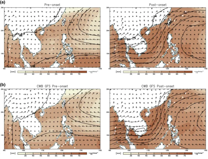
Following the circulation-based Uscs index (Wang et al. (2004); the pentad mean of average U-component wind speed at 850 hPa over 5°–15°N, 110°–120°E), the 2016 SCS summer monsoon onset is on May 20th, when the prevailing low-level wind switched from easterlies to intense and per-sistent southwesterly winds. The analysis period in this study consists of the pre- and post-onset periods, which are defined as 10 days before (5/10–19) and after (5/20–29) the onset date. The synoptic conditions for the pre- and post-onset period of the reanalysis data are shown in Fig. 1a, which demonstrate the sharp transition of large-scale circulation of the case, in terms of total precipitable water, horizontal wind fields and geopotential height at 850 hPa. In the pre-onset period, the SCS region is influenced by the subtropical ridge, which leads to a calm and dry environment in the region. In the post-onset period, the low-level trough is located in the
SCS region, accompanied with strong southwesterly winds and abundant moisture. A more suitable environment for organized convection’s occurrence in the SCS region is given in the post-onset period compared to the pre-onset period.
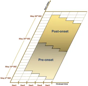
The ensemble members for our study are generated using the hindcast approach (Ma et al. 2013, 2015), in which the hindcasts are made daily at 00Z and integrated for 5 days from May 6th to May 29th. The initial condition datasets used for the total 24 hindcasts are made by the CWB data assimilation system. The first-day output of each hindcast are omitted, and the rest of the output is divided into the two analysis period according to their real time. The pre- (5/10–19) and post-onset (5/20–29) period have 40 days of output, respectively, and each day in real time has 4 days of output. The ensemble members are hindcasts initialized by the initial condition datasets of different dates, no other perturbation to the initial condition is added. The summary
Fig. 1 Average horizontal wind fields (vector) in m s−1 and average
geopotential height (contour) in m at 850 hPa and average total pre-cipitable water (shaded) of the a reanalysis and the, b hindcasts of the
pre-onset and post-onset period, respectively. The pre-onset period represents 5/10 to 5/19, and the post-onset period represents 5/20 to 5/29. All data are regridded onto a 0.25° grid
schematic diagram of our experiment design is presented in Fig. 2.
2.3 Observation and reanalysis datasets
The precipitation dataset used in this study is the Integrated Multi-satellitE Retrievals for Global Precipitation Measure-ment (IMERG V04) (Huffman et al. 2014). The IMERG provides precipitation estimates of half-hourly, 0.1° × 0.1° fields from 60°N to 60°S by combining data from all passive-microwave instruments in the Global Precipitation Measurement (GPM) constellation. The National Centers for Environment Prediction final operational global analysis data (NCEP GDAS/FNL 0.25) of six hourly, 0.25° × 0.25° fields (NCEP 2015) are used for synoptic analysis.
2.4 Object‑based precipitation system (OPS)
Tsai and Wu (2017) investigated the environment of aggre-gated deep convection using the idealized cloud-resolving simulations. They diagnosed the three-dimensional size of the cloud systems using a six-connected segmentation method, in which a cloud object is defined by connecting contiguous cloudy grids in 6 directions. This study uses the four-connected segmentation method as the analysis method, which is simplified from the six-connected segmentation method. Contiguous surface grid points where precipitation
intensity is stronger than 1 mm h−1 are connected and
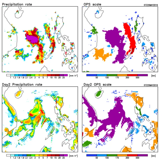
defined as a two-dimensional (x–y) object-based precipita-tion system (OPS). The OPSs are classified according to their horizontal size ranges, which is defined as the square root of the total area for each OPS. Xu et al. (2005, 2016) also use the equivalent diameter of objects as a measure of object size. The precipitation features associated with the OPS, such as spatial distribution, intensity spectrum, and diurnal variability can be investigated. A similar approach is also used to derive 2-D cloud pixels from satellite data (Wielicki and Welch 1986; Xu et al. 2005, 2016) and to diagnose radar echo size (Trivej and Stevens 2010). With the grey zone resolution, it is now feasible to analyze size ranges of OPSs in the GCMs and compare with observational sta-tistics. Figure 3 shows the schematic diagram of the OPS approach using a snapshot from the observation data and the model output. We note that the choice of the threshold intensity to identify OPS will influence the interpretation of the model bias if the threshold intensity is bigger than 1 mm h−1 because the excessive light rain in the model will
be masked out, which is one of the major model bias. The current results are not sensitive to the choice of the threshold intensity when it is smaller than 1 mm h−1.
3 Results
The synoptic conditions for the pre- and post-onset period of the hindcasts are shown in Fig. 1b. It can be seen that the synoptic conditions for both periods of the hindcasts are similar compared to the reanalysis data. Although some dis-crepancies can still be found between the hindcasts and the reanalysis data, the decent performance regarding the large-scale circulation of the 5-days hindcasts gives us enough confidence to further identify the precipitation bias associ-ated with the degree of convection organization and discuss the defects in the model physics.
3.1 Spatial distribution of OPS
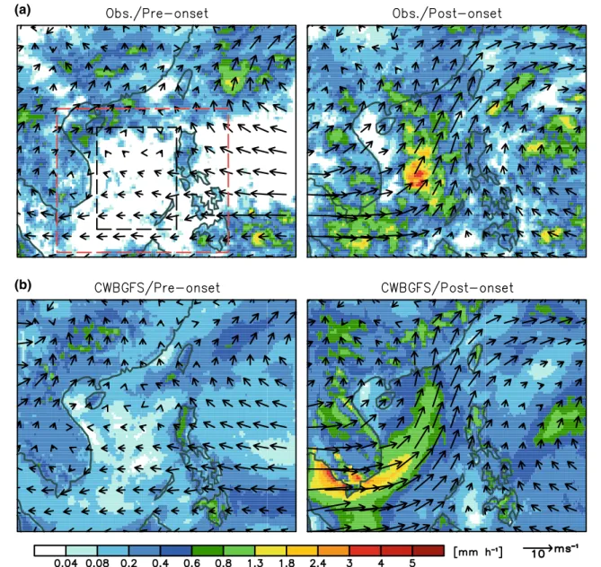
Figure 4 shows the spatial pattern of the average precipi-tation rate and 850 hPa horizontal wind fields of the pre- and post-onset periods of the 2016 SCS summer monsoon, respectively. In the observation (Fig. 4a), precipitation with the magnitude of 0.4 mm h−1 locates mostly over the land
areas surrounding SCS while there is almost no precipita-tion over the ocean during the pre-onset period. During the post-onset period, enhanced precipitation is found over the SCS under the strong southwesterly. Areas with intense pre-cipitation (around 4 mm h−1) are in the center of the SCS,
which is contributed by the tropical depression (WP012016, Joint Typhoon Warning Center). In the hindcasts (Fig. 4b), during the pre-onset period, weak precipitation spreads over
Fig. 2 The schematic diagram of our experiment design using the hindcast approach. The quadrilaterals in x-direction represent the dif-ferent integration time of the same hindcast. The first-day output of each hindcast are omitted, and rest of the output are separated into the two analysis periods according to their real time
broader areas in the SCS, and the surrounding land area has stronger precipitation that the intensity is around 0.6 (0.8) mm h−1 over Indochina (Philippines). During the
post-onset period, however, the precipitation hotspot over the SCS in the hindcasts is closer to Indochina, and its intensity (around 2.4 mm h−1) is weaker compared to the observation
(around 4 mm h−1). The land precipitation over Indochina
and Philippines are stronger in the hindcasts, with a narrow precipitation band along the coast of Indochina not seen in the observation.
The spatial distribution of precipitation associated with the size of OPS over SCS (the red dashed box in Fig. 4a) is shown in Fig. 5. In the observation, the precipitation
distributes sparsely, and the intensity increases with the increasing size of OPS when the OPS is smaller than 175 km during the pre-onset period. Overall the precipi-tation systems do not aggregate to OPS larger than 300 km during this period. Note that the precipitation contributed by OPS larger than 300 km near the Hainan Island is gen-erated by a frontal system which is propagated from out-side the SCS. During the post-onset period, the precipi-tation also distributes sparsely when the OPS is smaller than 175 km, while the precipitation systems aggregate toward the center of the SCS, and intensity of 1.5 mm−1
contributed by OPS larger than 500 km can be seen. In the
Fig. 3 The schematic diagram of the OPS approach. In the upper panel, the left figure is the snapshot of the precipitation rate of IMERG data at 07Z, May 25th, 2016, and the right figure is the snap-shot of the horizontal size range of OPS at the same time. The lower
panel shows the similar plots from the day2 hindcast at the same time as the observation. The horizontal size range represents the square root of the connected area
hindcasts, the precipitation over land is overestimated in the pre-onset period, and no precipitation contributed by OPS larger than 300 km can be seen in this period as well. During the post-onset period, the precipitation over land is also overestimated, and the precipitation intensity does not increase with the increasing size of OPS over the SCS. The intensity remains in the same order which is weaker than 0.3 mm h−1 when the OPS is smaller than 500 km.
Although the precipitation hotspot contributed by OPS larger than 500 km can still be seen in the hindcasts and their intensity is similar to the observation, the simulated precipitation is considered to be attributed to the accumu-lation of weak precipitation over an extended area within the post-onset period.
3.2 Precipitation intensity spectrum
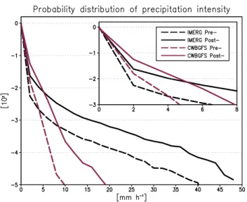
The observation and the hindcasts are interpolated to three hourly and 15 km in the following analysis regarding the precipitation intensity spectrum. Figure 6 shows the prob-ability density function (PDF) of the precipitation intensity over the SCS. For heavy precipitation, the observed intensi-ties of the probability < 10−3 (precipitation extreme stronger
than 99.9th percentile) are underestimated in the hindcasts for both the pre- and post-onset periods, showing that the bias exists under different environments. The inset in the upper right corner of Fig. 6 zooms in the range of intensity (0–8 mm h−1). The hindcasts overestimate the probability
of lighter rainfall (lower than 4 mm h−1 and 6 mm h−1 in
the pre- and post- onset period, respectively). Even with the
(a)
(b)
Fig. 4 Average precipitation rate (shaded) in mm h−1 of the a observation and the b hindcasts of the pre-onset and post-onset period,
horizontal resolution of ~ 15 km, the model still produces similar bias found by Stephens et al. (2010) in conventional GCMs with the grid size of O (100 km). Note that the opera-tional CWBGFS, which has the lower horizontal resolution (~ 25 km), also shows similar bias to the hindcasts here with higher resolution, and the comparison is shown in Appendix
A.
Figure 7 shows the PDF of areal fraction and the precipi-tation intensity spectrum related to the various size of OPS. The hindcasts overestimate the areal fraction of OPS with all size ranges, especially for those < 50 km and > 500 km. The observed intensities at 1st, 2nd, and 3rd quartiles all increase approximately linearly with the increase of OPS size. The intensity at higher percentiles increase even more substan-tially with size, and a sharp increase can be found at 99.99th
percentile, which increases from 30 to 45 m h−1 when the
size of OPS increases from 50 to 100 to 100–175 km. How-ever, the hindcasts underestimate the intensities at each percentile, and the positive relationship between the pre-cipitation extreme and the size of OPS is much weaker. The observation indicates that the OPS of 100 km is a thresh-old size ranges where the observed precipitation extreme increases sharply; however, the hindcasts do not exhibit such sensitivity, and the extreme precipitation intensity is under-estimated particularly for OPS with larger sizes.
3.3 Diurnal variability
The precipitation over the SCS has strong diurnal varia-tions with the apparent land-sea contrast (Yang and Slingo
Fig. 5 Average precipitation rate in mm h−1 of six size ranges of OPS in the pre- and post-onset periods of the observation and the hindcasts.
2001; Aves and Johnson 2008; Johnson 2011; Park et al.
2011; Mao and Wu 2012). The model bias can be associated with the representation in the diurnal cycle, which is shown in Fig. 8. During the pre-onset period, the hindcasts show a clear diurnal cycle over the land area peaking at 14 LT, which corresponds well with the observation. However, the diurnal amplitude over land (0.8 mm h−1) is overestimated
compared to the observation (0.4 mm h−1). Over the ocean,
the hindcasts overestimate the precipitation throughout the day. During the post-onset period, the observed diurnal amplitude over the land area increases to 0.8 mm h−1 and
the peak time delays to 17 LT. The simulated post-onset diurnal amplitude over land also increases but without delay in peak time. Over the ocean, the peak time is earlier in the hindcasts (02 LT) compared to the observation (08 LT), and the simulated diurnal amplitude (0.2 mm h−1) is weaker
compared to the observation (0.4 mm h−1).
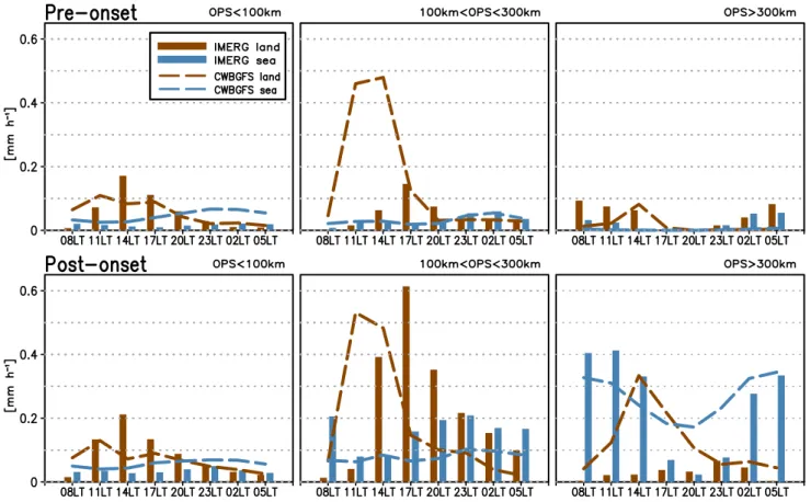
Figure 9 shows the diurnal variability of precipitation associated with the size of OPS. In the observation, the diurnal cycle of OPS smaller than 100 km over the land area peaks at 14 LT in both the pre- and post-onset periods, whereas the peak time of OPS with the size of 100–300 km delays to 17 LT during post-onset, well corresponding to the peak time of total precipitation over land. The OPS size exhibits a clear diurnal cycle over the ocean area after the monsoon onset. The precipitation over the ocean area con-tributed by OPS larger than 300 km maximizes in the morn-ing (08 LT to 11 LT) and minimizes in the evenmorn-ing (17 LT to 23 LT). However, these two features are both underrep-resented by the hindcasts. For OPS of 100–300 km over the land area, the diurnal peak time is earlier than the observa-tion for both periods, and the diurnal amplitude during the pre-onset period is highly overestimated. The precipitation contributed by OPS larger than 300 km over the land area in the post-onset period is also overestimated. Over the ocean, the precipitation contributed by OPS larger than 300 km in the post-onset period is overestimated in the evening, and the precipitation contributed by OPS smaller than 100 km are also overestimated in both periods.
4 Discussion
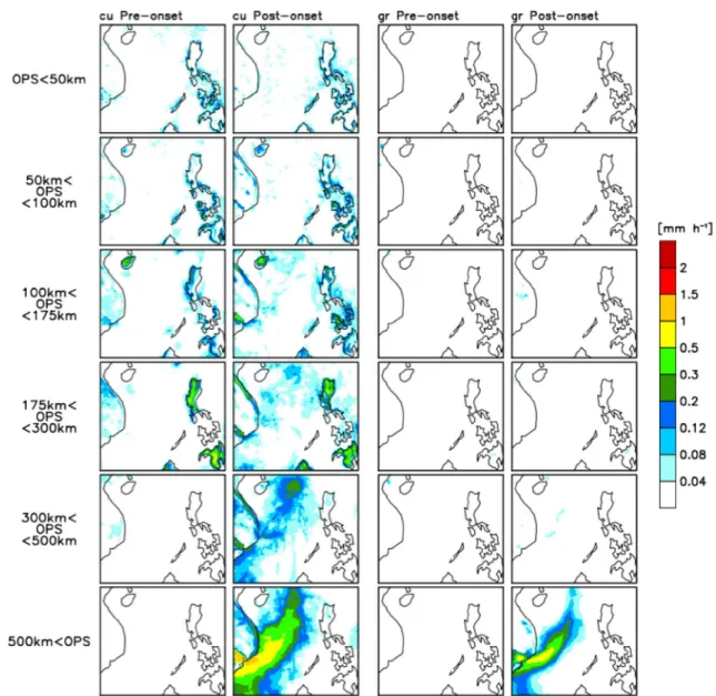
In the hindcasts, precipitation is produced from both sub-grid scale process (cumulus parameterization) and sub-grid-scale process (large scale condensation scheme). The precipitation produced by the two precipitating parameterizations is then analyzed respectively. Figure 10 shows the same figure as Fig. 5 but for the simulated precipitation contributed by the cumulus parameterization and the large-scale condensation scheme, respectively. It is found that almost all of the pre-cipitation is contributed by the cumulus parameterization, except the OPS larger than 500 km in the post-onset period. Therefore, the result also indicates that the cumulus param-eterization is responsible for the precipitation bias regarding diurnal variability.
The precipitation intensity spectrum of the different size range of OPS produced by cumulus parameterization and grid-scale condensation scheme respectively is then exam-ined (Fig. 7). It is found that the precipitation intensity
Fig. 6 The probability density function of precipitation intensity over the SCS region (the outer dashed box in Fig. 4a) in the pre- (dashed line) and post-onset (solid line) period of the observation (black line) and the hindcasts (maroon line). The interval of precipitation inten-sity is 2 mm h−1. The upper right figure zooms in the precipitation
intensity smaller than 8 mm h−1 with the same interval
Fig. 7 Probability density function of areal fraction (lower panel) and the 25th, 50th, 75th, 90th, 99th, 99.9th and 99.99th percentiles of precipitation rate (upper panel) of OPS with six size ranges over the SCS region in the observation (black) and the hindcasts (maroon) during the analysis period (5/10–5/29). The precipitation contributed by cumulus parameterization (sky blue), and large-scale condensation scheme (purple) is also shown. Different markers in the upper panel represent different percentiles of precipitation rate
spectrum produced by cumulus parameterization has nearly identical behavior among every size range of OPS, and the precipitation extremes are all below 10 mm h−1. On the other
hand, the precipitation extreme produced by the large-scale condensation scheme shows a large discrepancy between different size ranges of OPS. The precipitation extreme pro-duced by the large-scale condensation scheme stronger than 15 mm−1 can be seen in OPS of 50–100 km and OPS larger
than 300 km. However, it is still unknown how to present the observed relationship between precipitation intensity spec-trum and degree of convection organization in the model. The primary obstacle is the ambiguity of the precipitation partition between the two precipitating parameterizations.
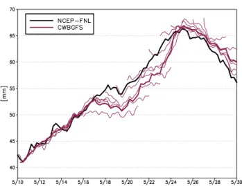
Besides the precipitation bias reported in this study, a dry bias over the SCS can be identified during the onset. Figure 11 shows the observed and simulated time series of
Fig. 8 Diurnal variability of average precipitation rate over the land (brown) and the ocean (blue) area of the SCS region of the observation (bar) and the hindcasts (dashed line) in the pre- and post-onset period, respectively
average column water vapor over the SCS (the black dashed box in Fig. 4a), and the results from individual hindcast member (which is initialized daily and integrated for 5 days) are also shown. During the onset, the observed column water vapor increases sharply from 5/10 (42 mm) to 5/25 (66 mm). The result from the hindcasts also represents the increase of moisture; however, a short period of moisture decrease is found during the onset. Starting from 5/17, the moisture in the hindcasts decrease from 53 to 51.5 mm in two days.
Meanwhile, the observed moisture remains the trend of increase. After the two days decreasing period, the moisture in the hindcasts return to the trend of moisture increase; nevertheless, the variation in moisture between the obser-vations and the hindcasts does not diminish until 5/23. The reason which causes the model drift is then investigated via analyzing the moisture budget over the SCS. We choose two
specific periods for the analysis: when the model drift starts (5/17–5/19), and when the dry bias persists (5/19–5/23).
Table 1 shows the moisture budget over the SCS of the observations and the hindcasts of the two periods. The mois-ture budget (Eq. 1) involves the change in total precipitable water (T), the vertically integrated moisture flux divergence (D), the evaporation (E), the precipitation (P), and the resid-ual term (R). For the observations, the evaporation (E) is calculated using the 0–3 h average surface latent heat flux from the forecast data of NCEP GDAS/FNL 0.25, and the precipitation (P) is calculated using the IMERG data, and the other terms are calculated using the reanalysis data.
During 5/17–5/19, the moisture divergence term in the hindcasts is smaller compared to the observations; however, (1) T + D = E − P + R
this is the period where the model starts to present a dry bias over the SCS. It can be seen that the dry bias is mostly contributed by the excessive precipitation, the precipita-tion produced by the hindcasts is almost twice as much as the observations. During 5/19–5/23, both the observations and the hindcasts present the increase of moisture, while the increase in the hindcasts is slightly smaller compared to the observations. In this period, the moisture convergence and the evaporation terms in the hindcasts are smaller, and the precipitation term is more significant compared to the observation.
It is found that the hindcasts produce much more pre-cipitation compared to the observations when the observed precipitation is small, while the hindcasts only produce slightly more precipitation when there is large precipitation in the observation. The result indicates that the production of precipitation in the model is more sensitive to the increase of moisture compared to the observation during the SCS summer monsoon onset. As shown in this study that the cumulus parameterization produces most of the simulated
precipitation in this case, it may also be responsible for the underrepresentation of the sensitivity of precipitation to moisture in the model.
With the high-horizontal resolution used in this study, we expect that the GCM can better represent the aggregation of the convective systems compared to the lower resolution GCMs. However, the evaluation method used in this study demonstrates that the precipitation bias increases when the convection is aggregated into a large system. This problem could be associated with model’s ability in representing con-vective systems through grid-scale processes. With the use of cumulus parameterization, the convective instability is first consumed through sub-grid scale processes leaving no room for the convective system to develop at the grid-scale. An additional closure for the cumulus parameterization that determines the amount of adjustment at a given environment could solve the problem for the grey zone GCMs. By physi-cally changing the partition between the grid-scale and the sub-grid scale processes, the model can better capture the isolated convection such as the afternoon thunderstorm with the sub-grid scale parameterization and the organized con-vection by the grid-scale processes. The closure assumption proposed by Arakawa and Wu (2013) and Wu and Arakawa (2014) provides the opportunity to represent the partition between grid-scale and sub-grid scale processes better. In Eq. (20) of Arakawa and Wu (2013), the vertical eddy transports by cumulus parameterization are adjusted by an additional parameter, λ. It is defined by the ratio between the grid-scale destabilization rate by the cumulus param-eterization and the cloud-environment difference of vertical velocity and moist static energy which depends on the cloud properties. When λ is large due to the large destabilization rate which represents the case for mesoscale convection, the subgrid parameterization is reduced. When λ is small for strong cloud updrafts which represent the case for iso-lated deep convection, the eddy transport is done mainly through the subgrid parameterization. This closure assump-tion, called unified parameterizaassump-tion, will be implemented in the following version CWBGFS, and the model bias will be evaluated using the analysis method presented in this study.
5 Summary
This study aims to evaluate the precipitation bias associ-ated with the degree of convection organization in the grey zone simulation of CWBGFS with parameterized convec-tion. By using the new analysis method, namely OPS, the relationship between the precipitation features (e.g., spatial distribution, spectrum, and diurnal variability) and the size of OPS are investigated. The selected case is the 2016 SCS summer monsoon onset, a period in which various types of convection occur.
Fig. 11 Time series of average column water vapor over SCS (black
dashed box in Fig. 4a) of the reanalysis (black line) and the hindcasts (thick maroon line). Thin maroon lines represent individual 5-day hindcasts
Table 1 Each term of the moisture budget equation over the SCS (the black dashed box in Fig. 4a) of the two periods and the unit is in mm. The meaning of the abbreviations is described in the context
T D E P R 5/17–5/19 Observations 1.83 2.36 5.70 2.84 1.33 Hindcasts − 1.31 1.06 5.20 5.29 − 0.16 5/19–5/23 Observations 7.43 − 10.20 17.70 19.14 − 1.33 Hindcasts 6.19 − 6.80 15.48 20.31 4.22
The result based on OPS shows that the observed precipi-tation tends to aggregate toward the center of the SCS after the SCS monsoon onset; precipitation intensity increases with the increase of OPS size. However, the increasing intensity with the increase of the OPS size is underrepre-sented by the hindcasts. Instead of aggregating toward the center of SCS, the precipitation in the hindcasts spreads more evenly over the region. The OPS of 100 km is a thresh-old size range where the observed precipitation extreme increase sharply; however, the hindcasts underrepresent the impact of aggregation on precipitation spectrum, especially for the extremes. The diurnal variability of precipitation is also found to be related to the degree of convection organiza-tion. Over land, the hindcasts cannot represent the observed delay in peak time with increasing OPS sizes. Over ocean during the post-onset period, the diurnal cycle amplitude of OPS larger than 300 km is underestimated. The evaluation of the precipitation bias associated with the size of OPS suggests that aggregation of the convective systems is not well represented in the CWBGFS with grey zone resolution, which is regarded as an essential objective to the improve-ment of CWBGFS in the future.
Acknowledgements This study is jointly supported by the Central Weather Bureau in Taiwan (1052281C, 1062221C), and the Ministry of Science and Technology in Taiwan (MOST-106-2111-M-002-005, MOST-106-2111-M-002-008, MOST-106-1502-02-11-01). We acknowledge the Central Weather Bureau providing the computa-tional resources for this work. The IMERG V04 data were provided by the NASA/Goddard Space Flight Center and PPS, which develop and compute the IMERG V04 as a contribution to GPM, and archived at ftp://arthu rhou.pps.eosdi s.nasa.gov/gpmda ta/ YYYY/MM/DD/imerg/ (accessed at 30 March 2017). The NCEP GDAS/FNL0.25 data were provided by the Computational and Information Systems Laboratory at the National Center for Atmospheric Research, and archived at https :// rda.ucar.edu/ datasets/ds083.3/ (accessed at 29 October 2017).
Appendix A
To demonstrate that the precipitation bias persists even with the increase in horizontal resolution, we compare the HR (higher resolution, ~ 15 km, which is used in the main text) and the operational CWBGFS (hereafter lower resolu-tion (LR), ~ 25 km) using four kinds of evaluaresolu-tion score. Table 2 shows the bias fraction, and the root mean square error (RMSE) over the SCS region in the pre- and post-onset periods in the HR and the LR. The bias fraction represents the ratio of temporal mean average precipitation rate over the SCS region (the outer dashed box in Fig. 4a) in the model to the observation, which could represent the precipitation bias in general. In the HR, the bias fraction in the pre-onset period (1.64) is more significant than the post-onset period (1.09), and their differences with the LR are small. The RMSE in the pre-onset period (0.64 mm h−1) is smaller than
the post-onset period (1.71 mm h−1), and their differences
with the LR are also small. The result shows that the model overestimates the precipitation during the onset, especially the pre-onset period. The RMSEs in the post-onset period are more significant than the pre-onset period, which is sup-posed to be caused by the underrepresentation of location and the intensity of the precipitation hotspot in the post-onset period.
Figure 12 shows the bias score and the equitable threat score (ETS) following Gustafson et al. (2014) over the SCS region in the HR and the LR in the pre- and post-onset period respectively. Both scoring methods define
Table 2 Bias fraction and root mean square error in the pre-onset and the post-onset period over the SCS region (the outer dashed box in Fig. 4a) of the HR and the LR
Bias fraction represents the ratio of temporal mean and spatial aver-age precipitation rate in the model to the observation. The data for analysis are interpolated to three hourly and 25 km
Pre-onset Post-onset Higher resolution
Bias fraction (unitless) 1.64 1.09 RMSE (mm h−1) 0.64 1.71
Lower resolution
Bias fraction (unitless) 1.68 1.10 RMSE (mm h−1) 0.65 1.73
(b) (a)
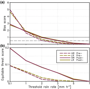
Fig. 12 a Bias scores and b equitable threat scores in the pre-onset
period (dashed line) and the post-onset period (solid line) over the SCS region of the HR (maroon line) and the CWBGFS with lower resolution (brown line).The data for analysis are interpolated to three hourly and 25 km. The x-axis represents the threshold rain rates. See more details in the context
precipitation event as where the precipitation rate exceeds a certain threshold. The bias score represents the ratio of the simulated event amount to the observed event amount, which is used to evaluate the precipitation area. The ETS is a more strictly test that the location of the event is also considered, which is defined as:
where
where nfo is amount of events both forecasted and observed, nfno is the number of events forecasted but not observed, nnfo
is the number of events observed but not forecasted, nf is
the number of events forecasted, no is the number of events
observed, and N is the number of total events which could occur.
In the HR, the bias score in the pre-onset period is higher (5) than the post-onset period (3) when the thresh-old is 0.1 mm h−1, and the bias score in the post-onset
period becomes higher compared with the score in the pre-onset period when the threshold increase. The result indicates that the HR overestimates the areas of light pre-cipitation mainly in the pre-onset period, and underesti-mates the areas of intense precipitation.
The highest ETS in the HR is found in the post-onset period when the threshold is 0.1 mm h−1, the value (0.2) is
similar to the result from Gustafson et al. (2014) which eval-uated the WRF model using CAM5 physics suite. The result somehow shows that the HR performs well in the post-onset period; however, the ETS in the pre-onset period is only 0.1. It can be seen that the ETS decreases with the increase in threshold in both periods, which shows that heavy precipi-tation is more difficult to forecast. In summary, the results from the four scoring methods all show that the precipitation bias persists with the increase in horizontal resolution.
References
Arakawa A (2004) The cumulus parameterization problem: past, present, and future. J Clim 17(13):2493–2525
Arakawa A, Wu CM (2013) A unified representation of deep moist convection in numerical modeling of the atmosphere. Part I. J Atmos Sci 70(7):1977–1992
Aves S, Johnson RH (2008) The diurnal cycle of convection over the northern South China Sea. J Meteorol Soc Jpn Ser II 86(6):919–934
Dai A, Trenberth KE (2004) The diurnal cycle and its depiction in the community Climate System Model. J Clim 17(5):930–951
(2) ETS = nfo −E(nfo) nfno+nnfo+nfo−E(nfo) (3) E(nfo ) = nfno N
Del Genio AD (2012) Representing the sensitivity of convective cloud systems to tropospheric humidity in general circulation models. Surveys Geophys 33(3–4):637–656
Derbyshire SH, Beau I, Bechtold P, Grandpeix JY, Piriou JM, Redelsperger JL, Soares PMM (2004) Sensitivity of moist con-vection to environmental humidity. Quart J R Meteorol Soc 130(604):3055–3079
Ek MB, Mitchell KE, Lin Y, Rogers E, Grunmann P, Koren V, … Tarpley JD (2003) Implementation of Noah land surface model advances in the National Centers for Environmental Prediction operational mesoscale Eta model. J Geophys Res: Atmos 108:D22 Fischer EM, Knutti R (2016) Observed heavy precipitation increase confirms theory and early models. Nat Clim Change 6(11):986 Flato G, Marotzke J, Abiodun B, Braconnot P, Chou SC, Collins WJ
et al (2013) Evaluation of climate models. In: climate change 2013: the physical science basis. Contribution of working group I to the fifth assessment report of the intergovernmental panel on climate change. Clim Change 2013 5:741–866
Gao J, Xue M, Stensrud DJ (2013) The development of a hybrid EnKF-3DVAR algorithm for storm-scale data assimilation. Adv Mete-orol 2013:512656. https ://doi.org/10.1155/2013/51265 6 Grabowski WW, Wu X, Moncrieff MW (1996) Cloud-resolving
mod-eling of tropical cloud systems during Phase III of GATE. Part I: Two-dimensional experiments. J Atmos Sci 53(24):3684–3709 Gustafson WI, Ma PL, Singh B (2014) Precipitation characteristics
of CAM5 physics at mesoscale resolution during MC3E and the impact of convective timescale choice. J Adv Model Earth Syst 6(4):1271–1287
Hamada A, Murayama Y, Takayabu YN (2014) Regional characteris-tics of extreme rainfall extracted from TRMM PR measurements. J Clim 27(21):8151–8169
Han J, Pan HL (2011) Revision of convection and vertical diffusion schemes in the NCEP global forecast system. Weather Forecast 26(4):520–533
Hortal M, Simmons AJ (1991) Use of reduced Gaussian grids in spec-tral models. Mon Weather Rev 119(4):1057–1074
Houze RA Jr (2004) Mesoscale convective systems. Rev Geophys 42:RG4003. https ://doi.org/10.1029/2004R G0001 50
Huffman G, Bolvin D, Braithwaite D, Hsu K, Joyce R, Xie P (2014) Integrated Multi-satellitE Retrievals for GPM (IMERG), version 4.4. NASA’s Precipitation Processing Center, accessed 30 March 2017
Iacono MJ, Delamere JS, Mlawer EJ, Shephard MW, Clough SA, Col-lins WD (2008) Radiative forcing by long-lived greenhouse gases: calculations with the AER radiative transfer models. J Geophys Res: Atmos 113:D13
Jeng BF, Chen HJ, Lin SC, Leou TM, Peng MS, Chang SW, … Chang CP (1991) The limited-area forecast systems at the Central Weather Bureau in Taiwan. Weather Forecast 6(1):155–180 Johnson RH (2011) Diurnal cycle of monsoon convection. In: The
global monsoon system: research and forecast, pp 257–276 Kessler E (1969) On the distribution and continuity of water substance
in atmospheric circulations. In: On the distribution and continuity of water substance in atmospheric circulations. American Mete-orological Society, Boston, pp 1–84
Khairoutdinov MF, Randall DA (2001) A cloud resolving model as a cloud parameterization in the NCAR Community Climate System Model: preliminary results. Geophys Res Lett 28(18):3617–3620 Kim D, Sobel AH, Maloney ED, Frierson DM, Kang IS (2011) A sys-tematic relationship between intraseasonal variability and mean state bias in AGCM simulations. J Clim 24(21):5506–5520 Kopparla P, Fischer EM, Hannay C, Knutti R (2013) Improved
simu-lation of extreme precipitation in a high-resolution atmosphere model. Geophys Res Lett 40(21):5803–5808
Li W, Luo C, Wang D, Lei T (2010) Diurnal variations of precipitation over the South China Sea. Meteorol Atmos Phys 109(1–2):33–46
Liou CS, Chen JH, Terng CT, Wang FJ, Fong CT, Rosmond TE, Kuo HC, Shiao CH, Cheng MD (1997) The second–generation global forecast system at the central weather bureau in Taiwan. Weather Forecast 12(3):653–663
Liu YC, Fan J, Zhang GJ, Xu KM, Ghan SJ (2015) Improving repre-sentation of convective transport for scale-aware parameterization: 2. Analysis of cloud-resolving model simulations. J Geophys Res: Atmos 120(8):3510–3532
Liu YC, Fan J, Xu KM, Zhang GJ (2018) Analysis of cloud-resolving model simulations for scale dependence of convective momentum transport. J Atmos Sci 75:2445–2472. https ://doi.org/10.1175/ JAS-D-18-0019.1
Ma HY, Xie S, Boyle JS, Klein SA, Zhang Y (2013) Metrics and diag-nostics for precipitation-related processes in climate model short-range hindcasts. J Clim 26(5):1516–1534
Ma HY, Chuang CC, Klein SA, Lo MH, Zhang Y, Xie S, … Phillips TJ (2015) An improved hindcast approach for evaluation and diagno-sis of physical processes in global climate models. J Adv Model Earth Syst 7(4):1810–1827
Mao J, Wu G (2012) Diurnal variations of summer precipitation over the Asian monsoon region as revealed by TRMM satellite data. Sci China Earth Sci 55(4):554–566
Mapes BE, Bacmeister JT (2012) Diagnosis of tropical biases and the MJO from patterns in the MERRA analysis tendency fields. J Clim 25(18):6202–6214
Moncrieff MW (2004) Analytic representation of the large-scale organ-ization of tropical convection. J Atmos Sci 61(13):1521–1538 Moncrieff MW, Klinker E (1997) Organized convective systems
in the tropical western pacific as a process in general circula-tion models: a toga coare case-study. Quart J R Meteorol Soc 123(540):805–827
National Centers for Environmental Prediction/National Weather Ser-vice/NOAA/U.S. Department of Commerce (2015) updated daily. NCEP GDAS/FNL 0.25 Degree Global Tropospheric Analyses and Forecast Grids. Research Data Archive at the National Center for Atmospheric Research, Computational and Information Sys-tems Laboratory. Accessed 29 October 2017
Palmer TN, Shutts GJ, Swinbank R (1986) Alleviation of a systematic westerly bias in general circulation and numerical weather predic-tion models through an orographic gravity wave drag parametriza-tion. Quart J R Meteorol Soc 112(474):1001–1039
Park MS, Ho CH, Kim J, Elsberry RL (2011) Diurnal circulations and their multi-scale interaction leading to rainfall over the South China Sea upstream of the Philippines during intraseasonal mon-soon westerly wind bursts. Clim Dyn 37(7–8):1483–1499 Peng MS, Jeng BF, Chang CP (1993) Forecast of typhoon motion in
the vicinity of Taiwan during 1989–90 using a dynamical model. Weather Forecast 8(3):309–325
Ploshay JJ, Lau NC (2010) Simulation of the diurnal cycle in tropical rainfall and circulation during boreal summer with a high-resolu-tion GCM. Mon Weather Rev 138(9):3434–3453
Sanderson BM, Shell KM, Ingram W (2010) Climate feedbacks deter-mined using radiative kernels in a multi-thousand member ensem-ble of AOGCMs. Clim Dyn 35(7–8):1219–1236
Scinocca JF (2003) An accurate spectral nonorographic gravity wave drag parameterization for general circulation models. J Atmos Sci 60(4):667–682
Stephens GL, L’Ecuyer T, Forbes R, Gettelmen A, Golaz JC, Bodas-Salcedo A, … Haynes J (2010) Dreary state of precipitation in global models. J Geophys Res: Atmos 115:D24
Trivej P, Stevens B (2010) The echo size distribution of precipitating shallow cumuli. J Atmos Sci 67(3):788–804
Tsai WM, Wu CM (2017) The environment of aggregated deep convec-tion. J Adv Model Earth Syst 9(5):2061–2078
Wang B, Zhang Y, Lu MM (2004) Definition of South China Sea soon onset and commencement of the East Asia summer mon-soon. J Clim 17(4):699–710
Wielicki BA, Welch RM (1986) Cumulus cloud properties derived using Landsat satellite data. J Clim Appl Meteorol 25(3):261–276 Willetts PD, Marsham JH, Birch CE, Parker DJ, Webster S, Petch J
(2017) Moist convection and its upscale effects in simulations of the Indian monsoon with explicit and parametrized convection. Quart J R Meteorol Soc 143(703):1073–1085
Wu CM, Arakawa A (2014) A unified representation of deep moist convection in numerical modeling of the atmosphere. Part II. J Atmos Sci 71(6):2089–2103
Xu KM, Randall DA (1996) A semiempirical cloudiness parameteriza-tion for use in climate models. J Atmos Sci 53(21):3084–3102 Xu KM, Wong T, Wielicki BA, Parker L, Eitzen ZA (2005)
Statisti-cal analyses of satellite cloud object data from CERES. Part I: Methodology and preliminary results of the 1998 El Niño/2000 La Niña. J Clim 18(13):2497–2514
Xu KM, Wong T, Dong S, Chen F, Kato S, Taylor PC (2016) Cloud object analysis of CERES aqua observations of tropical and subtropical cloud regimes: four-year climatology. J Clim 29(5):1617–1638
Yang GY, Slingo J (2001) The diurnal cycle in the tropics. Mon Weather Rev 129(4):784–801
Yun Y, Fan J, Xiao H, Zhang GJ, Ghan SJ, Xu KM, … Gustafson WI (2017) Assessing the resolution adaptability of the Zhang-McFarlane cumulus parameterization with spatial and temporal averaging. J Adv Model Earth Syst 9(7):2753–2770
Zhang GJ, Fan J, Xu KM (2015) Comments on “A unified representa-tion of deep moist convecrepresenta-tion in numerical modeling of the atmos-phere. Part I”. J Atmos Sci 72(6):2562–2565
Zhao Q, Carr FH (1997) A prognostic cloud scheme for operational NWP models. Mon Weather Rev 125(8):1931–1953
Publisher’s Note Springer Nature remains neutral with regard to jurisdictional claims in published maps and institutional affiliations.