Fuzzy data mining for interesting generalized association rules

The fuzzy data mining generalized

association rules for quantitative values

Tzung-Pei Hong* and Kuei-Ying Lin

Graduate School of Information Engineering I-Shou University

Kaohsiung, 84008, Taiwan, R.O.C. {tphong, m883331m}@ isu.edu.tw

Abstract

Due to the increasing use of very large databases and data warehouses, mining useful information and helpful knowledge from transactions is evolving into an important research area. Most conventional data-mining algorithms identify the relationships among transactions using binary values and find rules at a single concept level. Transactions with quantitative values and items with hierarchy relation are, however, commonly seen in real-world applications. In this paper, we introduce the problem of mining generalized association rules for quantitative values. We propose fuzzy generalized rules mining algorithm for extracting implicit knowledge from transactions stored as quantitative values. Given a set of transaction and predefined taxonomy, we want to find fuzzy generalized association rules where the quantitative of items may be from any level of the taxonomy. Each item uses only the linguistic term with the maximum cardinality in later mining processes, thus making the number of fuzzy regions to be processed the same as that of the original items. The algorithm can therefore focus on the most important linguistic terms and reduce its time complexity. We propose algorithm combines fuzzy transaction data mining algorithm and mining generalized association rules algorithm. This paper related to set concepts,

fuzzy data mining algorithms and taxonomy and generalized association rules.

Keywords: fuzzy data mining, fuzzy set, generalized association rule, quantitative value, taxonomy.

--- * Corresponding author

1.

Introduction

As the information technology (IT) has progressed rapidly, the capability of

storing and managing data in databases is becoming important. Though the IT

development facilitates data processing and eases spending of storage medium,

extraction of implicitly available information to aid decision making becomes a new

challenging work. Efficient mechanisms for mining information and knowledge from

large databases have thus been designed vigorously. As the results, data mining, first

proposed by Agrawal et al. in 1993 [1], becomes a central study field in both

databases and artificial intelligence.

Finding association rules from transaction databases is most commonly seen in

data mining [1][2][3][7][11][12][13][15][16][26]. It discovers relationships among

items such that the presence of some items in a transaction would imply the presence

of other items. The application of association rules is very wide. For example, they

could be used to inform managers in a supermarket what items (products) customers

would like to buy together, thus be useful for planning and marketing activity

[1][2][6]. More concretely, assuming that an association rule “if one customer buys

place the milk near the bread area to inspire customers to purchase them at once.

Additionally, the manager can promote the milk and the bread by packing them

together on sale so as to earn good profits for the supermarket.

Most previous studies have mainly shown how binary valued transaction data

may be handled. Transaction data in real-world applications however usually consist

of quantitative values, so designing a sophisticated data-mining algorithm able to deal

with quantitative data presents a challenge to workers in this research field.

In the past, Agrawal and his co-workers proposed several mining algorithms

based on the concept of large itemsets to find association rules in transaction data

[1-3]. They also proposed a method [26] for mining association rules from data sets

with quantitative and categorical attributes. Their proposed method first determines

the number of partitions for each quantitative attribute, and then maps all possible

values of each attribute into a set of consecutive integers. Some other methods were

also proposed to handle numeric attributes and to derive association rules. Fukuda et

al introduced the optimized association-rule problem and permitted association rules

to contain single uninstantiated conditions on the left-hand side [13]. They also

values of the rules are maximized. However, their schemes were only suitable for a

single optimal region. Rastogi and Shim thus extended the problem for more than one

optimal region, and showed that the problem was NP-hard even for the case of one

uninstantiated numeric attribute [23][24].

Fuzzy set theory is being used more and more frequently in intelligent systems

because of its simplicity and similarity to human reasoning [20]. Several fuzzy

learning algorithms for inducing rules from given sets of data have been designed and

used to good effect with specific domains [4-5, 6, 10, 14, 17-19, 25, 28-29]. Strategies

based on decision trees were proposed in [8-9, 21-22, 25, 30-31], and Wang et al.

proposed a fuzzy version space learning strategy for managing vague information [28].

Hong et al also proposed a fuzzy mining algorithm for managing quantitative data

[16].

Basically, this approach applies the fuzzy concepts in the Taxonomy information

to discover useful fuzzy generalized association rules among quantitative values. The

goal of data mining is to discover important associations among items such that the

presence of some items in a transaction will imply the presence of some other items.

To achieve this purpose, we proposed this method that combine FTDA algorithm [16]

concepts of fuzzy sets and the Apriori algorithm to find interesting itemsets and fuzzy

association rules from transaction data, the algorithm called FTDA(fuzzy transaction

data-mining algorithms). The algorithm is specially capable of transforming

quantitative values in transactions into linguistic terms, then filtering them, picking

them up and associating them using modified Apriori algorithm. The FTDA algorithm

can thus consider the implicit information of quantitative values in the transactions

and can infer useful association rules from them. Ramakrishnan Srikant and Rakesh

Agrawal introduce the problem of mining generalized association rules. Given a large

database of transaction, where each transaction consists of a set of items, Taxonomy

(is-a hierarchy) on the items, we find generalized associations rules between items at

any level of Taxonomy.

The remaining parts of this paper are organized as follows. Mining generalized

association rules for quantitative values at taxonomy is introduced in Section 2.

Fuzzy-set concepts are reviewed in Section 3. Notation used in this paper is defined in

Section 4. A new fuzzy data mining generalized association rules algorithm is

proposed in Section 5. An example to illustrate the proposed algorithm is given in

Section 6. Discussion and conclusions are finally stated in Section 7.

Our algorithm combines fuzzy transaction data-mining algorithm (called FTEA algorithm) that proposed by Tzung-Pei Hong et al [16] and “generalized association rule ” that proposed by Ramakrishnan Srikant and Rakesh Agrawal[27]. Our algorithm includes fuzzy set, fuzzy data mining, generalized association rules and

predefined taxonomy. Explain generalized association rules and predefined

taxonomy concepts in this section.

In mining generalized association rules, the problem of mining generalized association rules. Informally, given a set of transaction and predefined taxonomy, we want to find association rules where the items may be from any level of the taxonomy.

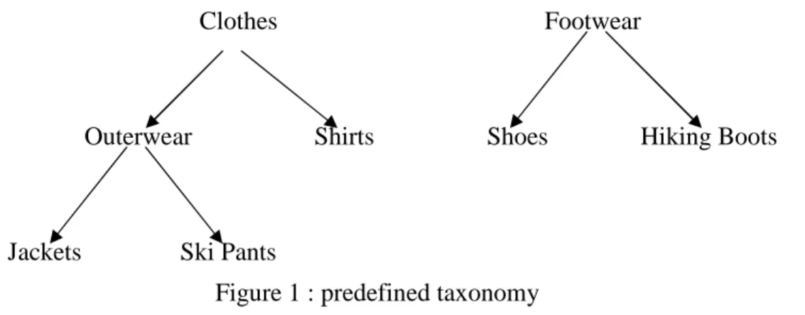
Figure 1 : predefined taxonomy

In most cases, taxonomies (is-a hierarchies) over the items are available. An example of predefined taxonomy is shown in Figure 1: this taxonomy says that Jacket is-a Outerwear. Ski Pants is-a Outerwear. Outerwear is-a Clothes, etc. Users are interested in generating rules that span different levels of the taxonomy. For example, we may infer a rule that people who buy Outerwear tend to buy Hiking Boots from the fact that people bought Jackets with Hiking Boots and Ski Pants with Hiking Boots. However, the support for the rule “Outerwear ⇒ Hiking Boots” may not be the sum

Clothes

Outerwear Shirts

Jackets Ski Pants

Footwear

of the supports for the rules “Jackets ⇒ Hiking Boots” and “Ski Pants ⇒ Hiking Boots” since some people may have bought Jackets. Ski Pants and Hiking Boots in the same transaction. Also, “Outerwear ⇒ Hiking Boots” may be a valid rule, while “Jackets ⇒ Hiking Boots” and “Clothes ⇒ Hiking Boots” may not. The former may not have minimum support, and the latter may not have minimum confidence.

Previous work on quantifying the “usefulness” or “interest” of a rule focused on how much the support of a rule was more than the expected support based on the support of the antecedent and consequent. Piatetsly-Shapiro argues that a rule X Y is not interesting if support (X Y) ≈ support (X) * support (Y). This measure did not prune many rules. We have a problem that the rules were found to be redundant. We use the information in taxonomy to derive a new interest measure that prunes out 40% to 60% of the rules as “redundant” rules.

Consider the rule:

Clothes Footwear (8% support, 75% confidence)

If “Clothes” is a parent of “Shirts”, and about a half of sales of “Clothes” are “Shirts”, we would expect the rule:

Shirts Footwear (4% support, 75% confidence)

The rules can be considered redundant since it does not convey any additional information and is less general than the first rule. The notion of “interest” by saying that we only want to find rules whose support is more than R times the expected value or whose confidence is more than R times the expected value, for some user-specified constant R. We say that an rule is interesting if it has no ancestors or it is R- interesting whit respect to its close ancestors among its interesting ancestors.

3. Review of Fuzzy Set Concepts

Fuzzy set theory was first proposed by Zadeh and Goguen in 1965 [32]. Fuzzy

set theory is primarily concerned with quantifying and reasoning using natural

language in which words can have ambiguous meanings. This can be thought of as an

extension of traditional crisp sets, in which each element must either be in or not in a

set.

Formally, the process by which individuals from a universal set X are determined

to be either members or non-members of a crisp set can be defined by a characteristic

or discrimination function [32]. For a given crisp set A, this function assigns a value

µ

_





µ

Thus, the function maps elements of the universal set to the set containing 0 and

1. This kind of function can be generalized such that the values assigned to the

elements of the universal set fall within specified ranges, referred to as the

of set membership. Such a function is called the membership function,

µ

which a fuzzy set A is usually defined. This function is represented by

µ

where [0, 1] denotes the interval of real numbers from 0 to 1, inclusive. The

function can also be generalized to any real interval instead of [0,1].

A special notation is often used in the literature to represent fuzzy sets. Assume

that x1 to xn are the elements in fuzzy set A, and µ1 to µn are, respectively, their grades of membership in A. A is then usually represented as follows:

A=µ1/x1+µ2/x2+...+µn/xn.

An

α

of

α

The scalar cardinality of a fuzzy set A defined on a finite universal set X is the

summation of the membership grades of all the elements of X in A. Thus,

A _A x

x X = ∑

∈ µ ( ) .

Among operations on fuzzy sets are the basic and commonly used

complementation, union and intersection, as proposed by Zadeh.

(1) The complementation of a fuzzy set A is denoted by

¬

membership function of ¬A is given by:

µ¬A ( )x = −1 µ¬A ( )x , ∀ ∈x X .

(2) The intersection of two fuzzy sets A and B is denoted by A I B, and the

membership function of A I B is given by:

µ

{

µ

µ

}

x x x

I ( ) min= ( ) , ( ) , ∀ ∈x X .

(3) The union of fuzzy sets A and B is denoted by A U B, and the membership

µ

{

µ

µ

}

x x x

∪ ( ) max= ( ) , ( )

The above concepts will be used in our proposed algorithm to mine fuzzy

association rules at predefined taxonomy.

4. Notation

The following notation is used in our proposed algorithm:

n: the total amount of transaction data;

mk: the total number of attributes at level k;

l: the total number of level in the predefined taxonomy

i

D : the i-th transaction datum, 1≤i≤n; k

j

I : the j-th group name at level k, 1≤j≤mk,1≤k≤l; h: the number of fuzzy regions forIkj ;

k jc

R : the k-th fuzzy region ofIkj , 1≤c≤h; k

ij

v : the quantitative value ofIkj at level k in the transaction Di;

k ij

f

ijc

jc

count : the summation of f_ijck, i=1 to n;

max-count : the maximum count value among j count values, c=1 to h; jc

max-R : the fuzzy region of _j Ik_j with max-count ; _j

α

λ

Cr: the set of candidate itemsets with r attributes (items);

r

L : the set of large itemsets with r attributes (items).

5. The fuzzy data mining generalized association rule

algorithm

The proposed fuzzy mining algorithm first uses membership functions to

transform each quantitative value into a fuzzy set in linguistic terms. The algorithm

then calculates the scalar cardinalities of all linguistic terms in the transaction data.

Each attribute uses only the linguistic term with the maximum cardinality in later

mining processes, thus keeping the number of items the same as that of the original

attributes. The algorithm is therefore focused on the most important linguistic terms,

which reduces its time complexity. The mining process using fuzzy counts is then

are described below.

The mining fuzzy generalized rule algorithm:

INPUT: A body of n transaction data, each with m attribute values, a set of

membership functions, a predefined minimum support valueα, and a

predefined confidence valueλ.

OUTPUT: A set of fuzzy association rules.

STEP 1: Group the items with the predefined taxonomy in each transaction datum Di,

and calculate the total item amount in each group. Let the amount of the j-th group name at level k in transaction Di be denoted

k ij

v .

STEP 2: Transform the quantitative valuev_ijk of each transaction datum Di, i=1 to n,

for each appearing encoded group name Ik_j , into a fuzzy set f_ijk

represented as _       + + + _k jh k ijh k j k ij k j k ij R f R f R f .... 2 2 1 1

using the given membership

functions, where h is the number of fuzzy regions for Ik_j, k jl

R is the l-th

fuzzy region of Ik_j, 1≤l≤h, and f_ijck isv_ijk’s fuzzy membership value in

regionRk_jc.

STEP 3: Calculate the scalar cardinality of each fuzzy region Rk_jc in the transaction

∑

STEP 4: Find max-

(

)

h c j MAX count count 1 =

= , for j= 1 to m. Let max-R _j be the region with max- count _j for item Ik_j . The region max-R _j will be used to

represent the fuzzy characteristic of this item Ik_j in later mining processes.

STEP 5: Check whether the value max-count _j of a region max- R _j , j=1 to m, is

larger than or equal to the predefined minimum support value α . If a region

max-R is equal to or greater than the minimum support value, put it in the _j

large 1-itemsets (L ). That is, 1

{

}

L₁ = max− _j max− _j ≥

α

STEP 6: Generate the candidate set C2 from L1. Each 2-itemset in C2 must not

ancestor or descendant relation in the taxonomy. All the possible 2-itemsets

are collected as C2.

STEP 7: Do the following substeps for each newly formed candidate 2-itemset s with

items (s1, s2) in C2.

(a) Calculate the fuzzy value of s in each transaction datum D_i as

2 1 is is is f f f = Λ , where j is

f is the membership value of D_i in region sj. If

the minimum operator is used for the intersection, then fis =min(fis1,fis2). (b) Calculate the scalar cardinality of s in the transaction data as:

counts=

∑

(c) If counts is larger than or equal to the predefined minimum support value

α

put s in L2.

STEP 8: Set r=2, where r is used to represent the number of items kept in the current

large itemsets.

STEP 9: IF L2 is null, then have no any rule in these transaction data; otherwise, do

the next step.

STEP 10: Generate the candidate set Cr+1 from Lr in a way similar to that in the

apriori algorithm [4]. The items of candidate set are not ancestor or

descendant relation. That is, the algorithm first joins Lr and Lr assuming that

r-1 items in the two itemsets are the same and the other one is different. It

then keeps in Cr+1 the itemsets, which have all their sub-itemsets of r items

existing in Lr.

STEP 11: Do the following substeps for each newly formed (r+1)-itemset s with items

(

s

,

s

,

...,

s

)

(a) Calculate the fuzzy value of s in each transaction datum D_i as

1 2 1

Λ

Λ

...

Λ

=

f

f

f

f

f is the membership value of D_i

in region sj. If the minimum operator is used for the intersection,

then is_j r j is

Min

f

f

=

(b) Calculate the scalar cardinality of s in the transaction data as: counts =

∑

(c) If counts is larger than or equal to the predefined minimum support value

α

put s in Lr+1.

STEP 12: If Lr+1 is null, then do the next step; otherwise, set r=r+1 and repeat STEPs

10 to 12.

STEP 13: Construct the association rules for all large q-itemset s with items

(

)

(a) Form all possible association rules as follows:

s1Λ...Λs_k−1Λs_k+1Λ...Λs_q → s_k, k=1 to q.

(b) Calculate the confidence values of all association rules using the formula:

∑

∑

STEP 14: Check the confidence values larger than or equal to the predefined

confidence thresholdλ.

STEP 15: Output the interesting rules with have different consequent or antecedent no

ancestor or descendant relation in the taxonomy or different linguistic

17

After STEP 15, the rules output can serve as meta-knowledge concerning the given transactions.

6. Example

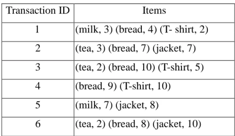
In the section, an example id given to illustrate the proposed generalized fuzzy data mining algorithm for quantitative values. This is a simple to show the proposed algorithm can be used to generate generalized association rules form quantitative transaction using predefined taxonomy. The set of data, including 6 transaction, are shown in table 1.

Table 1. Five transactions in this example

Transaction ID Items

1 (milk, 3) (bread, 4) (T- shirt, 2) 2 (tea, 3) (bread, 7) (jacket, 7) 3 (tea, 2) (bread, 10) (T-shirt, 5) 4 (bread, 9) (T-shirt, 10)

5 (milk, 7) (jacket, 8)

6 (tea, 2) (bread, 8) (jacket, 10)

Each transaction includes a transaction ID and some items bought. Each

item is represented by a tuple (item name, item amount). For example, the fourth

transaction consists of nine units of bread and ten units of T-shirt. Assume the

predefined taxonomy is shown in Figure 2.

Food

Brink bread

18

Figure 2. the predefined taxonomy in this example

In Figure 2, Food, brink and cloth are grouped name. Food can be classified into

two classes: brink and bread. Brink can be further classified into milk and tea, cloth

can be classified into jacket and T-shirt. We can use coed to represent items and

grouped name. For example, code A represent milk and B represent tea. Results are

shown in Figure 3.

Figure 3 the predefined taxonomy using code in this example

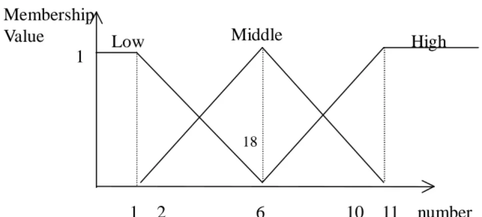
Also assume that the fuzzy membership functions are the same for all the items

and are as shown in Figure 4. T2

T1 C

A B

T3

D E

Low Middle High

Membership Value

Figure 4. The membership functions used in this example

In this example, amounts are represented by three fuzzy regions: Low, Middle

and High. Thus, three fuzzy membership values are produced for each item amount

according to the predefined membership functions. For the transaction data in Table 1,

the proposed fuzzy mining algorithm proceeds as follows.

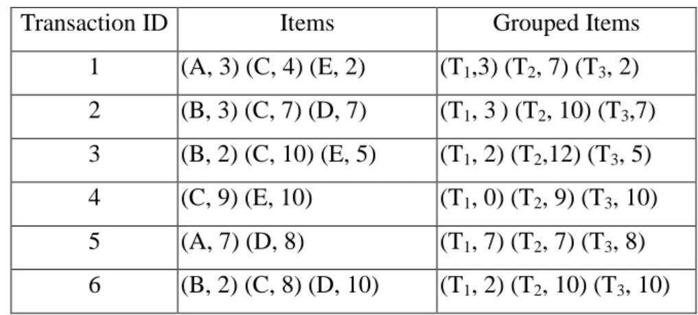
STEP 1: All the items in the transactions are first grouped. Take the items in

transaction T1 as an example. The items (A, 3) is grouped into (T1, 3); (A, 3) and (C,

4) are grouped into (T2, 7); (E, 2) is grouped into (T3, 2). Results for all the

transaction data are shown in Table 2.

Table 2 the set of items and grouped items

Transaction ID Items Grouped Items

1 (A, 3) (C, 4) (E, 2) (T1,3) (T2, 7) (T3, 2) 2 (B, 3) (C, 7) (D, 7) (T1, 3) (T2, 10) (T3,7) 3 (B, 2) (C, 10) (E, 5) (T1, 2) (T2,12) (T3, 5) 4 (C, 9) (E, 10) (T1, 0) (T2, 9) (T3, 10) 5 (A, 7) (D, 8) (T1, 7) (T2, 7) (T3, 8) 6 (B, 2) (C, 8) (D, 10) (T1, 2) (T2, 10) (T3, 10)

Take the first item in transaction T4 as an example. The amount “7”of D is converted

into a fuzzy set )

4 . 0 6 . 0 0 . 0 ( High Middle

Low+ + using the given membership functions (Figure 4).

This step is repeated for the other items, and the results are shown in Table 3, where

the notation item.term is called a fuzzy region.

Table 3. fuzzy sets transformed from the data in Table 2

TID Level-1 fuzzy set

T1 ₎ . 2 . 0 . 8 . 0 )( . 2 . 0 . 8 . 0 )( . 4 . 0 . 6 . 0 )( . 2 . 0 . 8 . 0 )( . 6 . 0 . 4 . 0 )( . 4 . 0 . 6 . 0 ( 3 3 2 2 1

1Low TMiddle T Middle T High T Low T Middle

T Middle E Low E Middle C Low C Middle A Low A + + + + + + T2 ) . 2 . 0 . 8 . 0 )( . 8 . 0 . 2 . 0 )( . 4 . 0 . 6 . 0 )( . 2 . 0 . 8 . 0 )( . 2 . 0 . 8 . 0 )( . 4 . 0 . 6 . 0 ( 3 3 2 2 1

1Low T MiddleT Middle T High T Middle T High

T High D Middle D High C Middle C Middle B Low B + + + + + + T3 ) . 8 . 0 . 2 . 0 )( . 0 . 1 )( . 2 . 0 . 8 . 0 )( . 8 . 0 . 2 . 0 )( . 2 . 0 . 8 . 0 )( . 2 . 0 . 8 . 0 ( 3 3 2 1

1Low T Middle T High T Low T Middle

T Middle E Low E High C Middle C Middle B Low B + + + + + T4 ₎ . 8 . 0 . 2 . 0 )( . 6 . 0 . 4 . 0 ))( . 8 . 0 . 2 . 0 )( . 6 . 0 . 4 . 0 ( 3 3 2

2Middle T High T Middle T High

T High E Middle E High C Middle C + + + + T5 ₎ . 4 . 0 . 6 . 0 )( . 2 . 0 . 8 . 0 )( . 2 . 0 . 8 . 0 )( . 4 . 0 . 6 . 0 )( . 2 . 0 . 8 . 0 ( 3 3 2 2 1

1Middle THigh T Middle T High T Middle T High

T High D Middle D High A Middle A + + + + + T6 ) . 8 . 0 . 2 . 0 )( . 8 . 0 . 2 . 0 )( . 2 . 0 . 8 . 0 )( . 8 . 0 . 2 . 0 )( . 4 . 0 . 6 . 0 )( . 2 . 0 . 8 . 0 ( 3 3 2 2 1

1Low T MiddleT Middle T High T Middle T High

T High D Middle D High C Middle C Middle B Low B + + + + + +

STEP 3: The scalar cardinality of each fuzzy region in the transactions is

calculated as the count value. Take the fuzzy region C.High as an example. Its scalar

cardinality = (0.0 + 0.2 + 0.2 + 0.6 + 0.0 + 0.4) = 1.4. This step is repeated for the

other regions, and the results are shown in Table 4.

Table4. The counts of the items regions

Item Count Item Count Item Count Item Count A.Low 0.6 C.Low 0.4 E.Low 0.4 T2.Low 0.6 A.Midlle 1.2 C.Midlle 3.2 E.Midlle 1.4 T2.Midlle 1.2 A.High 0.2 C.High 1.2 E.High 2.4 T .High 0.2

B.Low 2.2 D.Low 0.0 T1.Low 0.4 T3.Low 0.6 B.Midlle 0.8 D.Midlle 1.6 T1.Midlle 2.4 T3.Midlle 2.2 B.High 0.0 D.High 1.4 T1.High 1.2 T3.High 0.2

STEP 4. The fuzzy region with the highest count among the three possible

regions for each item is found. Take the item ‘A’ as an example. The count is 0.6 for

Low, 1.2 for Middle, and 0.2 for High. Since the count for Middle is the highest

among the three counts, the region Middle is thus used to represent the item ‘A’ in

later mining processes. This step is repeated for the other items, "Low" is chosen for B

and T1, “Middle” is chosen for C, D, E and T3, "High" is chosen T2.

STEP 5. The count of any region kept in STEP 4 is checked for a predefined

minimum support value α . Assume in this example,α is set at 1.7. Since all the

count values of B.Low, C.Middle, T1.Low, T2.High and T3.Middle are larger than 1.7,

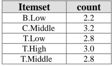
these items are put in L1 (Table 5).

Table 5. The set of large 1-itemsets in this example

Itemset

count

ancestor or descendant relation in the taxonomy as follows: (B.Low, C.Middel), (B.Low, T3.Middel), (C.Middel, T1.Middel), (C.Middel, T3.Middel), (T1.Middel, T3.Middel), (T2.High, T3.Middel).

STEP 7. The following substeps are done for each newly formed candidate 2-itemset

in C2:

(a) The fuzzy membership values of each transaction data for the

candidate 2-itemsets are calculated. Here, the minimum operator is used

for intersection. Take (B.Low, C.Middle) as an example. The derived

membership value for transaction 2 is calculated as : min(0.6, 0.8)=0.6.

The results for the other transaction are shown in table 6. The results for

the other 2-itemsets can be derived in similar fashion.

Table6 The membership vales for B.Low^ C.Middle

TID B.Low C.Middle B.Low∩C.Middle

T1 0.0 0.6 0.0 T2 0.6 0.8 0.6 T3 0.8 0.8 0.8 T4 0.0 0.4 0.0 T5 0.0 0.0 0.0 T6 0.8 0.6 0.6

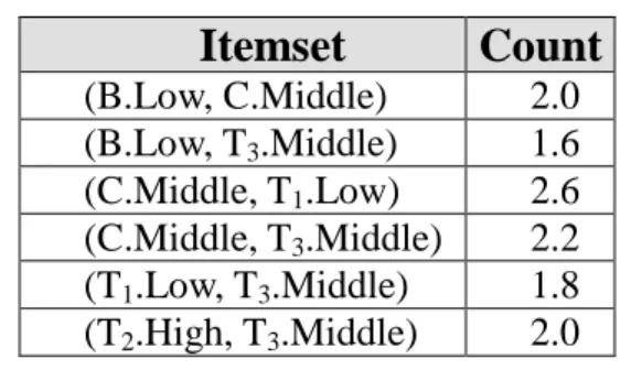
(b) The scalar cardinality (count) of each candidate 2-itemset in C2 is

Table 5.8 The fuzzy counts of the itemsets in C2

Itemset

Count

(c) Since only the count of (B.Low, T3.Middle) is smaller than the predefined

minimum support value 1.7, other two-itemset are thus kept in L2.

STEP 8: r is set at 2, where r is used to keep the number of items kept in the

current itemsets.

STEP 9: Since L2 is not null, the next step is done.

STEP 10: The candidate set C3 is generated from L2 and only the itemsets (C.Middle, T1.Low, T3.Middle) is formed.

STEP 11. The following substeps are done for each newly formed candidate

3-itemset in C3:

(a) The fuzzy membership values of each transaction data for the candidate 3-itemsets

are calculated. Here, the minimum operator is used for intersection. The results

Table8. The membership vales for C.Middle ^ T1.Low ^ T3..Middle

TID C.Middle T1.Low T3.Middl

e C.Middle∩ T1.Low∩T3.Middle T1 0.6 0.6 0.2 0.2 T2 0.8 0.6 0.8 0.6 T3 0.8 0.8 0.8 0.8 T4 0.4 0.0 0.2 0.0 T5 0.0 0.0 0.6 0.0 T6 0.6 0.8 0.2 0.2

(b) The scalar cardinality (count) of each candidate 3-itemset in C3 is calculated. Its scalar cardinality = (0.2+0.6+0.8+0.0+0.0+0.2)=1.8

(c) Since the count of (T3.Middle, T1.Low, T3.Middle) is larger than the predefined

minimum support value 1.7, it is thus kept in L3.

STEP 12: Since L3 is not null, r = r +1= 3 and STEP 10 is done again. The same

process is then executed for finding level-4 large itemsets. In this example, no level-4

large itemsets are found. STEP 13 is then executed to find the association rules.

STEP 13: The association rules are constructed for each large itemset using the

following substeps.

(a)The possible association rules for the itemsets found are formed as follows: If B = Low, then C = Middle;

If C = Middle, then B = Low; If C = Middle, then T1 = Low;

If T1 = Low, then C = Middle; If C = Middle, then T3 = Middle; If T3 = Middle, then C = Middle; If T1 = Low, then T3 = Middle; If T3 = Middle, then T1 = Low; If T2 = High, then T3 = Middle; If T3 = Middle, then T2 = High;

If C = Middle and T1 = Low then T3 = Middle; If C = Middle and T3 = Middle then T1 = Low; If T1 = Low and T3 = Middle then C = Middle.

(b)The confidence values of the above thirteen possible association rules are calculated. Take the first association rule as an example. The count of

B.Low∩C.Middle is 2.0 and the count of B.Low is 2.2. The confidence

value for the association rule "If B = Low, then C = Middle" is calculated as:

The confidence factor for the association rule "If B = Low, then C = Middle" is then:

∑

∑

If C = Middle, then B = Low has a confidence factor of 0.625; If C = Middle, then T1 = Low has a confidence factor of 0.81; If T1 = Low, then C = Middle has a confidence factor of0.93; If C = Middle, then T3 = Middle has a confidence factor of 0.69; If T3 = Middle, then C = Middle has a confidence factor of 0.79; If T1 = Low, then T3 = Middle has a confidence factor of 0.64; If T3 = Middle, then T1 = Low has a confidence factor of 0.64; If T2 = High, then T3 = Middle has a confidence factor of 0.67; If T3 = Middle, then T2 = High has a confidence factor of 0.71;

If C = Middle and T1 = Low then T3 = Middle has a confidence factor of 0.69; If C = Middle and T3 = Middle then T1 = Low has a confidence factor of 0.82; If T1 = Low and T3 = Middle then C = Middle has a confidence factor of 0.9

STEP 14: The confidence values of the possible association rules are checked

with the predefined confidence thresholdλ. Assume the given confidence thresholdλ

is set at 0.8. The six rules are following:

B.Low C.Middle [sup=2.0, conf=0.91]; C.Middle T1 .Low [sup=2.6, conf=0.81]; T1.Low C .Middle [sup=2.6, conf=0.93]; T3 .Middle C = Middle [sup=2.2, conf=0.79];

C .Middle and T3 .Middle T1 .Low [sup=1.8, conf=0.82]; T1 .Low and T3 .Middle C .Middle [sup=1.8, conf=0.9].

STEP 15: Since we consider this two rules B.Low C.Middle [sup=2.0, conf=0.91] and T1.Low C .Middle [sup=2.6, conf=0.93], "T1" is a parent of "B" with their same of linguistic term and consequent "C". The B.Low C.Middle [sup=2.0, conf=0.91] is redundant rule thus pruning in this step. The following five rules are thus output to users:

C.Middle T1 .Low [sup=2.6, conf=0.81]; T1.Low C .Middle [sup=2.6, conf=0.93]; T3 .Middle C = Middle [sup=2.2, conf=0.79];

C .Middle and T3 .Middle T1 .Low [sup=1.8, conf=0.82]; T1 .Low and T3 .Middle C .Middle [sup=1.8, conf=0.9].

7. Discussion and Conclusions

In this paper, we have proposed a fuzzy data mining generalized association rules

algorithm, which can process transaction data with quantitative values and discover

interesting patterns among them. The rules thus mined exhibit quantitative regularity

at taxonomy and can be used to provide some suggestions to appropriate supervisors.

When compared with the traditional crisp-set mining methods for quantitative

data, our approach can get smooth mining results due to the fuzzy membership

characteristics. Also, when compared with the fuzzy mining methods, which take all

between the rule completeness and the time complexity.

Although the proposed method works well in data mining for quantitative values,

it is just a beginning. There is still much work to be done in this field. In the future,

we will first extend our proposed algorithm to solve the above two problems. In

addition, our method assumes that the membership functions are known in advance.

In [17-19], we also proposed some fuzzy learning methods to automatically derive the

membership functions. Therefore, we will attempt to dynamically adjust the

membership functions in the proposed mining algorithm to avoid the bottleneck of

membership function acquisition. We will also attempt to design specific data-mining

References

[1] R. Agrawal, T. Imielinksi and A. Swami, “Mining association rules between sets

of items in large database,“ The 1993 ACM SIGMOD Conference, Washington DC,

USA, 1993.

[2] R. Agrawal, T. Imielinksi and A. Swami, “Database mining: a performance

perspective,” IEEE Transactions on Knowledge and Data Engineering, Vol. 5, No.

6, 1993, pp. 914-925.

[3] R. Agrawal, R. Srikant and Q. Vu, “Mining association rules with item

constraints,” The Third International Conference on Knowledge Discovery in

Databases and Data Mining, Newport Beach, California, August 1997.

[4] A. F. Blishun, “Fuzzy learning models in expert systems,” Fuzzy Sets and Systems,

Vol. 22, 1987, pp. 57-70.

[5] L. M. de Campos and S. Moral, “Learning rules for a fuzzy inference model,”

Fuzzy Sets and Systems, Vol. 59, 1993, pp. 247-257.

[6] R. L. P. Chang and T. Pavliddis, “Fuzzy decision tree algorithms,” IEEE

Transactions on Systems, Man and Cybernetics, Vol. 7, 1977, pp. 28-35.

[7] M. S. Chen, J. Han and P. S. Yu, “Data mining: an overview from a database

6, 1996.

[8] C. Clair, C. Liu and N. Pissinou, “Attribute weighting: a method of applying

domain knowledge in the decision tree process,” The Seventh International

Conference on Information and Knowledge Management, 1998, pp. 259-266.

[9] P. Clark and T. Niblett, “The CN2 induction algorithm,” Machine Learning, Vol. 3,

1989, pp. 261-283.

[10] M. Delgado and A. Gonzalez, “An inductive learning procedure to identify fuzzy

systems,” Fuzzy Sets and Systems, Vol. 55, 1993, pp. 121-132.

[11] A. Famili, W. M. Shen, R. Weber and E. Simoudis, "Data preprocessing and

intelligent data analysis," Intelligent Data Analysis, Vol. 1, No. 1, 1997.

[12] W. J. Frawley, G. Piatetsky-Shapiro and C. J. Matheus, “Knowledge discovery in

databases: an overview,” The AAAI Workshop on Knowledge Discovery in

Databases, 1991, pp. 1-27.

[13] T. Fukuda, Y. Morimoto, S. Morishita and T. Tokuyama, "Mining optimized

association rules for numeric attributes," The ACM SIGACT-SIGMOD-SIGART

Symposium on Principles of Database Systems, June 1996, pp. 182-191.

[14] A.Gonzalez, “A learning methodology in uncertain and imprecise environments,”

International Journal of Intelligent Systems, Vol. 10, 1995, pp. 57-371.

database,” The International Conference on Very Large Databases, 1995.

[16] T. P. Hong, C. S. Kuo and S. C. Chi, "A data mining algorithm for

transaction data with quantitative values," Intelligent Data Analysis, Vol. 3, No. 5, 1999, pp. 363-376.

[17] T. P. Hong and J. B. Chen, "Finding relevant attributes and membership functions," Fuzzy Sets and Systems, Vol.103, No. 3, 1999, pp. 389-404. [18] T. P. Hong and J. B. Chen, "Processing individual fuzzy attributes for fuzzy

rule induction," Fuzzy Sets and Systems, Vol. 112, No. 1, 2000, pp. 127-140. [19] T. P. Hong and C. Y. Lee, "Induction of fuzzy rules and membership functions

from training examples," Fuzzy Sets and Systems, Vol. 84, 1996, pp. 33-47. [20] A. Kandel, Fuzzy Expert Systems, CRC Press, Boca Raton, 1992, pp. 8-19.

[21] J. R. Quinlan, “Decision tree as probabilistic classifier,” The Fourth International

Machine Learning Workshop, Morgan Kaufmann, San Mateo, CA, 1987, pp.

31-37.

[22] J. R. Quinlan, C4.5: Programs for Machine Learning, Morgan Kaufmann, San

Mateo, CA, 1993.

[23] R. Rastogi and K. Shim, "Mining optimized association rules with categorical

and numeric attributes," The 14th IEEE International Conference on Data

[24] R. Rastogi and K. Shim, "Mining optimized support rules for numeric attributes,"

The 15th IEEE International Conference on Data Engineering, Sydney,

Australia, 1999, pp. 206-215.

[25] J. Rives, “FID3: fuzzy induction decision tree,” The First International

symposium on Uncertainty, Modeling and Analysis, 1990, pp. 457-462.

[26] R. Srikant and R. Agrawal, “Mining quantitative association rules in large

relational tables,” The 1996 ACM SIGMOD International Conference on

Management of Data, Monreal, Canada, June 1996, pp. 1-12.

[27] R. Srikant and R. Agrawal, “Mining Generalized Association Rules," The

International Conference on Very Large Databases, 1995.

[28] C. H. Wang, T. P. Hong and S. S. Tseng, “Inductive learning from fuzzy

examples,” The fifth IEEE International Conference on Fuzzy Systems, New

Orleans, 1996, pp. 13-18.

[29] C. H. Wang, J. F. Liu, T. P. Hong and S. S. Tseng, “A fuzzy inductive learning

strategy for modular rules,” Fuzzy Sets and Systems, Vol.103, No. 1, 1999, pp.

91-105.

[30] R. Weber, “Fuzzy-ID3: a class of methods for automatic knowledge acquisition,”

The Second International Conference on Fuzzy Logic and Neural Networks,

[31] Y. Yuan and M. J. Shaw, “Induction of fuzzy decision trees,” Fuzzy Sets and

Systems, 69, 1995, pp. 125-139.

[32] L. A. Zadeh, “Fuzzy sets,” Information and Control, Vol. 8, No. 3, 1965, pp.