類神經網路與基因演算法於井測資料反推

國

立

交

通

大

學

資訊學院 資訊學程

碩

士

論

文

類神經網路與基因演算法於井測資料反推

Neural Networks and Genetic Algorithms for Well

Logging Inversion

研 究 生：余勝棟

指導教授：黃國源 教授

類神經網路與基因演算法於井測資料反推

Neural Networks and Genetic Algorithms for Well

Logging Inversion

研 究 生：余勝棟 Student：Sheng-Tung Yu

指導教授：黃國源 博士 Advisor：Dr. Kou-Yuan Huang

國 立 交 通 大 學

資訊學院 資訊學程

碩 士 論 文

A Thesis

Submitted to College of Computer Science National Chiao Tung University in partial Fulfillment of the Requirements

for the Degree of Master of Science in Computer Science July 2008 Hsinchu, Taiwan

中華民國九十七年七月

類神經網路與基因演算法於井測資料反推

學生：余勝棟 指導教授

：

黃國源 博士

國 立 交 通 大 學

資 訊 學 院 資 訊 學 程 碩 士 班

摘

要

在井測資料的反推問題中，井測合成資料與地層真實導電率之間是一種非線 性的映對關係，而類神經網路能夠避免複雜的理論計算，經由訓練過程來調整權 重值，以逼近輸入輸出值之間的映對關係，因此本研究以類神經網路為基礎，發 展高階特徵值類神經網路架構，以應用於井測資料的反推。 由於常用以訓練類神經網路的梯度下降法，有易於陷入區域最小值的缺點， 因此，我們以結合基因演算法來改善網路學習的效率。另外，梯度下降法的收斂 較為緩慢，因此使用共軛梯度法來增進學習速率。為了加強網路的非線性映對能 力，我們提出高階特徵值類神經網路，其特性為使用次方函數來增加輸入特徵值 的高階項。此外，為了提高訓練樣本的數量以增進收斂效率，我們測試了不同輸 入神經元數量的網路架構。另外，經由實驗結果比較得知，含有 1 層隱藏層的網 路比不含隱藏層的網路有較好的收斂效果，因此我們採用含有 1 層隱藏層的網路。 研究資料一共是 31 口井的井測合成資料，每一口井含有 200 點的輸入與期望輸出 值資料。實驗以網路的實際輸出值與期望輸出值之間的平均絕對值誤差來評估網 路的效能，以 Leave-one-out 的方式做 31 次試驗，每次試驗用 30 組資料做訓練， 訓練完成的網路以剩下的 1 組資料做測試，經過 31 次的試驗，取其平均值做為該 次實驗的結果。 為了驗證高階特徵值類神經網路的有效性，我們以合成的資料作為輸入特徵 值來訓練網路，採用的網路架構為 30-36-10 (不含 bias)，使用共軛梯度法為訓 練法則，網路訓練完成後輸入真實的井測資料，以測試網路的反推結果。實驗顯 示，我們所提出的高階特徵值類神經網路，能夠有效的應用於井測資料的反推問 題。在以類神經網路應用於井測資料的反推問題上，我們的研究結果提供了一個 良好的網路架構。 關鍵字:類神經網路，基因演算法，井測資料反推。

Neural Networks and Genetic Algorithms for Well Logging

Inversion

Student：Sheng-Tung Yu

Advisor：Dr. Kou-Yuan Huang

Degree Program of Computer Science

National Chiao Tung University

ABSTRACT

In well logging inversion problem, a non-linear mapping exists between the synthetic logging measurements and the true formation conductivity. Without complexity of theoretic computation, neural network is able to approximate the input-output mapping through training with the iterative adjustment of connection weights. In our study, we develop the higher-order feature neural nets on the basis of neural network, and then apply on well logging inversion.

The usually used training algorithm for neural network is gradient descent, which is easy to get trapped at local minimum, so we adopt a method that combine with genetic algorithm to improve the training efficiency. In addition, the convergence of gradient descent is slow, so we adopt the conjugate gradient to speed up the convergence. In order to make network more non-linear, we proposed higher-order feature neural nets that use functions to expand the input feature to higher degree. In order to use more training patterns and increase the convergence efficiency, we test various network architectures that use different number of input nodes. Besides, the experimental results show that the convergence efficiency of the network with 1 hidden layer is better than that without hidden layer, so we adopt the network with 1 hidden layer. We use 31 synthetic logging datasets. Each has 200 input features and corresponding outputs. The performance of network is evaluated by comparing the mean absolute error between the actual outputs and desired outputs. Leave-one-out validation method is used in experiments. Each time 30 datasets are used in training, the trained network is then tested with the left 1 dataset. After 31 trials, the network performance is computed by averaging these testing results.

To validate the effectiveness of higher-order feature neural nets, the network size is 30-36-10 (not include bias), we train the network using conjugate gradient with synthetic logging datasets, and the trained network is then tested with real field logs. Results obtained from our experiments have shown that the proposed higher-order feature neural nets can be used effectively to process the well logging inversion. Our study shows an effective architecture of neural network to apply on well logging data inversion.

誌

謝

感謝恩師黃國源博士，ㄧ年多以來不厭其煩地給予學生指導，使學生不僅在 學業上得到許多啟發，對於老師治學的嚴謹態度與做研究實事求是的精神，更是 學生不管在求學上與工作上所積極學習的典範，令我受益良多。 感謝劉長遠教授、王榮華教授、以及蘇豐文教授，在口試期間給予學生修改 論文上的諸多寶貴建議。 感謝實驗室的同學們，在這一段時間以來所給予我的鼓勵與幫助。最後感謝 家人朋友以及所有關心我的人，謝謝你們陪我一路走來。

Contents

摘要

………

…

………

i

Abstract

………

…

………

ii

誌謝

………

…

………

iii

Contents

………

…

………

iv

List of Tables ………

…

………

v

List of Figures ………

…

………

vi

1

Introduction ………

…

………

1

2 Training

Neural

Network with Gradient Descent

Method ………

4

2.1 Multilayer Perceptron ………

4

2.2 Gradient Descent Method ………

5

2.3 Momentum Term ………

₆

3

Training Neural Network with Conjugate Gradient

Method ………

₇

3.1 _{Conjugate Gradient Method}

_………

₇

3.1.1 Conjugate Directions ………

8

3.1.2 Quadratic Termination of Conjugate Gradient Method …………

11

3.1.3 Construction of Conjugate Directions ………

₁₄

3.2 Back-Propagation with Conjugate Gradient Method ………

₂₅

3.2.1 Golden Section Search ………

₂₇

3.2.2 Training Process Using Conjugate Gradient Method ………

₃₅

4

Experiments on Well Logging Inversion ………

40

4.1 Data Pre-processing ………

41

4.2 Determination of the Stopping Error ………

₄₁

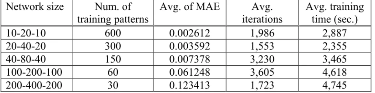
4.3 Determination of the Number of Input Nodes ………

₄₂

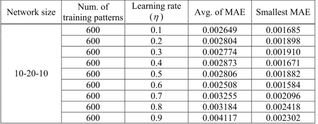
4.4 Determination of the MLP Network Parameters ………

₄₅

4.5 Higher-Order Feature Multi-Layer Neural Net (HOML) ………

₅₀

4.6 Higher-Order Feature Multi-Layer Neural Net with Conjugate Gradient ( HOCG ) ………

56

4.7 Experiments on Reversing Input and Output of Well Logging Data ………

59

4.8 Summary ………

62

5

Genetic Algorithm (GA) on Well Logging Inversion…

64

5.1 Introduction ………

₆₀

5.2 Real-Coded Genetic Algorithm (RCGA) ………

₆₇

5.3 Experiments on Well Logging Data Inversion ………

₆₈

5.3.1 Representation of Weights of Neural Network ………

₆₈

5.3.2 Combination of Neural Network and GA ………

69

5.3.3 Evaluation of Hybrid Neural Network and GA ………

70

5.3.4 Experiments on Reversing the Input and Output of Well Logging Data ………

72

5.3.5 Summary ………

74

6

Experiments on Real Field Logs ………

76

7

Conclusions ………

80

List of Tables

Table 3-1 Result of conjugate gradient for 2 iterations ……… 21

Table 3-2 Result of gradient descent for 6 iterations ……… 22

Table 3-3 Computation process of interval location ……… 29

Table 3-4 Computation process of Golden Section Search ……… 35

Table 4-1 The network performance using different stopping errors ………… 42

Table 4-2 Experimental result of each kind of MLP network ……… 44

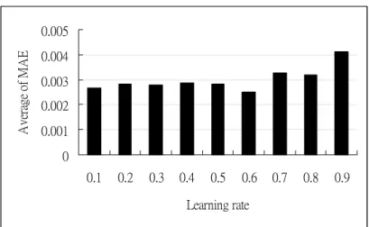
Table 4-3 MLP network performance with different learning rate ……… 45

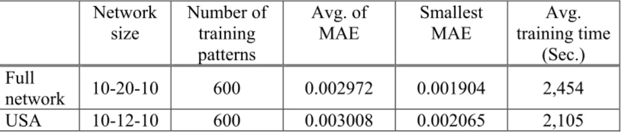
Table 4-4 Number of hidden nodes by USA algorithm ……… 49

Table 4-5 Comparison of MLP network performance between full network and the network that pruned by USA algorithm ……… 49

Table 4-6 Comparison of MLP network performance with one and two hidden layers ……… 50

Table 4-7 Five different HOML types ……… 51

Table 4-8 Five different HOSL types ……… 52

Table 4-9 Testing results of HOSL and HOML ……… 53

Table 4-10 Testing result of each type of HOML ……… 55

Table 4-11 Five different HOCG types ……… 57

Table 4-12 Comparison of each types of HOCG ……… 57

Table 4-13 Comparison of average of mean absolute error between HOML and HOCG ……… 57

Table 4-14 Average of mean absolute error with 10, 20, 40, and 50 input nodes in HOML-1 ……… 60

Table 4-15 Average of mean absolute error of HOML and HOCG ………… 61

Table 4-16 Training time of HOML and HOCG in seconds ……… 61

Table 4-17 Comparison of HOML and HOCG in average of mean absolute error and average training time ……… 63

Table 4-18 Comparison of experimental results of reversing the input and output of well logging data ……… 63

Table 5-1 Testing results of HOML with GA ……… 71

Table 5-2 Average performance of three hybrid methods ……… 73

Table 5-3 Comparison of HOML and HOCG in average of mean absolute error and average training time ……… 75

Table 5-4 Comparison of experimental results of reversing the input and output of well logging data ……… 75

List of Figures

Fig. 1-1 Experiments flowchart ……… 3

Fig. 2-1 MLP network with one hidden layer ……… 5

Fig. 3-1 The iterative computation ……… 8

Fig. 3-2 Graph of a quadratic form ……… 9

Fig. 3-3 Conjugate gradient method finds minimum in 2 iterations ………… 11

Fig. 3-4 Conjugate gradient method converges in n iterations ……… 12

Fig. 3-5 Gram-Schmidt conjugate process ……… 15

Fig. 3-6 Conjugate gradient method with exact step ……… 21

Fig. 3-7 Gradient descent method with exact step ……… 22

Fig. 3-8 The curve in (a) gradient descent and (b) conjugate gradient when step size is 0.1 ……… ₂₃

Fig. 3-9 The curve in (a) gradient descent and (b) conjugate gradient when step size is 0.4 ……… ₂₄

Fig. 3-10 MLP network ……… 25

Fig. 3-11 Interval location ……… 27

Fig. 3-12 Result of interval location ……… 29

Fig. 3-13 Minimum occurs in interval [x1, xc] ……… 30

Fig. 3-14 Minimum occurs in interval [xa, x2] ……… 30

Fig. 3-15 Two initial internal points ……… 31

Fig. 3-16 Interval reduction ……… 32

Fig. 3-17 Flowchart of Golden Section Search ……… 34

Fig. 3-18 Flowchart of conjugate gradient back-propagation algorithm to train MLP network ……… 39

Fig. 4-1 Three samples of well logging datasets ……… 41

Fig. 4-2 Testing result of MLP network with 200 input nodes ……… ₄₃

Fig. 4-3 MLP network with smaller number of input nodes ……… 44

Fig. 4-4 Average performance with different number of input nodes ……… 45

Fig. 4-5 Mean absolute error in MLP networks with different learning rate … 46 Fig. 4-6 The MLP network ……… 47

Fig. 4-7 Flowchart of USA algorithm ……… 49

Fig. 4-8 HOML-2 with original and expanded features ……… 51

Fig. 4-9 HOSL-2 with original and expanded features ……… 53

Fig. 4-10 Comparison of MSE curve between HOML-5 and HOSL-5……… 54

Fig. 4-11 Average of mean absolute error in different HOML networks …… 55

Fig. 4-12 Testing result of HOML-5 on dataset number 23 ……… 55

Fig. 4-13 Training time for each dataset in 5 HOML networks ……… 56

Fig. 4-14 Testing case of HOCG-5 on dataset number 10 that does not achieve the training goal ……… 58

Fig. 4-15 Testing case of HOCG-5 on dataset number 10 that achieves the training goal ……… 58

Fig. 4-16 Testing case of HOCG-2 on dataset number 12 ……… 59

Fig. 4-18 Comparison of network performance in HOML and HOCG …… 62

Fig. 5-1 Binary format of an individual with 3 genes ……… 64

Fig. 5-2 Single point crossover from two individuals, each element of individual is a gene ……… 65

Fig. 5-3 Flowchart of genetic algorithm ……… 65

Fig. 5-4 Arithmetic crossover ……… 67

Fig. 5-5 A MLP network represented by an individual ……… 68

Fig. 5-6 Flowchart of the hybrid method on well logging inversion ………… 70

Fig. 5-7 Testing results in HOML-2 with GA and HOML-3 with GA …… 72

Fig. 5-8 Testing results of HOML with GA ……… 74

Fig. 6-1 Two samples of MSE curve while in training ……… 76

Fig. 6-2 The inverted true formation resistivity between 5,577.5 to 5,827 feet 77

Fig. 6-3 The inverted true formation resistivity between 5,827.5 to 6,077 feet 77

Fig. 6-4 The inverted true formation resistivity between 6,077.5 to 6,327 feet 77

Fig. 6-5 The inverted true formation resistivity between 6,327.5 to 6,682 feet 78

1. Introduction

Multilayer perceptron (MLP) network consists of one or more hidden layers between the input layer and the output layer. Since the back-propagation (BP) learning algorithm that was developed by Rumelhart, Hinton, and Williams in 1986, MLP network has been successfully used on a wide range of applications [1]. The BP learning algorithm uses gradient descent method that calculates the negative gradient of the error with respect to the weights for a given input. The gradient descent method has some drawbacks [2]. For example, it takes long time in training. To speed up the training process, some optimization algorithms, such as conjugate gradient method, are employed to train MLP network. Martin et al. [3] developed a method that utilizes neural network to process the well logging data. Their results showed that the network trained by conjugate gradient was more effective in the well logging inversion than the other existing methods. Their new approach first train the network with conjugate gradient method and later switch to the LM algorithm, to refine the network parameters. In this paper, we use conjugate gradient to train the network, also we expand the features to higher degree.

Another drawback of gradient descent is easy to get trapped at the local minimum. On the other hand, genetic algorithm is a global search algorithm that is inspired by evolution. An implementation of genetic algorithm starts from an initial population that consists of chromosomes. A chromosome is called an individual that is a candidate solution to the target problem. Fitness value of individual is computed through fitness function during evolution. The individual with higher fitness value has more chance to survive and generates offspring in next generation and finally converges to a global minimum. However, since genetic algorithm is usually slow, some researches and applications that combined genetic algorithms and other algorithms were studied. Tan [4] combined genetic algorithm and evolutionary programming which always applies the mutation operator on bias and weights in iteration to train a neural network, and applied on the cancer classification problem. Kinnebrock [5] designed a hybrid method that combines genetic algorithm and neural network. The author demonstrated that the iterative number in training neural network could be reduced, if after iteration the weights are changed by a mutation

[6] that combines genetic algorithm and neural network to apply on the well logging data inversion problem. The idea is to refine the connection weight using BP learning with gradient descent after every generation.

The remaining of this paper is as follows. Chapter 2 gives an overview of MLP network, the BP learning algorithm with gradient descent. Chapter 3 describes the conjugate gradient method and the BP learning algorithm with conjugate gradient method. Chapter 4 describes the experiments on well logging data inversion. For the network architecture, we test the different learning rate, the number of hidden nodes, and the number of hidden layers. We design 5 higher-order feature neural nets, which expand the input features to higher degree, to apply on the experiments of well logging data inversion. Comparison of these nets that trained by gradient descent and conjugate gradient will be made. Chapter 5 describes the genetic algorithm, the real-coded genetic algorithm, and the used hybrid method that combines the neural network and genetic algorithm on the experiments of well logging data inversion. Chapter 6 and Chapter 7 give the experiments on real field logs and conclusions. Figure 1-1 is the flowchart of the experiments in our study.

2. Training Neural Network with Gradient

Descent Method

2.1 Multilayer Perceptron

A MLP network consists of a set of nodes that are fully connected and are organized into multiple layers. Typically MLP network has three or more layers of nodes: an input layer that accepts input data, one or more hidden layers, and an output layer. There are bias parameters in input layer and hidden layer that act as extra nodes with a constant output value of 1. For arbitrary node j, the weighted sum of inputs is: ( 1) 1 d j i ji j i net x w w d+ = =

∑

+ (2-1)

where d is the number of input data to the node, xi is an input, wji is the connection

weight between node i and j, and wj(d+1) is the connection weight corresponding to

the bias parameter. The output of node j is f(netj) where f is the activation function.

MLP network usually use differentiable sigmoidal activation function for hidden and output nodes [7]. The formula of sigmoidal function is as follows.

-1 ( ) 1 net f net e = + (2-2) ( )

f net′ = f net( )(1− f net( )) (2-3)

MLP network is trained by supervised learning. Supervised learning requires a desired response to be trained, and is based on the comparison between the actual output of network and the desired output. The learning process of MLP network has two phases, one is the forward computation and the other is the backward learning [8]. In forward computation, training pattern is presented to the network from the input layer, and transmit to the hidden layers, the outputs of hidden layers are then transmitted to output layer, finally the real output values are computed. In backward learning phase, the error between the real output value and the desired output value is propagated back to the network to update the connection weights. Figure 2-1 is the example of MLP network with one hidden layer.

. . . . . . . . .

x

1

y

1

x

2

x

i

y

2

y

k

Input layer Output layer

Weight wji between input layer and hidden layer

Weight wkj between hidden layer and output layer

1

1

h

j

h

1

h

2

h

3 Hidden layer

Fig. 2-1. MLP network with one hidden layer.

2.2 Gradient Descent Method

Gradient descent method is a function optimization method that uses the negative derivative of the function. MLP network is often trained using the gradient descent method. Assuming we have a MLP network with one hidden layer. There are I nodes in input layer (not including the bias), J nodes in hidden layer (not

including the bias), and K nodes in output layer, i, j, and k denote the node index. wkj

denotes the weight value connecting output node and hidden node, and wji denotes

the weight value connecting hidden node and input node. The BP algorithm is to modify the weight value iteratively so that the error function of network E is minimized. An error function of a network E is defined as follows.

2 1 1 E ( 2 K k k k d y = =

∑

− ) (2-4)

where dk and yk denote the desired output value and the real output value of the kth

outputnode respectively.

According to the gradient descent method, the weight change is in the reverse direction of the gradient. The formula of weight change in hidden node and output node is:

( 1) ( ) kj kj kj kj E w w t w t w η ∂ Δ = + − = − ∂ (2–5)

where η is the learning rate and t is the iteration index.

By applying the chain rule on equation (2-5), the weight change in hidden node and output node is:

( ) ( )

kj k k k j

w η d y f net′

Δ = − y (2-6)

Similarly, the weight change in input node and hidden node is:

( 1) ( ) ji ji ji ji E w w t w t w η ∂ Δ = + − = − ∂ (2-7)

By applying the chain rule on equation (2-7), the weight change in input node and hidden node is:

1 [ K ( ) ' ( ) ] ' ( ) ji k k k kj k w

η

d y f net w f net = Δ =

∑

− _j y_i (2-8)

2.3 Momentum Term

In equation (2-5) and (2-7), the learning rate determines the speed of convergence by acting as a step size. If it is too large, the network training may fail to convergence because of oscillation. On the other hand, smaller learning rate may get slow convergence in training. To get the advantage of using large learning rate and to lessen the oscillation, Rumelhart et al. (1986) [9] suggested adding a momentum term to stabilize the weight change. The weight update at a given iteration index t becomes:

( )

(

) ' (

)

( 1)

kj k k k j kj

w t

η

d

y f

net y

β

w t

Δ

=

−

+ Δ

−

between hidden and

output node, and

1

( )

[

K

(

) ' (

)

] ' (

)

(

1)

ji k k k kj j i ji k

w t

η

d

y f

net w f

net y

β

w t

=

Δ

=

∑

−

+ Δ

−

3. Training Neural Network with Conjugate

Gradient Method

3.1 Conjugate Gradient Method

The gradient descent method simply uses the first order (gradient) information, however, using the second order information is often more effective in convergence [10]. There has been technique about the usage of second order information, such as Newton’s method [2]. The Newton’s method requires storage and expensive computation cost of the inverse Hessian matrix. On the other hand, the conjugate gradient method takes advantages of the second order information but not requires the process of the Hessian matrix [11]. The major difference between the gradient descent method and the conjugate gradient method is in finding the search direction. In gradient descent method, the search direction is always the negative of gradient; however, in conjugate gradient method the search direction is the conjugate direction to improve the search efficiency [12]. 本研究使用 Matlab v7.1 的類神經

網路 Toolbox，以共軛梯度法來訓練類神經網路，並應用於井測資料的反推。 有關於共軛梯度演算法以及一維線性搜尋法(黃金分割法)，將分別於後面的章 節中描述。 共軛梯度法的步驟，是在某一搜尋點 x(i)處選擇一個新的搜尋方向 d(i)， 使其與前次的搜尋方向 d(i-1)滿足 A-共軛 [2]，即： d(i)TAd(i-1) = 0 (3-1) 然後從搜尋點 x(i)處出發，沿著搜尋方向 d(i)，求得函數 f(x)的極小點所需

的步長α(i)，亦即求得 α(i)使得 f(x(i) + α(i)d(i))具有最小值。經由所找到的搜尋

方向 d(i)與步長 α(i)，可以依照疊代式算法計算出下一搜尋點 x(i+1)，即由公式 (3-2)以及圖(3-1)所示：

x(i+1) = x(i) + α(i)d(i) (3-2)

圖(3-1)顯示由起始點 x(0)出發，沿著所選定的方向 d(0)移動 α(0)距離後，可以 計算出新的搜尋點 x(1)，再由點 x(1)開始，決定所需的方向 d(1)與步長 α(1)， 計算新的搜尋點，依此計算方式一步步逼近問題解。

Fig. 3-1. The iterative computation. 接下來的章節，將針對二次函數探討共軛梯度法的性質，3.1.1 節將說明共 軛方向，對於求函數極小點問題時，比使用負梯度方向有較好的效率；3.1.2 節 說明共軛梯度法的二次終結性(Quadratic Termination)，也就是對於 n 維度的二 次函數，在n 次 iteration 內就能到達極小點；在探討了共軛方向的性質後，3.1.3 節將說明在共軛梯度法中，求得共軛方向的方法。

3.1.1 Conjugate Directions

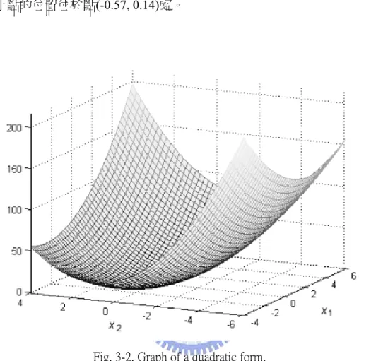
本小節說明在二次函數的求極值問題上，在任一搜尋點決定下一個要搜尋 的方向時，如果以共軛方向當成搜尋方向，會比梯度下降法使用負梯度的搜尋 方向更有效率。 對於一個二次函式有以下的一般表示式 [2]： T T 1 ( ) 2 f x = x Ax +b x+c (3-3) 其中 A 為對稱正定矩陣，而梯度 [2] 則為： ▽f(x) = Ax + b (3-4)

方程組 Ax + b = 0 的解則為此二次函數的極小點。圖(3-2)所示為二次函數 T T 1 ( ) 2 f x = x Ax +b x+c的3D 曲線圖，其中 A= 4 2 2 8 ⎡ ⎤ ⎢ ⎥ ⎣ ⎦，b= 2 0 ⎡ ⎤ ⎢ ⎥ ⎣ ⎦，以及c = 0， 其最小點的位置位於點(-0.57, 0.14)處。

Fig. 3-2. Graph of a quadratic form.

以下的敘述開始說明共軛方向的特性(Jonathan Richard Shewchuk，[12])， 為了方便說明, 以符號 r(i) 表示在第 i 步時，Ax 與 Ax(i) 之間的差異：

r(i) = Ax – Ax(i) r(i) = –b – Ax(i) r(i) = –▽f(x(i)) _(3-5) 另外，以誤差向量Δx(i)，表示真實解與估計值之間的差異： Δx(i) = x - x(i) (3-6) 關於誤差向量Δx 與方向 d 的關係式，可經由公式(3-2)與(3-6)得出：

x(i+1) = x(i) + α(i)d(i)

x – x(i+1) = x – x(i) – α(i)d(i)

數 f(x( ) +i α( ) ( ))i d i 能夠極小化，可以令 f(x( ) +i α( ) ( ))i d i 對 α(i)的導數為零， 也就是： ( ( ) ( )) ( ) d f i i i d iα x( ) +α d = 0 ( +1 ) 0 ( ) d f i d iα x( ) = f’(x(i+1))T +1 ( ) d i d iα x( ) = 0 -rT(i+1)d(i) = 0

(Ax(i+1)–Ax)Td(i) = 0 (by equation (3-5))

A(x(i+1)–x)Td(i) = 0

–A x(i+1)Δ T

d(i) = 0

d(i)TAΔx(i+1) = 0 (3-8)

根據公式(3-1)關於 A-共軛的定義，得出 d(i)與Δx(i+1)是兩個滿足 A-共軛

的方向；繼續整理公式(3-8)以求得步長 α(i)：

d(i)TA(Δx(i) – α(i)d(i)) = 0 (by equation (3-7)) d(i)TAΔx(i) – d(i)TAα(i)d(i) = 0

α(i) = T T ( ) ( ) ( ) ( ) i i i i Δ d A x d Ad = T T ( ) ( ) ( ) ( ) i i i i − d r d Ad α(i) = T T ( ) ( ( )) ( ) ( ) i f i i i −d ∇ x d Ad (3-9) 此處的方向 d(i)若是以 r(i)來取代，則公式(3-9)即相當於梯度下降法中計算 步長的公式，亦即： α(i) = T T ( ) ( ) ( ) ( ) i i i i r r r Ar α(i) = T T )) )) )) )) f i f i f i f i ∇ ∇ ∇ ∇ (x( (x(

(x( A (x( , for gradient descent method. (3-10)

如圖(3-3)與公式(3-8)所示，從起始點 x(0)沿著方向 d(0)移動，找到最佳步

梯度法選擇 x(1)當成是下一個方向 d(1)，那麼在求解二維的二次方程式問題 時， 兩步之內即可找到極小點，比起使用負梯度的搜尋方向(r(1))更有效率。

Δ

Fig. 3-3. Conjugate gradient method finds minimum in 2 iterations.

3.1.2 Quadratic Termination of Conjugate Gradient

Method

上一小節說明，在一個二維的二次函數中，共軛梯度法僅需兩步即能到達 極小點，本小節則進一步說明共軛梯度法的二次終結性，亦即在一個n 維度的 二次函數中，在最多n 次疊代之後就能找到極小點 [2]。也就是經過 n 次疊代 之後: Δx(n) = 0 以 下 的 敘 述 開 始 說 明 共 軛 梯 度 法 的 二 次 終 結 性(Jonathan Richard Shewchuk，[12])，如圖(3-4)所示，起始的誤差向量(虛線部份)Δx(0)是由兩個 滿足 A-共軛的向量 d(0)與 x(1)線性組合而成，對 n 維的二次函數而言，由於 搜尋方向集合{d(i)}滿足 A-共軛，因此誤差向量 Δ Δx(0)可以表示成搜尋方向 d(i)

的線性組合： 1 0 (0) n ( ) ( ) i i i − = Δx = δ

∑

d (3-11) 以δ(i)代表集合中任一搜尋方向 d(i)的係數。

Fig. 3-4. Conjugate gradient method converges in n iterations.

為了計算出δ(i)的值，在此先利用公式(3-7)得出Δx(i)的關係式，也就是：

Δx(i+1) = Δx(i) – α(i)d(i) (公式(3-7))

將此公式中i 的數值由 0 代到 i, 得出以下方程組:

Δx(1) = Δx(0) – α(0)d(0)

Δx(2) = Δx(1) – α(1)d(1)

Δx(3) = Δx(2) – α(2)d(2)

…

Δx(i) = Δx(i–1) – α(i–1)d(i–1)

1 0 ( ) i ( ) j i − j = Δx = Δ (0) −x

∑

α( )d j _(3-12) 利用公式(3-12)有關 x(i)的關係式，即可開始計算Δ δ(i)的值。由於搜尋方 向d(i)滿足A-共軛的性質，因此可以利用將公式(3-11)兩邊各乘以d(k)TA的方 法，消除大部分的δ(i)項，最後只會留下一個，其中k介於 0 與n-1： 1 0 (0) n ( ) ( ) i i i − = Δx = δ

∑

d (公式(3-11)) 1 T T 0 T T T T T T (0) ) ( ) (0) (0) (0) (1) (1) ... ( ) ( ) (0) ) ( n i k i k i k k k i k i k k k − = Δ = δ( Δ = δ + δ + δ Δ = δ(

∑

d( ) A x d( ) Ad d( ) A x d( ) Ad d( ) Ad d( ) Ad d( ) A x d( ) Ad T T 1 T 0 T

) (by -conjugate property)

( ) (0) ) = ( ) ( ) ( ) ( (0) ( ) ( )) by -conjugate property of ( ) ( ) k j k k k k k k j j k k − = Δ δ( Δ − α =

∑

( A d A x d Ad d A x d A d Ad 1 T 0 k ( ) ( ) ( )=0) j j k j − = α

∑

d Ad T 1 T 0 ( ) ( ) ) = (by ( ) ( )) ( ) ( ) k j k k k k k k − = Δ δ( d A x Δx = Δ (0) −x

∑

α( )d d Ad j j (3-13) 由公式(3-9)與(3-13)，可以整理出α(i)與δ(i)的關係如下： T T T T T T ( ) ( ( )) ( ) ( ) ( ) ( ) ( ) ( ) ( ) ( ) ( ) ( ) ( ) ( ) i f i i i i i i i i i i i i i ∇ α = − = Δ = = δ d x d Ad d r d Ad d A x d Ad ( )i ( )i α = δ _(3-14)

現在可以將公式(3-12)關於Δx(i)的關係式做以下的改寫： 1 0 1 1 0 0 ( ) (0) ( ) ( ) = ( ) ( ) ( ) ( ) i j n i j j i j j j j j − = − − = = Δ = Δ − α δ − δ

∑

∑

∑

x x d d d j j 1 =i ( ) n ( ) ( ) j i − j Δx = δ

∑

d (3-15)

上式的意義表明，在第i step 時的誤差向量Δx(i)，等於從第 i 到第 n-1 step

之間的項目總和，也就是說每經過一次疊代，就會有一個項目被消除掉，因此， 經過n 次疊代之後，Δx(n) = 0，由此得知，在 n 維的二次函數中，最多經過 n 次的疊代即能到達極小點。 以下為n = 3 的實例說明： (0) (0) (0) + (1) (1) + (2) (2) Δx = δ d δ d δ d d (1) (1) (1) + (2) (2) Δx = δ d δ (2) (2) (2) Δx = δ d (3) 0 Δx = 每一次 iteration 之後，都會減少一項δ與 d的乘積項，經過 3 次 iteration 後， 得到誤差向量Δx(3) 0= ，也就是已到達極小點。

3.1.3 Construction of Conjugate Directions

由 3.1.1 與 3.1.2 小節可以得知，採用共軛方向當成每一次疊代的搜尋方

向，能夠有比較好的搜尋效能。因此，本小節即介紹求得一組共軛方向 d(0)，

d(1)，…，d(n-1)的方法 (Jonathan Richard Shewchuk，[12])，其中 n 代表二次

函數的維度。

求得共軛方向的過程稱為Gram-Schmidt Conjugate Process [12]。 假設空間 中有n 個獨立的向量u(0)，u(1)，…，u(n-1)，要建立i>0 的任一方向d(i)，可以

取u(i)減去它的其中一個未滿足與前方向A-共軛的分量。如圖(3-5)所示，從兩

個獨立的向量u(0)與u(1)開始，令d(0) = u(0)，而u(1)是由兩個分量u*與u+組合

而成，其中u*與前一次方向d(0)滿足A-共軛，而u+則是與d(0)平行的分量，也

d(1)，在Gram-Schmidt正交化過程中, 投影可以用內積乘上d(0)來表示，在此則

以係數β(1, 0)表示：

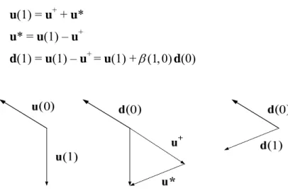
u(1) = u+ + u* u* = u(1) – u+

d(1) = u(1) – u+ = u(1) +β(1, 0)d(0)

Fig 3-5. Gram-Schmidt conjugate process.

同理，d(2)等於 u(2)減去在 d(0)的投影以及在 d(1)的投影，也就是： d(2) = u(2) +β(2, 0)d(0) +β(2,1)d(1) 因此，對於任意搜尋方向 d(i)可以表示成： 1 0 ( ) ( ) i ( , ) ( ), > k i i − β i k k i = = +

∑

d u d k (3-16) 為了計算β( , )i k 的值，將上述公式(3-16)乘上d(j)TA，其中i > j： 1 T T T 0 T T T T T ( ) ( ) ( ) ( ) ( , ) ( ) ( ) 0 = ( ) ( ) + ( ,0) (0) ( )+ ( ,1) (1) ( )+ ... + ( , ) ( ) ( ) 0 = ( ) ( ) + ( , ) ( ) ( ), > (by -conjugate property) i k i j i j i k k j i j i j i j i k k i j i j j j i j β β β β β − = = +

∑

d Ad u Ad d Ad u Ad d Ad d Ad d Ad u Ad d Ad A T j T T ( ) ( ) ( , ) = ( ) ( ) i i j j j β −u Ad d Ad j , i > j (3-17)

如公式(3-16)所示，Gram-Schmidt Conjugate Process 的缺點在於，在建立一個 新的搜尋方向 d(i)時，之前的 i-1 次方向都必須保留下來，一個改善的方法是， 使用 r(i)來取代之前使用的 u(i) [12]，也就是說，令 u(i) = r(i)，因此，計算搜 尋方向的公式(3-16)可以改寫成公式(3-18)的形式，公式(3-17)也可以改寫成公

式(3-19)。 1 0 ( ) ( ) i ( , ) ( ), > k i i − β i k k i = = +

∑

d r d k (3-18) T T ( ) ( ) ( , ) = ( ) ( ) i i j j j β −r Ad d Ad j , i > j (3-19) 為了求出d(k)與r(i)的關係(其中 i > k)，將公式(3-15)乘上d(k)TA： 1 =i 1 T T = T T T ( ) ( ) ( ) ( (3-15)) ( ) ( ) ( ) ( ) ( ) = 0 ( ( )) = 0 ( ( )) = 0 n j n j i i j j k i j j k k i k i k i − − Δ = δ Δ = δ Δ − −

∑

∑

x d d( ) A x d Ad d( ) A x d( ) A x x d( ) Ax Ax 公式 T

( ) ( ) = 0, > (by -conjugate property)k i i k

d r A _(3-20) 由上式(3-20)得知，r(i)與舊的搜尋方向 d(k)之間成正交的關係。 接下來說明，在任一點 x(i)上建立新搜尋方向 d(i)的方法，在過程中也會 說明在使用 r(i)取代 u(i)的情況下，則可以不用保留所有舊方向，僅利用前一次 的方向 d(i-1)，即可建立新方向 d(i)。 首先，利用公式(3-18)，在式子的兩邊分別取與項目 r(j)的內積，其中 j i≠ ： 1 0 ( ) ( ) ( , ) ( ), > i k i i − β i k k i = = +

∑

d r d k (公式(3-18)) 1 T T T 0 ( ) ( ) ( ) ( ) i ( , ) ( ) ( ) k i j i j − β i k k j = = +

∑

d r r r d r T T 0 ( ) ( ) (by equation ( ) ( ) 0)i j i j = r r d r = _(3-21) 另外可得： T T ( ) ( ) = ( ) ( )d i r i r i r i (3-22) 另外，由公式(3-20)的推導過程中，可以得出 r(i)與Δx(i)的關係式，也就 是 r(i) = A x(i)，因此： Δ

r(i+1) = AΔx(i+1)

r(i+1) = A(Δx(i) – α(i)d(i)) (由公式(3-7)) r(i+1) = AΔx(i) – Aα(i)d(i)

r(i+1) = r(i) – α(i)Ad(i) (3-23)

接下來，為了求出β( , )i j 的值，將上述公式(3-23)以 j 來取代 i，並且與項 目 r(i)做內積，這樣做的原因是要求得 ，以便應用於公式(3-19)中求 得 T ( )i ( ) r Ad j ( , )i j β 的值： r(j+1) = r(j) – α(j)Ad(j)

r(i)Tr(j+1) = r(i)Tr(j) – α(j) r(i)TAd(j)

α(j) r(i)TAd(j) = r(i)Tr(j) – r(i)Tr(j+1)

T 1 T ( ) ( ) = ( ) ( ) ( ) ( +1)) ( ) i j i j i j j − α r Ad (r r r Tr 從以下三種狀況來考慮r(i)TAd(j)項: T T T T T 1 (a) ( ) ( ) = ( ) ( ), = ( ) 1 (b) ( ) ( ) = ( ) ( ), = +1 ( -1) (c) ( ) ( ) 0, > +1 i j i i i j i i j i i i j i i j i j α − α = r Ad r r r Ad r r r Ad 在此忽略上述的狀況(a)，因為當 i = j 的時候，計算β( , )i j 無意義，因此， 依上述狀況(b)與狀況(c)分別將β( , )i j 重新寫成： T T T T ( ) ( ) 1 ( ) ( ) (1) ( , ) = = +1 ( ) ( ) ( 1) ( -1) ( -1) i j i i i j i j j j i i i β − = , α − r Ad r r d Ad d Ad _(3-24) T T ( ) ( ) (2) ( , ) = 0, > +1 ( ) ( ) i j i j i j j j β −r Ad = d Ad _(3-25) 由於 1 ，並且如公式(3-25)所示， 0 ( ) ( ) i ( , ) ( ) j i i − β i j j = = +

∑

d r d β( , ) = 0 if > +1i j i j , 因此得知，欲求得方向 d(i)，不再需要第 i-1 步之前的所有舊方向，只要知道 ( , )i j β 的值(其中 j = i-1)，即可藉由前一次的方向 d(i-1)求得。由此，改寫

( , ) = ( ,( -1)) = ( )i j i i i

β

β

β

。經過以上的討論，可以整理出當i>0 時，任一點 x(i) 的搜尋方向 d(i)的計算公式： T T T T T T ( ) ( ) ( , ) ( ) = ( ) + ( ) ( -1), > 0 ( ) ( ) ( ) ( (3 24) (3 9)) ( -1) ( -1) ( ) ( ) ( ( -1) ( -1) = ( -1) ( -1)) ( -1) ( -1) i i i j j i i i i i i i i i i i i i i i i i β β β = + = − − = d r d r d r r d r r r d r r r r r 其中 由公式 與 由

由於 r(i) = –▽f(x(i))，因此可以將計算搜尋方向 d(i)的公式整理如下：

(0)= − ∇f( (0)) d x ( )i = − ∇f( ( ))i +β( ) ( -1)i i d x d , i > 0 其中 T T ( ( )) ( ( )) ( ) ( ( -1)) ( ( -1)) f i f i i f i f i β = ∇ ∇ ∇ ∇ x x x x 以下針對二次函數求極小值的問題，以共軛梯度法求解的過程，寫成演算 法的形式：

Algorithm 3-1: To minimize quadratic function using conjugate gradient method. Input: Start point x(0).

Output: The solution x.

Step1: 設 iteration index i = 0 計算搜尋點 x(0)處的梯度▽f(x(0))，並且將第一次的搜尋方向設為負梯度 方向： d(0) = –▽f(x(0)) 計算步長 α(0) = T T (0) ( (0)) (0) (0) f −d ∇ x d Ad 更新到搜尋點 x(1) = x(0) +α(0)d(0)

Step2: 設 i = i + 1 計算搜尋點 x(i)處的梯度▽f(x(i)) 計算係數β(i)： T T ( ( )) ( ( )) ( ) ( ( -1)) ( ( -1)) f i f i i f i f i β = ∇ ∇ ∇ ∇ x x x x 計算新的搜尋方向 d(i)： ( )i = − ∇f( ( ))i +β( ) ( -1) i i d x d 計算步長α(i)： α(i) = T T ( ) ( ( )) ( ) ( ) i f i i i −d ∇ x d Ad

更新到搜尋點 x(i+1) = x(i) +α(i)d(i) Step3: 計算搜尋點 x(i+1)處的梯度， 如果梯度等於零代表已經找到極小點，則結束演算法，並輸出最佳解 x = x(i+1)； 否則，回到step 2.

Example 1

To find the minimum of 1 T

( ) 2

f = ⎡_⎢3 2⎤_⎥

2 3

⎣ ⎦

x x x using conjugate gradient

The gradient vector ▽f(x) = 1 2

1 2 3 2 x x x x + 2 ⎡ ⎤ ⎢ _{+ 3} ⎥ ⎣ ⎦

Set starting point (0) 0.9

0.2 − ⎡ ⎤ = ⎢ ⎥ ⎣ ⎦ x

Iteration 1

設第一次搜尋方向為負梯度方向： d(0) = –▽f(x(0))= 2.3 1.2 ⎡ ⎤ ⎢ ⎥ ⎣ ⎦ 計算步長，使用公式 α(0) = T T (0) ( (0)) (0) (0) f −d ∇ x d Ad ：

α(0) = -[2.3 1.2] 2.3 / [2.3 1.2] 1.2 − ⎡ ⎢− ⎣ ⎦ ⎤ ⎥ ⎡⎢3 2_{2 3}⎤⎥ ⎣ ⎦ 2.3 1.2 ⎡ ⎤ ⎢ ⎥ ⎣ ⎦ = 0.2155 更新到搜尋點 x(1)： x(1) = x(0) +α(0)d(0) = 0.9 0.2 − ⎡ ⎤ ⎢ ⎥ ⎣ ⎦ + 0.2155 2.3 1.2 ⎡ ⎤ ⎢ ⎥ ⎣ ⎦ = 0.4044 0.4586 − ⎡ ⎤ ⎢ ⎥ ⎣ ⎦

Iteration 2

計算搜尋點 x(1)處的梯度： ▽f(x(1)) = ⎡_⎢3 2⎤_⎥ = 2 3 ⎣ ⎦ 0.4044 0.4586 − ⎡ ⎤ ⎢ ⎥ ⎣ ⎦ 0.2957 0.5672 − ⎡ ⎤ ⎢ ⎥ ⎣ ⎦ 計算 T T ( (1)) ( (1)) (1) ( (0)) ( (0)) f f f f β = ∇ ∇ ∇ ∇ x x x x ： β(1) = [–0.2957 0.5672] 0.2957 0.5672 − ⎡ ⎤ ⎢ ⎥ ⎣ ⎦ / [–2.3 –1.2] 2.3 1.2 − ⎡ ⎤ ⎢₋ ⎥ ⎣ ⎦ = 0.0608 計算搜尋方向 d(1)： d(1) = –▽f(x(1)) +β(1)d(0) = 0.2957 0.5672 ⎡ ⎤ ⎢₋ ⎥ ⎣ ⎦+0.0608 2.3 1.2 ⎡ ⎤ ⎢ ⎥ ⎣ ⎦ = 0.4355 0.4942 ⎡ ⎤ ⎢₋ ⎥ ⎣ ⎦ 計算步長，使用公式 α(1) = T T (1) ( (1)) (1) (1) f −d ∇ x d Ad ： α(1)=-[0.4355 -0.4942] 0.2957 0.5672 − ⎡ ⎤ ⎢ ⎥ ⎣ ⎦/ [0.4355 -0.4942] 3 2 ⎡ ⎤ ⎢_{2 3}⎥ ⎣ ⎦ 0.4355 0.4942 ⎡ ⎤ ⎢₋ ⎥ ⎣ ⎦ = 0.9281 更新到搜尋點 x(2)： x(2) = x(1) +α(1)d(1) = 0.4043 0.4586 − ⎡ ⎤ ⎢ ⎥ ⎣ ⎦+0.9281 0.4355 0.4942 ⎡ ⎤ ⎢₋ ⎥ ⎣ ⎦ = 0.0001 0.0001 − ⎡ ⎤ ⎢₋ ⎥ ⎣ ⎦ ≈ 0 0 ⎡ ⎤ ⎢ ⎥ ⎣ ⎦ 計算搜尋點 x(2)處的梯度： ▽f(x(2)) = ⎡_⎢3 2⎤_⎥ = 2 3 ⎣ ⎦ 0 0 ⎡ ⎤ ⎢ ⎥ ⎣ ⎦ 0 0 ⎡ ⎤ ⎢ ⎥ ⎣ ⎦,

由於在搜尋點 x(2)處的梯度為 0, 因此可以得知已經到達極小點的位 置。

As expected, the quadratic function can be minimized in 2 iterations as shown in Figure 3-6, because the number of dimension of parameter is 2. The results of iterations are list in Table 3-1. Figure 3-7 and Table 3-2 is the result of same example but using the gradient descent method with exact step size. The gradient descent method needs more iterations than conjugate gradient method to converge.

Fig. 3-6. Conjugate gradient method with exact step size. Table 3-1. Result of conjugate gradient for 2 iterations.

Iteration 1 2 Updated point (x1,x2) –0.4044 0.4586 –0.0001 –0.0001 Gradient –0.2957 0.5672 0 0

Fig. 3-7. Gradient descent method with exact step size. Table 3-2. Result of gradient descent for 6 iterations.

Iteration 1 2 3 4 5 6 Updated point (x1,x2) –0.4044 0.4586 –0.1867 0.0415 –0.0839 0.0952 –0.0387 0.0086 –0.0174 0.0197 –0.0080 0.0018 Gradient –0.2957 _0.5672 –0.4772_–0.2490 –0.0614_0.1177 –0.0990_–0.0517 –0.0127 _0.0244 –0.0205 _–0.0107

Example 2

Consider the same problem in example 1, we now set the step size α(i) a constant. Figure 3-8 shows that if the step size is set too small, the convergence is slow down in gradient descent method. And in conjugate gradient method, it can not find the minimum in 2 iterations. On the other hand, if the step size is set too large, oscillation happens in both gradient descent method and conjugate gradient method as shown in Figure 3-9.

(a) The gradient descent method with step size 0.1.

(b) The conjugate gradient method with step size 0.1.

Fig. 3-8. The curve in (a) gradient descent and (b) conjugate gradient when step size is 0.1.

(a) The gradient descent method with step size 0.4.

(b) The conjugate gradient method with step size 0.4.

Fig. 3-9. The curve in (a) gradient descent and (b) conjugate gradient when step size is 0.4. 以上章節關於共軛梯度法的討論，皆是針對二次函數而言，對於將共軛梯 度法應用於其他領域，例如類神經網路的訓練上，由於類神經網路的誤差函數 並非二次函數，因此在每一個iteration 的步長α，不能直接代公式(3-9)計算得 到，可以使用一維線性搜尋(例如黃金分割法 [2])來計算；另外，對於非二次函 數的找尋極小值問題，一般皆無法在 n 次 iteration(n 為問題變數的總數)內收

斂，因此在執行iteration 到達 n 次時，將搜尋方向重新設定為負梯度方向 (Hagan,

Neural Network Design, page 12-18, [2])，再繼續按照共軛梯度法的原則繼續執

行。

3.2 Back-Propagation with Conjugate Gradient Method

Conjugate gradient method is one of the numerical optimization techniques and can be used to train MLP networks. The algorithm that describes how the conjugate gradient method is used to train MLP networks is called conjugate gradient back-propagation (CGBP). CGBP is a batch mode algorithm (Hagan, Neural

Network Design, page 12-18, [2]), as the gradient is computed after the entire

training set has been presented to the network. 如圖(3-10)所示，一個多層的網路 其所有的連結權重值以一個向量來表示，即：

w = [wji, … , wj(i+1), wkj, … , wk(j+1)]T

其中wji 是連接隱藏層單元 j 到輸入層單元i 的權重值，wkj是連接輸出層單元k

到隱藏層單元 j 的權重值。i = 1, …, I， j = 1, …, J, and k = 1, …, K，其中I， J， 與 K 分別代表輸入層，隱藏層，與輸出層的單元數。

Fig. 3-10. MLP network

2 =1 1 1 E N K ( nk nk n k d y N = = − 2

∑ ∑

) (3-26) N 是訓練樣本的數量，K 是輸出神經元的數量，dnk 與 ynk 分別是使用第n個樣 本 作 訓 練 時 ， 第k 個 輸 出 神 經 元 的 期 望 輸 出 值 與 實 際 輸 出 值 。 其 中 ( ) nk nk y = f net ，net_nk 為 該 神 經 元 的 輸 入 總 和 ， ( ) 1 -1 net f net e = + 為activation function。梯度則為網路誤差函數對權重值的導數： E ∂ = ∂ g w 梯度的計算分為兩層，分別是輸出層與隱藏層。對於輸出層而言，梯度的 計算方式如下： =1 1 [ ( ) '( ) ] N kj nk nk nk nj n g d y f net N = −

∑

− y (3-27) 對於隱藏層而言，則為： =1 1 1 [ ( ) '( ) ] '( ) N K ji nk nk nk kj nj ni n k g d y f net w f net y N = ⎧ ⎫ = − _⎨ − _⎬ ⎩ ⎭

∑ ∑

(3-28) 共軛梯度倒傳遞演算法藉著疊代式運算，以一步一步更新權重值來減少網 路誤差值。從任意給定的起始權重值 w(0) 開始，選取第一個搜尋方向為 d(0) 為負梯度的方向： d(0) = -g(0) (3-29) 更新權重值是依照以下的公式進行： w(t+1) = w(t)+α(t)d(t) (3-30) d(t+1) = -g(t+1)+β(t+1)d(t) (3-31) 要完成上述更新類神經網路權重值程序，必須要求得係數α與β的值，其中β 為計算搜尋方向所需的係數，可使用以下公式計算： T T ( ) ( ) ( ) ( -1) ( -1) t t t t t β = g g g g (3-32) 另外，α為所需的移動距離，也就是該次iteration 當中要 update 權重值的幅度， 由於類神經網路的誤差函數不是二次函數，因此α無法代二次函數的公式直接 求得，可使用搜尋誤差函數值最小化的過程，來求得更新後的權重值向量。

3.2.1 Golden Section Search

搜尋函數值最小化的過程包含兩個步驟，第一個步驟為區間定位(Interval Location)，也就是沿著一個特定的方向，找尋一個包含極小值的起始區間。第 二個步驟為區間縮小(Interval Reduction)，也就是將前一步驟中找到的起始區間 縮小，直到滿足某一個自定的精確度為止，此處介紹的區間縮小方法為黃金分 割法 [2]。 A. Interval Location. 如圖(3-11a)所示，如果能夠找到三個點

x

a，

x

b與

x

c，使得 而 且

<

<

a b

x

x

x

c c

( ) > ( ) < ( )

a b

f x

f x

f x

，則在區間 [

x

a,

x

c] 之間必定包含極小值。要找 尋起始區間 [

x

a,

x

c]，可以使用比較函數值的方法 [2]，如圖(3-11b)所示，先 計算任一個起始點

x

1的函數值

f x

( )

1 ，接著計算與

x

1相距一個固定距離ε(由 使用者自定)的點

x

2的函數值

f x

( )

2 ，繼續計算新的點

x

i(與第一點之間的距離 每次增加一倍)的函數值

f x

( )

i ，直到連續的三次函數值呈現由大變小，再由小 轉大的狀況出現為止，此三個函數值的狀況如圖(3-11b)的三個點

x

2、

x

3與

x

4所 示。區間 [

x

2,

x

4] 即相當於圖(3-11a)裡的區間 [

x

a,

x

c]，此區間必定包含一 個極小值，然而，這個區間無法再被繼續縮小，因為極小值有可能位於區間 [

x

a, b

x

] 或是 [

x

b,

x

c]。 (a) (b) Fig. 3-11. Interval location.

以下為區間定位的演算法形式： Algorithm 3-2: 以區間定位方法，尋找包含函數 f 極小值的區間 Input: 函數 f 與起始搜尋點

x

1 Output: 包含極小值的區間 Step1: 設

x

start =

x

1 設函數計算點與點之間的距離ε 設

x

2=

x

1 + ε 設

x

3=

x

1 + 2ε 設 inc = 4ε 計算函數值

f x

( )

1 、

f x

( )

2 與

f x

( )

3

Step2: WHILE (

f x

( )

1

>

f x

( )

2 AND

f x

( )

2

<

f x

( )

3 不成立)

1

( )

f x

=

f x

( )

2 (儲存函數值

f x

( )

2 ) 2

( )

f x

=

f x

( )

3 (儲存函數值

f x

( )

3 ) 1

x

=

x

2 (更新搜尋點

x

1) 2

x

=

x

3 (更新搜尋點

x

2) 3

x

=

x

start + inc (更新搜尋點

x

3) 計算函數值

f x

( )

3 inc = 2 × inc END Step3: 輸出區間 [

x

1,

x

3]，演算法結束

Example

以下以一個例子說明區間定位的步驟：輸入為函數

f x

( ) 2

=

x

2

− +

3

x

1

以及起始搜尋點

x

1，輸出為一個包含函數極小值的區間。設定起始搜尋點

x

1＝ 0，並依 Matlab Toolbox 的初始預設值，設函數計算點與點之間的距離ε= 0.01。 整個疊代運算的過程如表(3-3)所示，在 iteration 6 的時候已經滿足結束搜尋的條 件，也就是三個連續的函數值 f x( )1 > f x( )2 而且 f x( )2 < f x( )3 ，輸出的結果為區 間 [

x

1,

x

3] = [0.32, 1.28]，如圖(3-12)所示。

Table 3-3. Computation process of interval location. Iteration

x

1

x

2

x

3 f x( )1 f x( )2 f x( )3 0 0 0.01 0.02 1 0.97 0.94 1 0.01 0.02 0.04 0.97 0.94 0.88 2 0.02 0.04 0.08 0.94 0.88 0.77 3 0.04 0.08 0.16 0.88 0.77 0.57 4 0.08 0.16 0.32 0.77 0.57 0.24 5 0.16 0.32 0.64 0.57 0.24 -0.10 6 0.32 0.64 1.28 0.24 -0.10 0.43

Fig. 3-12. Result of interval location.

B. Interval Reduction. 一旦包含極小值的起始區間 [

x

a,

x

c] 被定位出來，緊接著便利用區間縮 小步驟來縮小此起始區間，直到滿足一個自定的精確度為止。本小節介紹的區 間縮小方法為黃金分割法，一開始它需要計算兩個內部點的函數值，才能減少 區間尺寸，此兩點內部點以

x

1與

x

2表示，滿足關係式

x

a<

x

1<

x

2<

x

c，並且令 a

x

與

x

1之 間 的 距 離 等 於

x

2與

x

c之 間 的 距 離 。 經 由 比 較 函 數 值

f x

( )

1 與 2

( )

f x

，可以決定極小點是位於區間 [

x

a,

x

2] 或是 [

x

1,

x

c]。如圖(3-13)，

如果

f x

( )

1 >

f x

( )

2 ，則以

x

1取代邊界點

x

a，以

x

2取代點

x

1，新的區間變成原

來的 [

x

1,

x

c] ，另一方面，如圖(3-14)所示，如果

f x

( )

1 <

f x

( )

2 ，則以

x

2取

代邊界點

x

c，以

x

1取代點

x

2，新的區間變成原來的 [

x

a,

x

2]。

Fig. 3-13. Minimum occurs in interval [

x

1,

x

c].

Fig. 3-14. Minimum occurs in interval [

x

a,

x

2]. 以下的說明描述了內部點

x

1與

x

2的起始擺放位置，如圖(3-15)所示，假設 以區間 [0, 1] 代表 [

x

a,

x

c]，並且以 r 表示

x

a到

x

1的距離與

x

a到

x

c的距離 的比值，也就是： 1

=

a c a

x x

_r

x

−

−

x

另外以 表示z

x

1到

x

2的距離與

x

a到

x

c的距離的比值，也就是： 2 1

1 2

= =

c a

r

x

x

_z

x

x

−

−

−

(3-33) 如之前所述，縮小後的區間可能是 [

x

a,

x

2]，也可能是 [

x

1,

x

c]，在此 處的狀況下新的區間是 [

x

1,

x

c]，黃金分割法的特性為在新的區間 [

x

1,

x

c] 中，[

x

2,

x

1] 的長度與 [

x

1,

x

c] 長度的比值，會等於原來的區間 [

x

a,

x

c] 中，[

x

1,

x

a] 的長度與 [

x

a,

x

c] 長度的比值，也就是： = 1 1 z r r r = − (3-34) 由以上公式(3-33)與(3-34)，可以整理出： 1 2 = 1 r r r − − 2 1 3 + r r = 0 ⇒ −

3 5 0.382 2 r − ⇒ = ≈ 求出

x

1到

x

a的距離對起始區間 [

x

a,

x

c] 的比值r 之後, 就可以決定出兩 個內部點

x

1與

x

2的初始位置，也就是： 1 a

(

c a

)

x

= +

x

r x

−

x

2 c

(

c a

)

x

=

x r x

−

−

x

由以上的說明可知，使用黃金分割法縮小區間的過程，分成兩個步驟，第 一步是初始化過程，也就是在區間中放置兩個內部點，如圖(3-15)所示，[

x

a,

x

c] 為起始區間，

x

1與

x

2為兩個初始內部點，

x

1到

x

a的距離等於

x

2到

x

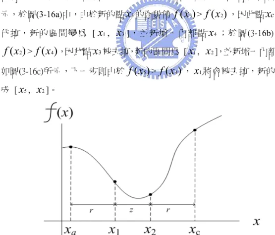
c的距離； 第二步則是重複縮小區間的過程，也就是在每一次iteration 中，藉由移除一個 邊界點與決定一個新的內部點的擺放位置，不斷地縮小區間直到達到預期的精 確度為止，另外，在每一次iteration 中，黃金分割法只需計算一次函數值，即 可將區間大小減小為原本的1-0.382 = 0.618 倍。縮小區間的過程如圖(3-16)所 示，於圖(3-16a)中，由於新的點

x

3的函數值

f x

( )

3 >

f x

( )

2 ，因此點

x

c會被取 代掉，新的區間變為 [

x

1,

x

3]，並新增一內部點

x

4；於圖(3-16b)，由於 2

( )

f x

>

f x

( )

4 ，因此點

x

3被去掉，新的區間為 [

x

1,

x

2]，並新增一內部點

x

5， 如圖(3-16c)所示，下一步則由於

f x

( )

5 >

f x

( )

4 ，

x

1將會被去掉，新的區間變 成 [

x

5,

x

2]。

Fig. 3-16. Interval reduction. 以下為黃金分割法的演算法形式，其中區間 [

x

a,

x

c] 為經由區間定位步 驟所得到的起始區間，tol 表示包含極小值的區間精確度，最後輸出的極小點位 置以滿足此精確度的最小區間的中點表示 [14]，圖(3-17)為流程圖： Algorithm 3-3: 以黃金分割法尋找函數 f 的極小值位置 Input: 起始區間 [

x

a,

x

c] 函數 f Output: 函數 f 的極小值位置

x

m

Step 1: 設區間精確度 tol. 設r = 0.382 設

x

1

= +

x

a

r x

(

c

−

x

a

)

2 c

(

c a

)

x

=

x r x

−

−

x

計算函數值

f x

( )

1 與

f x

( )

2

Step 2: WHILE (

x

c－

x

a ) > tol

IF

f x

( )

1 <

f x

( )

2 ( ) ( ) f x2 = f x1 c

x

=

x

2 2

x

=

x

1 1 a

(

c a

)

x

= +

x

r x

−

x

1 Compute

f x

( )

ELSE ( ) ( ) f x1 = f x2 a

x

=

x

1 1

x

=

x

2 2 c

(

c a

)

x

=

x r x

−

−

x

2 Compute

f x

( )

END END Step 3:輸出

x

m = 2 a c

x

+

x

，演算法停止

Fig. 3-17. Flowchart of Golden Section Search.

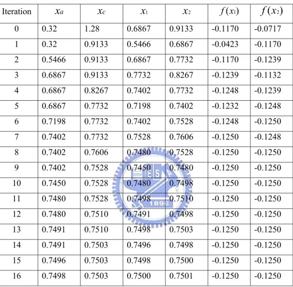
Example

以下延續上一小節區間定位步驟的範例，繼續以黃金分割法來找出函數極 小值的位置，輸入為

f x

( ) 2

=

x

2

− +

3

x

1

_{，起始區間為 [0.32, 1.28]，並依Matlab} Toolbox的初始預設值將區間精確度tol設為 0.0005，整個疊代運算的過程如表 (3-4)所示，可以發現在iteration 16 的時候，區間 [

x

a,

x

c] = [0.7498, 0.7503]，已

經 到 達 精 確 度 要 求 ， 因 此 演 算 法 結 束 ， 並 輸 出 函 數 最 小 值 的 位 置

x

m = 0.7498 0.7503 0.75 2 + ≈ 。

Table 3-4. Computation process of Golden Section Search.

Iteration

x

a

x

c

x

1

x

2 f x( )1

f x

( )

2 0 0.32 1.28 0.6867 0.9133 -0.1170 -0.0717 1 0.32 0.9133 0.5466 0.6867 -0.0423 -0.1170 2 0.5466 0.9133 0.6867 0.7732 -0.1170 -0.1239 3 0.6867 0.9133 0.7732 0.8267 -0.1239 -0.1132 4 0.6867 0.8267 0.7402 0.7732 -0.1248 -0.1239 5 0.6867 0.7732 0.7198 0.7402 -0.1232 -0.1248 6 0.7198 0.7732 0.7402 0.7528 -0.1248 -0.1250 7 0.7402 0.7732 0.7528 0.7606 -0.1250 -0.1248 8 0.7402 0.7606 0.7480 0.7528 -0.1250 -0.1250 9 0.7402 0.7528 0.7450 0.7480 -0.1250 -0.1250 10 0.7450 0.7528 0.7480 0.7498 -0.1250 -0.1250 11 0.7480 0.7528 0.7498 0.7510 -0.1250 -0.1250 12 0.7480 0.7510 0.7491 0.7498 -0.1250 -0.1250 13 0.7491 0.7510 0.7498 0.7503 -0.1250 -0.1250 14 0.7491 0.7503 0.7496 0.7498 -0.1250 -0.1250 15 0.7496 0.7503 0.7498 0.7500 -0.1250 -0.1250 16 0.7498 0.7503 0.7500 0.7501 -0.1250 -0.1250

3.2.2 Training Process Using Conjugate Gradient Method

由以上的討論可以整理出，以共軛梯度倒傳遞演算法，應用於訓練類神經 網路的過程，就是在每一次iteration 中，首先要計算搜尋的方向，然後再沿著 此搜尋方向，尋找要更新的權重值向量，其中，搜尋的方向是經由公式(3-29) 或(3-31)計算得來，而更新的權重值向量則可由黃金分割法計算而來。 當應用黃金分割法於類神經網路時，同樣依照區間定位與區間縮小兩步 驟，來尋找更新的權重值向量。區間定位步驟是從目前的權重值向量 w 開始， 計算該點的網路誤差函數值E(w)，接著是計算第二點的網路誤差函數值，它與