利用外來資訊轉換圖設計第一類混合自動重傳之位元對應在位元交錯調變碼之迭代解碼系統

國

立

交

通

大

學

電信工程學系

碩

碩

碩

碩

士

士

士

士

論

論

論

論

文

文

文

文

利用外來資訊轉換圖設計第一類混合自動重傳之

位元對應在位元交錯調變碼之迭代解碼系統

EXIT-Chart Based Labeling Design for Type-I

HARQ in BICM-ID Systems

研 究 生：蔡文傑

指導教授：沈文和 教授

中

中

中

中

華

華

華

華

民

民

民

民

國

國

國

國

九

九

九

九

十

十

十

十

六

六

六

六

年

年

年

年

九

九

九

九

月

月

月

月

利用外來資訊轉換圖設計第一類混合自動重傳之位元對應在

位元交錯調變碼之迭代解碼系統

EXIT-Chart Based Labeling Design for Type-I

HARQ in BICM-ID Systems

研 究 生：蔡文傑 Student：Wen-Chieh Tsai

指導教授：沈文和 Advisor：Dr. Wern-Ho Sheen

國 立 交 通 大 學

電 信 工 程 學 系

碩 士 論 文

A Thesis

Submitted to Institute of Communication Engineering College of Electrical Engineering and Computer Science

National Chiao Tung University in partial Fulfillment of the Requirements

for the Degree of Master of Science

in

Communication Engineering September 2007

Hsinchu, Taiwan, Republic of China

利用外來資訊轉換圖設計第一類混合自動重傳之位元對應在

位元交錯調變碼之迭代解碼系統

學生：蔡 文 傑 指導教授：沈文和 博士

國立交通大學電信工程學系﹙研究所﹚碩士班

摘

要

在現代的無線通訊系統中，位元交錯調變碼被利用來克服瑞雷（Rayleigh）衰減通 道，而混和自動重傳機制則可用來提升系統的吞吐量，兩者均是下一世代通訊系 統所採用的重要技術。在本論文中，我們針對第一類混和自動重傳機制（Type-I Hybrid Auto-retransmission Request）在位元交錯調變碼之迭代解碼（BICM-ID） 系統架構下提出一個位元對應（Labeling）及解碼器（Decoder）設計的方法。利 用外來資訊轉換圖（EXIT Chart）這個強大的工具，我們提出一個可根據外部錯 誤更正碼來設計重傳時所用位元對應的演算法。根據所找出的位元對應，我們利 用鏈路調節（Link adaptation）的概念在不同的通道訊雜比（SNR）下使用不同的 位元對應來的到較佳的品質。最後，我們根據3GPP的渦輪碼（Turbo Code）提 出一個新穎的解碼器設計，結合適當的位元對應具有優於現今3GPP規範裡設計 的品質

EXIT-Chart Based Labeling Design for Type-I

HARQ in BICM-ID Systems

Student

：

Wen-Chieh Tsai Advisors

：

Dr. Wern-Ho

Sheen

Department of Communication Engineering

National Chiao Tung University

ABSTRACT

In modern wireless communication systems, bit-interleaved coded modulation （BICM）is used to overcome the Rayleigh fading channel, and the HARQ (Hybrid Auto-retransmission Request) technique is used to improve the system throughput. In this thesis, we propose new labeling and decoder designs for Type-I HARQ for BICM-ID systems. Based on the EXIT (Extrinsic Information Transfer) chart, we develop as algorithm to search for good labeling for retransmission that well matches with the outer cod. The concept of link adaptation is realized by using different labeling at different SNR (signal to noise ratio) to achieve a better performance. Finally, a novel decoding strategy is proposed along with the proposed labeling design for turbo code in 3GPP specification. It is shown that the new design outperforms the existing one.

致謝

本篇論文得以完成首先要感謝我的指導教授

沈文和博士，在兩年

做研究過程中，給予我非常多而且重要的指導，得以研究解決有意義

的問題，並使我了解研究做學問所該具有的謹慎態度；另外，要感謝

王忠炫教授，在每星期的集會中給予我許多受用的建議及做研究的方

向；也要感謝口試委員陳仁智博士的指正與建議，讓本論文更加完善。

在此也要感謝實驗室的同學學長們，時常與我共同討論論文上遇到

的問題，在許多次反覆的討論下，得以找出解決問題的最好方法，讓

論文得以順利完成。

最後要感謝我的家人，在這兩年的過程中不斷的鼓勵我支持我，讓

我生活無憂無慮得以專心做研究，遇到問題也可以讓我有休息的機

會，好好整理心情再出發，無論遇到如何的挫折都會陪我一起度過難

關，謝謝你們。

民國九十六年九月 研究生蔡文傑謹致於交通大學

Contents

摘要

Abstract

致謝

Lists of Tables

Lists of Figures

Chapter 1

：

：

：

：

Introduction ... 1

Chapter 2

：

：

：

：

Basic Concep... 4

2.1 Hybrid ARQ（HARQ）[12] ... 4

2.1.1 Type-I HARQ... 5

2.1.2 Type-II HARQ ... 6

2.1.3 Type-III HARQ ... 6

2.2 Throughput in HARQ system ... 7

Chapter 3

：

：

：

：

System Model ... 9

3.1 System Model of HARQ in BICM-ID ... 9

3.1.1 Bit Level Inter-leaver ... 9

3.1.2 Modulator... 10

3.2 Iterative Decoding... 11

3.2.1 Detector ... 11

3.2.2 Decoder ... 13

Chapter 4

：

：

：

：

Extrinsic Information Transfer Curve

（

（

（

（

EXIT

）

）

）

）

Chart

...18

4.1.1：Transfer Characteristic ... 18

4.1.2：Transfer Curve of Decoder... 21

4.1.3：Transfer Curve of Detector ... 22

4.1.4：EXIT Chart... 26

Chapter 5

：

：

：

：

The Proposed Searching Algorithm...29

5.1.2 Binary Symmetric Extrinsic Channel... 32

5.1.3 Closed-form EXIT function ... 33

5.2 Searching Algorithm ... 36

5.3 Simulation Results ... 40

5.3.1 CC（1338,1718）, 16QAM, Rayleigh channel...40

5.3.2 CC（1338,1718）, 8PSK, Rayleigh channel...45

Chapter 6

：

：

：

：

Design for 3GPP Turbo Code...48

6.1 HARQ in 3GPP for Turbo Code ... 48

6.2 Labeling Design for Turbo Code ... 50

6.3 Novel Decoder Design for Turbo Code ... 53

6.4 Analysis of Conventional and Modified Decoder... 54

6.4.1 Information theoretical point of view ... 54

6.4.2 Numeric Values ... 56

6.5 Simulation Results ... 58

Chapter 7

：

：

：

：

Conclusions...61

List of Tables

Table 5.1 Table used for searching algorithm... 38

Table 5.2. Simulation parameter of CC（1338 , 1718） ...40

Table 5.3 Strategy of link adaptation for CC（1338 , 1718）with 16-QAM ...41

Table 5.4 Strategy of link adaptation for CC（1338 , 1718）with 8-PSK ...45

Table 6.1 Mapping functions for constellation rearrangement ... 50

Table 6.2 Mapping functions for our design, (a) candidates for second transmission and the optimal one, (b) candidate for third transmission and the optimal one ... 51

Table 6.3 Analysis in information theoretically point of view for conventional scheme and modified scheme ... 55

List of Figures

Fig. 2.1 Block diagram of Type-I HARQ ... 5

Fig. 2.2 Block diagram of Type-II HARQ... 6

Fig. 2.3 Block diagram of Type-III HARQ ... 7

Fig. 3.1 BICM with Type-I HARQ System Model... 9

Fig. 3.2 16QAM and 8-PSK constellations and the corresponding Gray labeling... 10

Fig. 3.3 BICM-ID System Model ... 11

Fig. 4.1 Soft-input-soft-output（SISO）decoder（a）and detector（b） ... 19

Fig. 4.2 the relation between IA and

σ

A ... 20

Fig. 4.3 Transfer curves of several convolutional code with distinct constrain length and of 3GPP turbo code... 22

Fig. 4.4 Block diagram of detector（demapper） ... 22

Fig. 4.5 Transfer curves of several labeling in AWGN and Rayleigh fading channel... 25

Fig. 4.6 Transfer curves of Gray labeling under distinct channel condition（SNR）... 26

Fig. 4.7 Example of trajectory under iterative decoding ... 28

Fig. 4.8 Transfer curves of distinct labeling under identical channel condition（SNR）28 Fig. 5.1 Capacity for real communication channel and virtual channel （AWGN） ... 32

Fig. 5.2 Capacity for real communication channel and virtual channel （Rayleigh）... 32

Fig. 5.3 Binary Symmetric Extrinsic Model... 33

Fig. 5.4 Two transmissions for 16QAM under Rayleigh fading channel ... 35

Fig. 5.5 Three transmissions for 16QAM under Rayleigh fading channel... 35

Fig. 5.6 Transfer curves of several labeling pair with fixed 1st mapping function ... 37

Fig. 5.7 Transfer curves of the suitable labeling in our design for CC（1338 , 1718）with 16-QAM... 42

Fig. 5.8 Throughput and PER of the suitable labeling for CC（1338 , 1718）with 16-QAM under T = 2... 43

Fig. 5.9 Throughput of the suitable labeling for CC（1338 , 1718）with 16-QAM under T = 3 ... 44

Fig. 5.10 Throughput and PER of the suitable labeling for CC（1338 , 1718）with 8-PSK under T = 2... 46

Fig. 5.11 Throughput and PER of the suitable labeling for CC（1338 , 1718）with 8-PSK with 8-PSK under T = 3 ... 47

Fig. 6.1 Transfer curves of labeling of chase combining and constellation rearrangement. ... 49

Fig. 6.2 Transfer curves of labeling of chase combining and our design. ... 52

Fig. 6.3 System model of BICM-ID with turbo code ... 53

Fig. 6.4 System model of BICM-ID with turbo code ... 55

Fig. 6.5 Mutual information between information bit and 1st decoder extrinsic ... 57

Fig. 6.7 Trajectory of iterative decoding in our design... 58

Fig. 6.8 BER of constellation rearrangement（□）and our design（○）... 59

Fig. 6.9 PER of constellation rearrangement（□）and our design（○） ... 60

Chapter 1：

：

：

：Introduction

Since 1982, when Ungerboeck proposed trellis-coded modulation（TCM）mainly for AWGN channels [1], it has been generally accepted that coding and modulation should be jointly designed for a better system performance. A symbol inter-leaver is applied to increase diversity order to the minimum number of distinct symbols between two code-words. However, when the channel is Rayleigh faded, the code performance depends strongly on its minimum Hamming distance（code diversity）rather than the minimum Euclidean distance of the code [2]. Zehavi proposed a coding modulation scheme, called BICM （Bit-Interleaved Coded Modulation）, to increase the code diversity by introducing a bit inter-leaver between encoder and modulator [3]. In [4], the author discovered that using iterative decoding with well-designed labeling the performance of BICM can be improved dramatically. Up to now, BICM has been extensively employed in practical wireless communication systems, such as HSDPA [5] and WiMAX [6].

Hybrid ARQ（Auto-retransmission Request）[4] is an another important technique in modern wireless communication systems. It combines the property of forward error control coding （FEC） and ARQ. Roughly speaking, there are three types of HARQ schemes, including chase combining（Type-I）[7], full incremental redundancy （Type-II） [8] and partial incremental redundancy（Type-III）. HARQ provides high system reliability, and thus system throughput can be enhanced substantially. HSDPA and WiMAX both employ this technique to attain good performance. Furthermore, HSDPA also utilizes different labeling in HARQ for

retransmissions to gain additional performance enhancement.

EXIT chart proposed by Brink [9] is a powerful tool to analyze convergence behavior of iterative decoding. It uses mutual information between extrinsic output and the corresponding bits to predict the performance of iterative decoding system precisely. Frequently, EXIT chart is used to design turbo code, LDPC code and BICM-ID systems.

In this thesis, EXIT chart is employed to design HARQ for BICM-ID systems. In particular, new labeling that well matches the outer code is design to improve performance. Using labeling obtained in [10] for the first transmission, an algorithm is proposed to search for good labeling for the subsequent transmissions. Link adaptation is realized by using different labeling at different SNR to further improve the performance. In addition, a new decoding method along with new labeling is proposed for the Type-I ARQ with the 3GPP turbo codes. Numerical results shoe that 0.3-0.4 dB improvement is achieved at a sight expense of decoding complexity.

The rests of the thesis is organized as follow. In Chapter 2, we introduce the concept of HARQ and discuss the important parameters to evaluate its performance, In Chapter 3, a system model for HARQ with different labeling for retransmission in BICM-ID system is introduced. In Chapter 4, we explain the EXIT chart of detector and decoder in detail. In Chapter 5, a simplified model for EXIT chart and a searching algorithm are proposed, and a number of simulation results are given for various coding and modulation schemes. In chapter 6, we

Chapter 2：

：

：

：Basic Concep

2.1 Hybrid ARQ（

（

（HARQ）

（

）

）

）[12]

Forward Error Control（FEC）and Auto-retransmission Request（ARQ）schemes are two techniques for controlling transmission error in data transmission systems. In a FEC system, a good error-correcting code is used. While the receiver detects the presence of errors in a received packet, it attempts to determine the error locations and then corrects those errors. After decoding, the receiver accepts the packet no matter it is error-free or erroneous. In an ARQ system, a code with good error-detecting capability is used. If the received packet is detected as error-free, it will be accepted by the receiver. At the same time, the receiver sends a positive acknowledgment（ACK）to transmitter via a return channel to notify that the packet has been successfully received. If the received packet is detected as erroneous, the receiver send a negative acknowledgment（NACK）to transmitter and request transmitter to retransmit the same packet. Retransmission continues until either that the packet is successfully received or that errors repeatedly occur to the maximum retransmission number for that packet.

Comparing FEC with ARQ, we see that ARQ is simple and provides high system reliability, however, throughput of ARQ falls rapidly with increasing channel error rate. FEC keeps higher throughput than ARQ, but it is hard to achieve high system reliability because the probability of decoding error is much greater than probability of an undetected error.

FEC and ARQ can combined properly to exploit respective advantages and overcome drawbacks. Such a combination of the two schemes is referred as a hybrid ARQ.

2.1.1 Type-I HARQ

As shown in Fig.2.1, In the Type-I HARQ scheme if the receiver fails to decode the transmit coded packet, a retransmission request, NACK, is fed back from receiver to transmitter. Upon reception of this NACK, the transmitter sends the same coded packet again. The receiver needs to buffer all previously received packets and combine those with recently received packet according to maximal ratio combining（MRC）, which was first discussed by Chase [7]. Hence, the Type-I HARQ is also referred to “Chase combining”（CC）.

Type-I HARQ provides diversity gain by decoding a packet because of combining multiple received signals. To perform Type-I HARQ, it needs only additional buffer to save received packets compared with the conventional ARQ, but the feedback and decoding schemes are the same as those in the conventional ARQ.

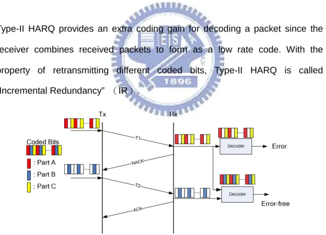
2.1.2 Type-II HARQ

In real communication systems, coded bits coming out from encoder need to be punctured before transmission in order to improve the bandwidth efficiency. Type-II HARQ utilizes the property of punctured code. As in Fig. 2.2, the coded bits are punctured to three parts A, B and C. At the first transmission, transmitter sends punctured coded bits A and B to receiver for example. If the receiver fails to decode the packet, the transmitter sends additional coded bits, that is, the redundant bits C Instead of sending the same coded packet, the transmitter sends additional coded parts, when a NACK is received.

Type-II HARQ provides an extra coding gain for decoding a packet since the receiver combines received packets to form as a low rate code. With the property of retransmitting different coded bits, Type-II HARQ is called “Incremental Redundancy” （IR）.

Fig 2Fig. 2.2 Block diagram of Type-II HARQ

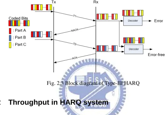
only redundant bits but identical bits. The identical bits are combined using MRC, and the redundant bits are exploited to form a lower rate code with stronger error correction capability. Type-III HARQ inherits the advantages of Type-I and Type-II HARQ and is called “Partial Incremental Redundancy”. Fig. 2.3 shows theblock diagram of Type-III HARQ.

Fig 3Fig. 2.3 Block diagram of Type-III HARQ

2.2 Throughput in HARQ system

A key performance metric for HARQ is its throughput, which is the number of bits conveyed per unit time. In a type-I HARQ system, the information we want to deliver are encoded as binary coded bits sequence, namely, data packet. During the HARQ process, a data packet can be sent to the receiver using M transmission packets at most, that is M is the maximum transmission number for a data packet. Suppose modulation scheme is identical during retransmission, the throughput of type-I HARQ can be calculated as follow. Assume N is the number of data packets sent to the receiver. The throughput is given by

(

)

= ∗ = # inf / sec # #

of successfully received ormation bits Throughput bits

Time to deliver N data packets

of successfully received data packet r of transmitted transmission packet ∗ R ,

where r is the code rate, and R is the packet transmission rate. Since r and R are fixed, we define another metric Ψ in place of throughput for convenience.

Ψ = # , 0≤ Ψ ≤1

#

of successfully received data packet of transmitted transmission packet

Chapter 3：

：

：

：System Model

3.1 System Model of HARQ in BICM-ID

Fig.3-1 shows the system model of BICM with Type-I HARQ. A binary information data

b

is encoded as codeword

c

, and a bit level inter-leaver

Π

located between encoder and modulator converts

c

to a bit sequence

c

'

. The

modulation scheme has an M-ary constellation signal set

χ

=

{

x

₁

,

…

,

x

_M

}

with

2

m

M

=

.

c

'

is put into modulator sequentially and every m bits are grouped to form a label

s

=

[

c

₀

,

…

,

c

_m-1

]

. Let

Λ

be the set of all possible labels,

2

m

=

Λ

.Through the modulator, a constellation point

x

=

µ

( )

s

is selected according to a labeling mapping function

µ

.

µ

_i represents the mapping function used in i-th transmission.

b

c

c

'

'

c

1

x

M

x

1

y

T

y

Fig 4Fig. 3.1 BICM with Type-I HARQ System Model

3.1.1 Bit Level Inter-leaver

The inter-leaver used in the system is S-random inter-leaver [13]. An S-random interleaver guarantees that the two bits within a distance S1 at the interleaver

input can not be mapped to a distance less than S2 apart at the interleaver

Define an interleaving function

π

: c_j =c'_{π( )j} . If

i − <j S （3-1） Then the design guarantees that

π

( ) ( )

i −π j >S （3-2）

3.1.2 Modulator

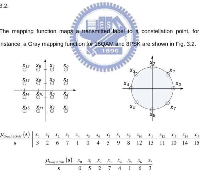
The coded bits coming out from encoder followed by bit inter-leaver are grouped every m bits and mapped to constellation point by specific mapping function. In the thesis, we consider only 16-QAM and 8PSK constellations as shown Fig. 3.2.

The mapping function maps a transmitted label to a constellation point, for instance, a Gray mapping function for 16QAM and 8PSK are shown in Fig. 3.2.

x0 x1 x2 x3 x4 x5 x6 x7 x8 x9 x10 x11 x12 x13 x14 x15

( )

,16 0 1 2 3 4 5 6 7 8 9 10 11 12 13 14 15 3 2 6 7 1 0 4 5 9 8 12 13 11 10 14 15 Gray QAM x x x x x x x x x x x x x x x x

µ

s s

( )

,8 0 1 2 3 4 5 6 7 0 5 2 7 4 1 6 3 Gray PSK x x x x x x x x µ s s

3.2 Iterative Decoding

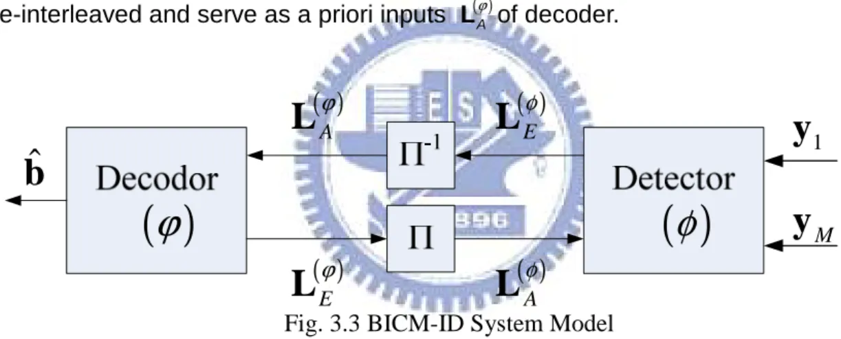
Since the optimal decoding strategy for BICM system, that is, MAP, is too complex to implement, we separate the receiver into two parts：detector and decoder. And the detector and the decoder exchange soft information iteratively.

Fig. 3.3 shows a diagram of iterative decoding for BICM HARQ. The detector φ takes channel outputs y₁,…,y , and intrinsic LLRs from decoder , _M L , to ( )_Aφ

compute extrinsic LLRs, L( )_Eφ . Then, the extrinsic LLRs of detector are de-interleaved and serve as a priori inputs L of decoder. ( )_Aϕ

Fig 6Fig. 3.3 BICM-ID System Model

3.2.1 Detector

The APP detector is used to compute the a posteriori probability for coded bits. Since memory-less modulation scheme is used, we demodulate received signal symbol by symbol. The APP for bit c_i in a symbol, L( )_Dφ

( )

i is

( )

φ

( )

ϕ

( )

E φ

L

( )

E ϕ

L

( )

A ϕ

L

( )

A φ

L

1

y

M

y

ˆ

b

( )

_{( )}

(

)

(

)

(

)

(

)

₍

(

)

₎

( )

_{( )}

(

) (

)

(

) (

)

( )

_{( )}

(

)

1 0 1 1 1 1 1 1 1 Pr 1 , , log Pr 0 , , Pr , , 1 Pr 1 log log Pr 0 Pr , , 0 Pr , , 1, Pr 1 log Pr , , 1, Pr 0 Pr 1 Pr , , log φ φ φ ∈ ∈ = … = = … … = = = + = … = … = = = + … = = = … = +

∑

∑

i i i T D i T T i i i T i T i i s A T i i s i T A c y y L i c y y y y c c c y y c y y c s s c L i y y c s s c s c y y L i Λ Λ

(

)

(

) (

)

1 0 1 1 1 ( ), , ( ) Pr 0 Pr , , ( ), , ( ) µ µ µ µ ∈ ∈ = …

∑

∑

… … i i T s i T T s s s s c y y s s Λ Λ ( )

_{( )}

( )

_{( )}

( )

_{( )}

( )

_{( )}

( )

_{( )}

1 0 1 1 2 0 1 1 2 0 ˆ _{( )} exp exp log ˆ _{( )} exp exp φ φ φ φ φ µ σ µ σ − = = ∈ ≠ − = = ∈ ≠     _{ − }   _{ }   _{ }         = +     _ − _   _{ }   _{ }         = +

∑

∑

∑

∑

∑

∑

i i T k k k m s k j A j s j i A T k k k m s k j A j s j i A E y h s c L j L i y h s c L j L i L i Λ Λ

( )

3-3 where b i

Λ is the set of labels whith i-th bit equal to b, and cs_j is j -th bit of label s.

The APP detector can be approximated by the max-log detector in order to reduce decoding complexity. From e.q.（3-3）, the max-log detector can be written as

( )

_{( )}

( )

_{( )}

( )

_{( )}

( )

_{( )}

( )

_{( )}

( )

_{( )}

1 0 1 1 1 2 0 1 1 2 0 1 0 ˆ _{( )} exp exp log ˆ _{( )} exp exp max exp log φ φ φ φ φ φ µ σ µ σ − = = ∈ ≠ − = = ∈ ≠ − ∈ ₌ ≠     _{ − }   _{ }   _{ }         = +     _{ − }   _{ }   _{ }             ≈ +

∑

∑

∑

∑

∑

∑

∑

i i i T k k k m s k j A j s j i D A T k k k m s k j A j s j i m s j A s _j j i A y h s c L j L i L i y h s c L j c L j L i Λ Λ Λ ( )

_{( )}

( )

_{( )}

( )

_{( )}

0 1 1 2 1 1 2 0 1 1 2 0 ˆ _{( )} exp ˆ _{( )}

max exp exp

ˆ _{( )} max φ φ φ µ σ µ σ µ σ = − = ∈ ₌ ≠ − = ∈ ₌ ≠     −     _{  }  _       _{  }  _{ }        −     _{   }  _{ }       _{   }  _{ }    −  = +  +

∑

∑

∑

∑

∑

i i T k k k k T k k k m s k j A s _j j i T k k k m s k A j A s j j i y h s y h s c L j y h s L i c L j Λ Λ ( )

_{( )}

(

)

0 1 1 2 0 ˆ _{( )} - max 3 4 φ µ σ − = ∈ ₌ ≠    −       +                −

∑

∑

i T k k k m s k j A s j j i y h s c L j Λ

3.2.2 Decoder

In the BICM-ID system, a SISO decoder is needed to compute soft information passed to detector. In the thesis, BCJR algorithm [14] is utilized.

The log-APP of coded bit c_j, L( )_Dϕ

( )

c_j is written as ( )

( )

( )

(

)

( )

(

)

Pr 1 log Pr 0 j A D j j A c L c c ϕ ϕ ϕ = = L L ≜ _（3-5）

Then, making use of the trellis structure of convolutional code, equation (3-5) can be reformulated as

( )

( )

( )

(

)

( ) ( )

(

)

( ) 1 0 1 ', 1 ', Pr ', , log Pr ', , l l l l A s s D j l l A s s s s s s L c s s s s ϕ ϕ ϕ + ∈Σ + ∈Σ = = = = =

∑

∑

L L （3-6） b l

Σ is the set of state pairs that correspond to the coded bit c_j =b at time l .

Next we show how the joint probability in (3-6) can be evaluated recursively.

( )

(

)

( )

₍

₎

( )

_{( )}

( )

₍

₎

(

)

( )

₍

₎

( )

₍

₎

( )

_{( )}

(

)

(

( )

_{( )}

( )

₍

₎

)

(

( )

₍

₎

)

( )

₍

₎

(

)

(

( )

_{( )}

)

(

( )

₍

₎

)

_{( )}

1 Pr ', , Pr ', , , = , Pr ', , , = Pr , = ', Pr ', Pr Pr , = ' Pr ', 3-7 ϕ ϕ ϕ ϕ ϕ ϕ ϕ ϕ ϕ ϕ ϕ ϕ ϕ + = = = < > = > < < < = > < l l A A A A A A A A A A A A A s s s s s s t l t l t l t l s s t l t l s t l s t l s t l t l s s t l s s t l L L L L L L L L L L L L L

where L( )_Aϕ

(

t >l

)

represents the portion of a prior LLRs after time l, and

( )

₍

₎

A t l

ϕ _<

L the portion of a prior LLRs before after time l. The last equality follows from the fact that the probability of the state at time l depends only on the previous states before time l.

Defining

( )

(

( )

₍

₎

)

(

)

(

( )

_{( )}

)

( )

(

( )

₍

₎

)

1 ' Pr ', ', Pr , = ' Pr ϕ ϕ ϕ α γ β+ < > l A l A l A s s t l s s s t l s s t l s L L L ≜ ≜ ≜ We can write (3-7) as Pr

(

s_l =s s', _l+1=s,L( )ϕ_A

)

=

β

_l+1

( ) (

s ⋅

γ

_l s s',

) ( )

⋅

α

_l s' （3-8） , and we can write the branch metric

γ

_l

(

s s',

)

as

(

)

(

( )

_{( )}

)

(

)

( )

( )

₍

₎

(

)

(

)

( )

(

( )

₍

₎

)

( )

-1

(

( )

( )

)

0 ', Pr , = ' Pr ', , Pr ', Pr ' Pr ', Pr ' Pr ', Pr ' Pr l A A A k A j j j s s s t l s s s t l s s s s s s s t l s s s s L c c ϕ ϕ ϕ ϕ γ =  ₌   _{ } = _{ }    _{  } = = =

∏

L L L ≜ （3-9） Where ( )

( )

(

)

(

(

( )( )

( )

( )

)

)

( )

( )

(

)

(

( )

( )

)

exp Pr 1 1 exp 1 Pr 0 1 exp A j A j j A j A j j A j L c L c c L c L c c L c ϕ ϕ ϕ ϕ ϕ = = + = = +

Thus, we can compute a forward metric

α

_l+1

( )

s' for each state s' at time l+1 using the forward recursion method as

( )

(

( )

₍

₎

)

(

( )

₍

₎

)

( )

₍

₎

( )

₍

₎

(

)

(

( )

₍

₎

)

( )

₍

₎

(

)

(

( )

₍

₎

)

(

) ( )

1 ' Pr ', 1 = Pr , ', 1 Pr ', , Pr , Pr ', Pr , ', ' l l l l l A A s A A A s A A s l l s s s t l s s t l s t l s t l s t l s t l s s t l s s s ϕ ϕ σ ϕ ϕ ϕ σ ϕ ϕ σ σ α γ α + ∈ ∈ ∈ ∈ = < + < + = = < < = = < =

∑

∑

∑

∑

L L L L L L L （3-10）

Where σ_l is the set of all states at time t. A backward metric

β

_l

( )

s for each state s at time l using the backward recursion method as

( )

(

( )

₍

₎

)

(

( )

₍

₎

)

( )

₍

₎

(

)

(

( )

₍

₎

)

(

)

( )

(

)

2 1 1 1 2 1 ' 2 1 1 ' 1 +2 ' Pr Pr , ' Pr 1 , ' Pr 1 ', ' 3 - 11 ϕ ϕ σ ϕ ϕ σ σ β γ β + + + + + + ∈ + + + ∈ + ∈ > = > = = = = + = = > + = =

∑

∑

∑

l l l l A A l l s A l l A l s l l s s t l s t l s s s s t l s s s s t l s s s s s L L L L ≜

Therefore, according to equation (3-9), (3-10), and(3-11),the log-APP of coded bit c can be written as _j

( )

( )

( )

( ) (

) ( )

( ) (

) ( )

( )

( ) ( )

( )

(

( )

_{( )}

)

( )

( ) ( )

( )

(

( )

_{( )}

)

( ) ( )

( )

(

)

( )

( )

(

)

1 0 1 0 1 ', 1 ', -1 1 0 ', -1 1 0 ', ', ' log ', ' ' Pr ' Pr log ' Pr ' Pr Pr =1 log +log Pr =0 ϕ ϕ ϕ ϕ ϕ β γ α β γ α β α β α β + ∈Σ + ∈Σ + = ∈Σ + = ∈Σ + ⋅ ⋅ = ⋅ ⋅ ⋅ ⋅ = ⋅ ⋅ =

∑

∑

∑

_∏

∑

_∏

l l l l l l l s s D j l l l s s k l l A i i i s s k l l A i i i s s l A j j A j j s s s s L c s s s s s s s s L c c s s s s L c c L c c L c c

( ) ( )

( )

(

( )

_{( )}

)

( )

( ) ( )

( )

(

( )

_{( )}

)

( ) ( )

( )

( )

( )

₍

₎

1 0 -1 1 0 ', -1 1 0 ', ' Pr ' Pr ' Pr ' Pr 3 12 ϕ ϕ ϕ ϕ α β α = ∈Σ ≠ + = ∈Σ ≠ ⋅ ⋅ ⋅ ⋅ = + −

∑

_∏

∑

_∏

l l k l A i i i s s i j k l l A i i i s s i j A j E j s s s s L c c s s s s L c c L c L c

The extrinsic LLRs are then passed to detector for next iteration of processing.

After iteratively processing is terminated, we decode information bits by using a posteriori LLRs with hard decision. The a posteriori LLRs of information bit b is _n

( )

( ) (

) ( )

( )

( ) (

) ( )

( ) 1 0 1 ', 1 ', ', ' log ', ' l l l l l s s D n l l l s s s s s s L b s s s s

β

γ

α

β

γ

α

+ ∈Ω + ∈Ω ⋅ ⋅ = ⋅ ⋅

∑

∑

（3-13）

where Ωb_l is the set of state pairs that corresponds to the information bit b_n =b at time l . And we decode information bits as

( )

( )

1 , 0 ˆ 0 , 0 D n n D n L b b L b  >  = ≤  （3-14） In order to simplify the calculations, the following identity is used

( )

(

)

( )

(

)

(

)

max* , log x y max , log 1 x y 3-15

x y ≜ e +x = x y + +e− −

( )

(

( )

)

(

)

(

(

)

)

( )

(

( )

)

* * * 1 1 ' log ' ', log ', log α α γ γ β+ β+ = = = l l l l l l s s s s s s s s

Finally by using the log-domain metrics, the e.q.（3-13）can be written as

( )

( )

( ) (

) ( )

( ) (

) ( )

( ) ( )

{

( )

(

)

( )

}

( )

{

( )

(

)

( )

}

1 0 1 0 1 ', 1 ', * * * * 1 ', * * * * 1 ', ', ' log ', ' max ', ' max ', '

β

γ

α

β

γ

α

β

γ

α

β

γ

α

+ ∈Ω + ∈Ω + ∈Ω + ∈Ω ⋅ ⋅ = ⋅ ⋅ = + + − + +

∑

∑

l l l l l l l s s D n l l l s s l l l s s l l l s s s s s s L b s s s s s s s s s s s s （3.16）

The exponential terms in e.q.（3-13）have been convert to addition terms in e.q. （3-16）, and the complexity is reduced largely. To reduce computation complexity further, the “ max* “ function can be approximated as

max*

( )

x y, ≈max

( )

x y, 3-15

(

)

the decoder using the function max instead of max* is called max-log-MAP decoder. In the rests of this thesis, we consider only the max-log-MAP decoder for practical reason.

Chapter 4：

：

：

：Extrinsic Information Transfer Curve（

（

（

（EXIT）

）

）

）

Chart

In this chapter, we discuss a powerful tool, the EXIT chart, and use it to analyze the convergence behavior of iterative decoding. EXIT chart was proposed by S. ten Brink in 2001. EXIT chart depicts the relation between mutual information of intrinsic log–likelihood ratios and coded bits and that of extrinsic log–likelihood ratios and coded bits for soft input soft output（SISO）decoder（or detector）. Using mutual information transfer characteristics of SISO decoder, we can analyze the convergence behavior and design the system for better performance.

4.1.1：

：

：Transfer Characteristic

：

A SISO system is shown in Fig. 4.1. Where X is the information we transmit, that

is, coded bits sequence in BICM-ID system, LA is intrinsic soft information

and LE is extrinsic soft information about X.

First, we consider a simple case of BPSK modulation over AWGN channel. The received signal is

y = +x n （4.1） where “x” is the transmitted BPSK signal and “n” is AWGN noise with zero mean and variance σ_n2. At receiver, the log-likelihood ratio is calculated as

Fig 7Fig. 4.1 Soft-input-soft-output（SISO）decoder（a）and detector（b）

(

)

(

)

(

)

(

)

(

)

2 2 2 2 2 2 1 1 exp 2 2 Pr 1 log log Pr 1 _{1 1} exp 2 2 2 2 n n n n y y n n y y x L y x _y y x n x n

σ

πσ

σ

πσ

µ

σ

σ

 ₋  ₋    = + _{ } = =   = − ₊ ₋      = ⋅ = + = ⋅ + （4.2） where _y 2₂ n µ σ

= and n is Gaussian distribution with zero mean and variance _y

2

2

y y

σ

=

µ

.

Two observations in [9] are used：

（1） For large inter-leavers the a priori values LA remain fairly

uncorrelated form the respective channel observation over much iteration.

（2） The probability density functions of the extrinsic values LE approach

Gaussian-like distributions with increasing number of iterations.

Observations 1 and 2 suggest that the intrinsic soft information input to detector or decoder can be modeled by an independent Gaussian random variable as

(

2

)

2

, ~ 0, , 2

A A A A A A A

L =µ x+n n N σ µ =σ

(

)

2 2 2 2 1 exp 2 2 A A A A x p X x σ ξ ξ σ πσ _{ }  _{ − }     = = _{ }       （4.3）

The mutual information between transmission bit x and intrinsic LLR a is calculated as

(

)

(

)

(

)

(

)

(

)

2 -1 2 1 ; log 2 1 -1 A A A x A A P X x I I X A P X x d P X P X ξ ξ ξ ξ ξ +∞ ∞ =± ⋅ = = = = = + + =

∑ ∫

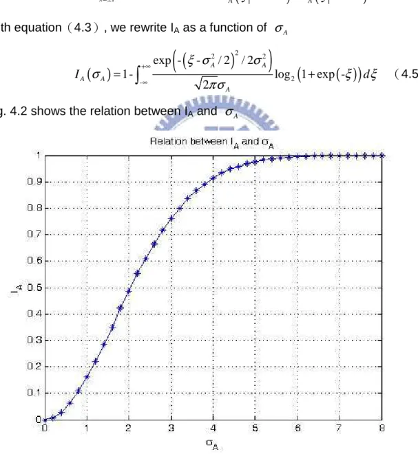
（4.4）

With equation（4.3）, we rewrite IA as a function of σA

( )

(

(

)

)

(

( )

)

2 2 2 2 -exp - - / 2 / 2 1- log 1 exp -2 A A A A A I d

ξ σ

σ

σ

ξ

ξ

πσ

+∞ ∞ =

_∫

+ （4.5）

Fig. 4.2 shows the relation between IA and σA

Fig 8Fig. 4.2 the relation between IA and σA

calculated as

(

)

(

)

2

₍

(

₎

₍

)

₎

-1 2 1 ; log 2 1 -1 A E E x E E P X x I I X E P X x d P X P X ξ ξ ξ ξ ξ +∞ ∞ =± ⋅ = = = = = + + =

∑ ∫

（4.6）

To compute IE for a desired IA, first we choose the σA according to IA and model the intrinsic input as the independent Gaussian random variable in（4.6）. Finally, we measure the mutual information between extrinsic outputs and transmission bits.

4.1.2：

：

：Transfer Curve of Decoder

：

In BICM-ID system, the outer decoder receives the log-likelihood ratios form the detector. Hence, the transfer curve of decoder only influenced by the error correction code we use.

Fig. 4.3 shows several transfer curves of max-log decoders. In EXIT Chart, the mutual information between intrinsic input and coded bits is plot on “X” axis and the mutual information between extrinsic input and coded bits is plot on “Y” axis.

It is obvious for all the decoders that the a more reliable intrinsic inputs to decoder the more reliable extrinsic the decoder outputs. In Fig. 4.3, we can see that the threshold of the extrinsic is more apparent if the code with more powerful error correcting capability. Take turbo code with eight inner iterations for instance, If the mutual information of coded bits and intrinsic is over than 0.5, the mutual information of coded bits and extrinsic increases dramatically.

Fig 9Fig. 4.3 Transfer curves of several convolutional code with distinct constrain length and of 3GPP turbo code

4.1.3：

：

：Transfer Curve of Detector

：

As shown in Fig. 4.4, the detector receives both the log-likelihood ratios（l ）_a from the decoder and signals（y₁,…,y_T）from communication channel. Random variables are written using upper case letters and their realizations by the corresponding lower case ones. Therefore, the mutual information can be written as

(

)

-1

(

)

1

( )

( )

_{( )}

, -0 0 1 1 ; ; log 2 m a A A k A k a a k c a p l c I I I X L p l c dl m p l +∞ ∞ = =   = = = _ _  

∑

∑∫

S L （4.7）

where X_k is k-th bit of transmission label s and L_{A , k} is the intrinsic LLR of X_k. The last step is true because that the intrinsic LLRs are assumed as i.i.d. Gaussian distribution as chapter 4.1.1. The mutual information between extrinsic LLR and transmission label is written as

(

)

(

)

(

[ ]

)

-1 -1 , 1 0 0 1 1 ; ; ; , , , m m k E E k E k k A T k k I I I X L I X Y Y m ₌ m ₌ = S L =

_∑

=

_∑

L … （4.8）

where L_{E , k} is extrinsic LLR of k-th bit and L[ ]k_A is m-1-tuple vector composed of the LLRs of a label except which of k-th bit. The last equation is due to the detector calculate LE , k based on only

[ ]k A L and Y1,…,YT. [ ]

(

)

( )

(

[ ]

)

[ ]

(

)

(

(

[ ]

)

)

[ ] [ ]

( )

( )

( )

(

(

[ ]

)

)

[ ] 1 1 1 1 1 1 1 1 ; , , , - , , , 1- , , , 0 , , , 1- 0 , , , k k A T k k k A T k k k A T k A T A T k k k A T k A T A T I X Y Y H X H X Y Y p y y h p x y y d dy dy p p y p y h p x y y d dy dy … = … = … = … = = …

∫ ∫ ∫

∫ ∫ ∫

L L l l l l l l ⋯ ⋯ ⋯ ⋯ ⋯ （4.9）

where h p

( )

=- logp 2

( ) (

p - 1-p

)

log 1-2

(

p

)

is the binary entropy function. The

last step is true because the transmission bits us symmetric, that is,p x

(

_k =0

)

= p x

(

_k = =1

)

0.5. With Bayer’s theorem,

(

0 [ ], 1, ,

)

k k A T p x = l y … y can be written as [ ]

(

)

[ ]

(

)

(

)

[ ]

(

)

(

)

[ ]

(

)

[ ]

(

)

1 1 1 1 0 1 1 1 0 0 , , , , , , 0 0 , , , , , , 0 , , , k k A T k A T k k k A T k k c k A T k k A T k c p x y y p y y x p x p y y x c p x c p y y x p y y x c = = = … … = = = … = = … = = … =

∑

∑

l l l l l （4.10） Therefore

[ ]

(

)

[ ]

(

)

(

)

[ ]

(

)

(

)

( ) ( )

( )

[ ]

( ) ( )

(

)

1 1 1 1 -1 1 , 0 , , , c , , , , c , , , 2 M 2 M c k c k k A T k k A T k k k A T k k T A m s T A i j i i k p y y x p y y x p x c p y y p x c p y p y p p y p y p l c ∈ ∈ ∈ = ≠ … = = … = = = … = = =

∑

∑

∑

∏

s Λ s Λ s Λ s l l s s l s s s s l s s s ⋯ ⋯ c k ∈

∑

Λ （4.11）

Using equations （4.7）~（4.11）, the I_A and I_E can be calculated exactly but complicated since it needs to compute large integration. Because it is almost impossible to compute the exact value, Monte Carlo simulation（histogram measurements）is utilized.

From equation（4.11）, we can observe that the channel condition and the mapping function are two key parameters that affect the EXIT chart of detector. Fig. 4.5 shows some results in [10] for AWGN and Rayleigh fading channels. With the observation that the transfer curves of chart of detector can be approximated to a straight lines, we define the “slope” of a transfer curve as the slope of the straight line form zero prior point（IA,detector = 0）to ideal prior point

（IA,detector = 1）. Mapping function set with various slope has been fund in [10] for

many regular modulation scheme.

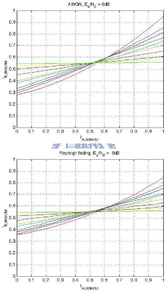
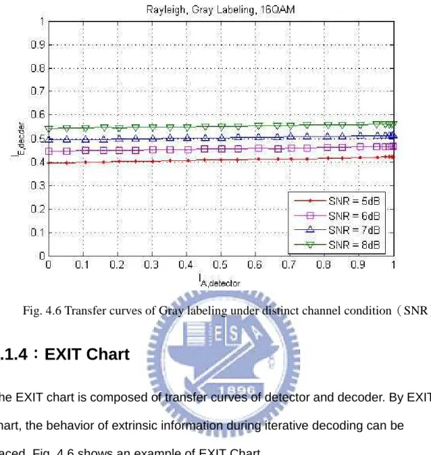
Fig. 4.6 shows the transfer curves of Gray labeling under distinct channel condition（SNR）. The transfer curves of identical labeling are approximately parallel, and the transfer curve is “higher” when SNR is larger.

Fig 11Fig. 4.5 Transfer curves of several labeling in AWGN and Rayleigh fading channel.

Fig 12Fig. 4.6 Transfer curves of Gray labeling under distinct channel condition（SNR）

4.1.4：

：

：EXIT Chart

：

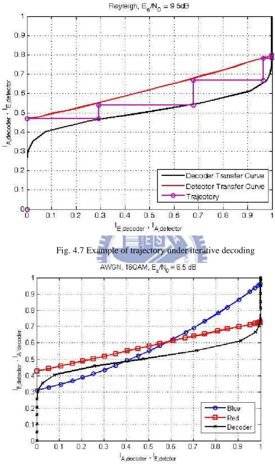
The EXIT chart is composed of transfer curves of detector and decoder. By EXIT chart, the behavior of extrinsic information during iterative decoding can be traced. Fig. 4.6 shows an example of EXIT Chart.

In Fig. 4.7, the decoder curve and the detector curve separate far enough to introduce a tunnel, the final extrinsic information of the decoder can reach the location with high reliability. In other word, the waterfall region on BER curve of iterative decoding is related to the appearance of the tunnel between detector transfer curve and decoder transfer curve. It is believed that the higher reliability of decoder output the lower bit error rate. In Fig 4.8, transfer curves of two distinct labeling under AWGN channel with identical SNR and the convolutional

point with low decoder extrinsic reliability, and the “Red” one introduce a tunnel between the detector and decoder. It is obvious that the red one has a better performance than the blue one.

Therefore, the criterion of choosing the suitable labeling is that the labeling with the tunnel appearing at as lower SNR as possible.

Fig 13Fig. 4.7 Example of trajectory under iterative decoding

Fig 14Fig. 4.8 Transfer curves of distinct labeling under identical channel condition

Chapter 5：

：

：

：The Proposed Searching Algorithm

In the chapter, we propose an algorithm to search for labeling for Type-I HARQ in order to make throughput as high as possible. First, an analytical model for EXIT Chart is introduced. With the simple model, the detector transfer curve on EXIT could be approximated accurately by a close-form function. Next, we propose a search algorithm using the concept of binary search algorithm（BSA） to establish a labeling set. Therefore, optimal labeling can be chosen according to code scheme and SNR.

5.1 Simplified Model

An analytical approximate expression for the EXIT function of a maximum a posterior probability（MAP）detector over memory-less channels under single transmission is derived in [15]. The real communication channel is replaced with a hard decision virtual channel, and the intrinsic information coming from decoder is modeled as a binary symmetric channel or a binary erasure channel. The method is modified to the case of HARQ（Multiple transmissions）.

5.1.1 Hard Decision Virtual Channel

The real communication channels considered in the thesis are AWGN and Rayleigh fading channels. Relation between transmit and receive signals can be represented as

y= ⋅h

γ

⋅ +x n （5.1） where x is the transmitted constellation point and y is the corresponding received signal. h is the fading coefficient with distribution

( )

( )

2

2 exp

-H

in Rayleigh fading channel and h=1 in AWGN channel. γ is the signal to noise ratio

0

s

E

N , and n is i.i.d. complex Gaussian noise with distribution

( )

0,1

CN .

Next, define a transmission matrix M M×

( )

γ

Q to characterize this virtual channel when SNR equal to γ . The element q_{i j,} denote transmission probability from the input signal x_i to received signal x_j if we use maximum likelihood（ML）

detection on the received signal and hard decision, ,

(

)

r t

i j j i

q = p x =x x =x

, , , 0,1, , -1

j i

x x ∈χ i j= … M . Obviously, the alphabet of output signals from real communication channel is infinite but which from virtual channel is finite. The capacity of this virtual channel is

( )

(

)

(

)

₍

(

_{) (}

)

₎

(

)

(

)

(

) (

)

-1 -1 2 0 0 -1 -1 2 -1 0 0 0 , ; , log , , log , t r M M i j t r t r hard i j _{t r} i j i j t r M M i j t r i j M r t t i j j i i k t i p X x X x C I X X p X x X x p X x p X x p X x X x p X x X x p X x X x p X x p X x

γ

= = = = =  _{= =}    = = = = _{ } = =      _{= =}    = = =  _{= = =}      = =

∑∑

∑∑

∑

(

)

(

(

)

)

(

) (

)

(

)

(

)

( )

-1 -1 2 0 0 -1 -1 2 -1 0 0 0 , 2 , 2 -1 , 0 log 1 , , log 1 log log M M r t j i i j t r M M i j t r t i j i M r t i j j i k i j i j M k j k X x p X x p X x X x p X x X x p X x p X x X x q M q M q = = = = = = = = +    _{= =}    = = =  _{= =}          = +    

∑∑

∑∑

∑

∑

( )

-1 -1 0 0 5.2 M M i= j=    

∑∑

where a constellation pointis equally likely, that is, p X

(

t xi

)

1

M

= = .

The capacity of real communication channel is

( )

(

)

(

)

₍

(

₎

_{( )}

)

(

)

_{( )}

(

_{( )}

)

( )

(

)

(

)

(

)

(

)

(

)

-1 2 0 -1 2 0 2 2 ; , , , , , log , , , 1 , , log , , , log M + , , log , t real t M i t i _t i _i M i i i i i i i i k k C I X Y H p X x y h p X x y h dydh p X x p y h p x y h p x y h dydh p x p y h p y x h p x h p y x h p x h p y x h p x γ = = =  ₌    = = _{ } =     = _ ⋅ _   =

∑∫ ∫

∑∫ ∫

(

)

( )

(

)

(

)

(

)

(

)

( )

-1 -1 0 0 -1 2 2 -1 0 0 , , log M + , , log 5.3 , M M i k M i i i M i k k dydh h p y x h p y x h p x h dydh p y x h = = = =                   =      

∑∫ ∫

∑

∑∫ ∫

∑

The last step in equation（5.3）follows that the probability of fading gain and transmitted signal are independent and transmitted signals are equally likely, that is, p x h

(

_i,

)

= p x p h

( ) ( )

_i = p x

( ) ( )

_k p h = p x h

(

_k,

)

, ∀i j, = …0, ,M −1.

A number of capacities for 16-QAM constellations over AWGN and Rayleigh fading channels are plotted in Fig. 5.1 and Fig. 5.2. It is obviously that

( )

( )

hard real

C

γ

<C

γ

. In the simplified model, a discrete channel with transmission matrix Q

( )

γ

ˆ is selected instead of real communication channel with SNR equal to γ such that C_hard

( )

γ

ˆ =C_real

( )

γ

.

Fig 15Fig. 5.1 Capacity for real communication channel and virtual channel （AWGN）

Fig 16Fig. 5.2 Capacity for real communication channel and virtual channel （Rayleigh）

corresponding extrinsic value from decoder which is served as prior in detector. The extrinsic value of any transmitted bit is either "0" or "1". The model is parameterized by the crossover probability

ε

. The transmitted bit is equally likely

(

0

)

(

1

)

1

2

p b= = p b= = , and it is obviously that

(

0

)

(

1

)

1 2

p l= = p l= = . The mutual information between b and l can be calculated as

(

)

( )

_{( ) ( )}

( )

( )

(

( )

)

( ) ( )

( )

( )

( )

( ) ( )

( )

1 1 2 0 0 1 1 2 0 0 , ; , log 1 , log 1 1- log 1- log - 1- log 1- - log b l b l p b l I B L p b l p b p l p b l p l b h h ε ε ε ε ε ε ε ε ε ε = = = =   = _ _   = + = + + = =

∑∑

∑∑

（5.4）

In the simplified model, the BSC extrinsic model is used instead of i.i.d. Gaussian model. A suitable

ε

is selected to introduce specific IA in BSC model just like that we select σ_A in i.i.d. Gaussian model.

1 -

ε

ε

ε

1 -

ε

Fig 17Fig. 5.3 Binary Symmetric Extrinsic Model

5.1.3 Closed-form EXIT function

The mutual information between coded bits and detector extrinsic has been derived in Section 4.1.3 for the communication channel with i.i.d. Gaussian prior. In the simplified model, the communication channel is replaced by a

discrete channel with transmission matrix Q and the i.i.d. Gaussian prior is replaced by a BSC extrinsic channel.

In the simplified model, therefore, IA can be written as

IA =1-h

( )

ε

（5.5）

and I_E can be written as

(

)

(

)

(

[ ]

)

( )

(

[ ]

)

[ ]

(

)

(

(

[ ]

)

)

[ ]

( )

( ) ( )

1 -1 -1 , 1 0 0 -1 1 0 -1 1 1 0 1 1 ; ; ; , , , 1 - , , , 1 1- , , , 0 , , , - 1- log 1- - log k T A m m k E E k E k k A T k k m k k k A T k m k k A T k A T k y y I I I X L I X Y Y m m H X H X Y Y m p y y h p x y y m h x x x x x = = = = _∈ ∈ ∈ = = = … = …     =  … = …      =

∑

∑

∑

∑

∑ ∑ ∑

χ χ l Ρ S L L L l l ⋯ （5.6）

where P is the set of all possible prior event and P =2m-1 in BSC model. Take eq.（4.10）and eq.（4.11）into e.q（5.6）, IE can be obtained easily and quickly.

Fig. 5.4 and Fig 5.5 show results for two and three multiple transmissions for 16QAM under Rayleigh fading channel. The results of simplified model are plotted with dotted lines, and those of real communication model are plotted with solid lines. We can see that there are only slightly different between two models. The simplified model for 8PSK is also derived and is vary accurate as is shown.

Fig 18Fig. 5.4 Two transmissions for 16QAM under Rayleigh fading channel