熱帶直線建構二次及三次熱帶曲線之研究 - 政大學術集成

全文

(1)國立政治大學應用數學系碩士學位論文. 治政大 of Degree Constructing Tropical Curves 立 ‧. ‧ 國. 學. Two and Three with Tropical Lines. n. al. er. io. sit. y. Nat. 熱帶直線建構二次及三次熱帶曲線之研究 Ch. engchi. i Un. v. 碩士班學生：江泰緯撰指導教授：蔡炎龍博士中華民國 102 年 6 月.

(2) Abstract In this thesis, we develop an algorithm to recover tropical polynomials from plane tropical curves of degree two and three. We use tropical lines to approach a given tropical curve. Furthermore, we also give another algorithm to recover tropical polynomials from a (maximal) Newton subdivision of degree two and three.. 立. 政治大. ‧. ‧ 國. 學. n. er. io. sit. y. Nat. al. Ch. engchi. i. i Un. v.

(3) 中文摘要在這篇論文裡，我們找到了一個方法來反推出對應到某個熱帶曲線的熱帶多項式。在給定一個二次或三次的熱帶曲線之後，我們利用熱帶直線來找出此熱帶曲線的多項式。再來，若給定一個二次或三次的牛頓細分 (Newton subdivision) ，我們也能找出能對應到它的熱帶多項式。. 立. 政治大. ‧. ‧ 國. 學. n. er. io. sit. y. Nat. al. Ch. engchi. ii. i Un. v.

(4) Contents. Abstract . . . . . . . . . . . . . . . . . . . . . . . . . . . . . . . . . . . .. i. 中文摘要 . . . . . . . . . . . . . . . . . . . . . . . . . . . . . . . . . . . .. ii. Content . . . . . . . . . . . . . . . . . . . . . . . . . . . . . . . . . . . .. iv. 立. 政治大. ‧ 國. 學. 1 Introduction. ‧. 2 Tropical Algebraic Geometry. Tropical polynomials . . . . . . . . . . . . . . . . . . . . . . . . . .. 2.2. Tropical curves . . . . . . . . . . . . . . . . . . . . . . . . . . . . .. 2.3. Tropical factorization . . . . . . . . . . . . . . . . . . . . . . . . . .. 3 3. n. al. er. io. sit. y. Nat. 2.1. 1. Ch. engchi. i Un. v. 3 Recovering Tropical Polynomials from Tropical curves. 4 15. 19. 3.1. Tropical curves of degree two . . . . . . . . . . . . . . . . . . . . .. 19. 3.2. Tropical curves of degree three . . . . . . . . . . . . . . . . . . . . .. 29. 4 Recovering Tropical Polynomials from Newton Subdivisions. 36. 4.1. Newton subdivisions of degree two . . . . . . . . . . . . . . . . . .. 36. 4.2. Newton subdivisions of degree three . . . . . . . . . . . . . . . . . .. 38. iii.

(5) A All types of maximal Newton subdivisions of degree three. 51. Bibliography. 55. 立. 政治大. ‧. ‧ 國. 學. n. er. io. sit. y. Nat. al. Ch. engchi. iv. i Un. v.

(6) Chapter 1. Introduction. 政治大 Tropical geometry is a relatively new area in mathematics. Roughly speaking, 立 tropical geometry is the geometry base on the tropical semiring. Tropical semiring. ‧ 國. 學. is first developed in the 1980s by Imre Simon [6], a mathematician and computer scientist from Brazil.. ‧. Tropical geometry becomes more popular after some important applications in. Nat. sit. y. the fields such as the classical enumerative geometry and the algebraic geometry.. er. io. (We refer to [1], [4], [8] for details.). n. al. v. In tropical geometry, we usually works on the set T = R ∪ {−∞} equipped with. i n C U h by: addition and multiplication defined engchi x ⊕ y = max{x, y}, x ⊙ y = x + y,. which is also called “max-plus” algebra. The additive identity is 0T = −∞, while the multiplicative identity is 1T = 0. Observe that such a structure is not a ring, since not all elements have tropical additive inverses. For example, there is no solution in T for the equation x ⊕ 3 = 2. What we usually deal with in tropical algebraic geometry is convex piecewise linear functions.. 1.

(7) Figure 1.1:. For basic tropical geometry, one can see [1], [5], and [8]. In [1], Andrea Gath-. 政治大 struction of tropical curves,立 and the tropical version of some well-known theorem, mann give an introduction about tropical algebraic geometry, including the con-. ‧ 國. 學. e.g. Bézout theorem. The main references of this thesis is [1], [2], and [8]. In Section 2.2, we introduce the definitions of tropical curves. In Section 2.3,. ‧. we study the tropical factorization, and define an equivalence relation so that we may have an one-to-one correspondonce between tropical polynomials and tropical. y. Nat. sit. curves. In Chapter 3, we give an algorithm to recover polynomials from the given. n. al. er. io. tropical curves. In Chapter 4, we give a similar algorithm to recover polynomials from Newton subdivisions.. Ch. engchi. 2. i Un. v.

(8) Chapter 2. Tropical Algebraic Geometry. 學. ‧ 國. 2.1. 政治大 Tropical polynomials 立. Definition 2.1.1 (Tropical Semiring). Let T = R ∪ {−∞}. The Tropical semiring. ‧. (T, ⊕, ⊙) is an algebraic structure with two binary operations defined as followings:   a ⊕ b = max{a, b},  a ⊙ b = a + b,. io. sit. y. Nat. er. where ⊕ is called tropical addition and ⊙ is called tropical multiplication.. al. n. iv n C Definition 2.1.2. A polynomial h g(x) ∈ T[x1 , x2 , . .U e n g c h i . , xn] is called a tropical polynomial. Example 2.1.3 (A tropical polynomial in one variable). g(x) = 3 ⊙ x⊙3 ⊕ 2 ⊙ x⊙2 ⊕ 1 ⊙ x ⊕ 0 = max{3x + 3, 2x + 2, x + 1, 0} Example 2.1.4 (A tropical polynomial in two variables). g(x, y) = (−2) ⊙ x ⊕ (−3) ⊙ y ⊕ 0 = max{x − 2, y − 3, 0}. 3.

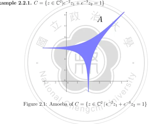
(9) 2.2. Tropical curves. For a complex plane curve C, we restrict it to the open subset (C∗ )2 of the (affine or projective) plane and then map it to the real plane by the map Log : (C∗ )2 → R2 z = (z1 , z2 ) 7→ (x1 , x2 ) := (log |z1 |, log |z2 |). The image A = Log(C ∩ (C∗ )2 ) is called the amoeba of the given curve C. Example 2.2.1. C = {z ∈ C2 |e−2 z1 + e−3 z2 = 1}. 立. 政治大. ‧. ‧ 國. 學 er. io. sit. y. Nat. al. n. i v −3 2 −2 n C Figure 2.1: Amoeba h of C = {z ∈ C | eU z1 + e z2 = 1} engchi In fact, the shape of the picture above (that also explains the name “amoeba”) can easily be explained. The curve C above contains exactly one point whose z1 -coordinate is zero, namely (0, e3 ). As log 0 = −∞, a small neighborhood of this point is mapped by Log to the tentacle of the amoeba A pointing to the left. Similarly, a neighborhood of (e2 , 0) is mapped by Log to the tentacle pointing down, and points of the form (z, e3 −ez) with |z| → ∞ to the tentacle pointing to the upper right.. 4.

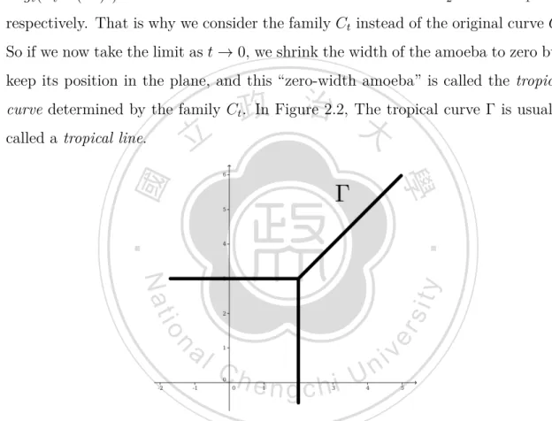
(10) Now, to make the amoeba into a combinatorial object, we consider the maps Logt : (C∗ )2 → R2. ( ) log |z1 | log |z2 | (z1 , z2 ) → 7 (− logt |z1 |, − logt |z2 |) = − ,− . log t log t. and the family of curves Ct = {z ∈ C2 | t2 z1 + t3 z2 = 1} for small t ∈ R. This family has the property that Ct passes through (0, t−3 ) and (t−2 , 0) for all t, and hence all Logt (Ct ∩ (C∗ )2 ) have their horizontal and vertical tentacles at z2 = 3 and z1 = 2, respectively. That is why we consider the family Ct instead of the original curve C. So if we now take the limit as t → 0, we shrink the width of the amoeba to zero but keep its position in the plane, and this “zero-width amoeba” is called the tropical. 政治大. curve determined by the family Ct . In Figure 2.2, The tropical curve Γ is usually. 立. called a tropical line.. ‧. ‧ 國. 學. n. er. io. sit. y. Nat. al. Ch. engchi. i Un. v. Figure 2.2: The tropical curve corresponding to the amoeba in Figure 2.1. There is an elegant way to hide the limiting process by replacing the ground field C by the field of Puiseux series. Definition 2.2.2. A formal power series of the form. ∑ q∈Q. (i) the set {q ∈ Q|aq ̸= 0} is bounded below,. 5. aq tq , aq ∈ C satisfying:.

(11) (ii) the denominators of q ∈ {q ∈ Q|aq ̸= 0} is a finite set is called a Puiseux series or a fractional power series. A field K of Puiseux series is a collection of Puiseux series. ∑ aq tq ∈ K, a ̸= 0, we may define the valuation of a Definition 2.2.3. For a = q∈Q. by the map val(a) = inf{q ∈ Q|aq ̸= 0}. Remark 2.2.4. The infimum of the set {q ∈ Q|aq ̸= 0} is actually a minimum. i.e. val(a) = inf{q ∈ Q|aq ̸= 0} = min{q ∈ Q|aq ̸= 0}. Example 2.2.5. Let. 政治大. a = 1 + t1/6 + t2/6 + t3/6 + . . . + tk/6 + . . . ,. 立. b = 1 + t1/2 + t1/3 + t1/4 + . . . + t1/k + . . . ,. ‧ 國. 學. and. c = 1 + t−1/6 + t−2/6 + t−3/6 + . . . + t−k/6 + . . . .. ‧. 1 1 1 1 a is a Puiseux series, while b and c is not, since the set of denominators of {0, , , , . . . , , . . .} 2 3 4 k 1 2 3 k is not finite, and {0, − , − , − , . . . , − , . . .} is not bounded below. 6 6 6 6. sit. y. Nat. er. io. It is easy to see that C ⊂ K, so we can consider a curve C in C2 to be a curve. al. n. iv n C 2 2 3 C = {z h ∈K = 1} e n| tgz1c+ht iz2 U. in K 2 , for example,. For t → 0, we have a ≈ aval a tval a . So applying the map logt to a, we get for a small t logt |a| ≈ logt |aval a tval a | = val a + logt |aval a | ≈ val a. Therefore, the process of applying the map Logt and taking the limit for t → 0 correspond to the map Val : (K ∗ )2 → Q2 (z1 , z2 ) 7→ (x1 , x2 ) := (−val z1 , −val z2 ). 6.

(12) Using this observation we can now give our first definition of plane tropical curves. Definition 2.2.6. A plane tropical curve is a subset of R2 of the form A = Val(C ∩ (K ∗ )2 ) , where C is a plane algebraic curve in K 2 . (Strictly speaking we should take the closure of Val(C ∩ (K ∗ )2 ) in R2 since the image of the valuation map Val is by definition contained in Q2 ) Note that this definition is now purely algebraic and does not involve any limit taking processes. Example 2.2.7. For the example above, C = {(z1 , z2 ) ∈ K 2 | t2 z1 + t3 z2 = 1}. If (z1 , z2 ) ∈ C ∩ (K ∗ )2 , then Val(z1 , z2 ) can give three kind of result:. 政治大 • If val z > −2, then the valuation of z = t − t z is −3 since all exponent 立 of t in t z are bigger then −3. Hence these points map precisely to the left 1. 2. −1. 1. 1. edge of the tropical curve determined by C.. 學. ‧ 國. −1. −3. ‧. • If val z2 > −3, then the valuation of z1 = t−2 − tz1 is −2 since all exponent of. Nat. sit. edge of the tropical curve determined by C.. y. t in tz1 are bigger then −2. Hence these points map precisely to the bottom. er. io. • If val z1 ≤ −2 and val z2 ≤ −3, then the equation t2 z1 + t3 z2 = 1 shows that. al. n. iv n C U edge of the tropical curve h etonthe This leads h i right g cupper. the leading terms of t2 z1 and t3 z2 must have the same valuation, i.e. that val z1 = val z2 + 1. determined by C.. So we can get the same graph by this definition. Let C ⊂ K 2 be a plane algebraic curve given by the polynomial equation { } ∑ C = (z1 , z2 ) ∈ K 2 | f (z1 , z2 ) := aij z1i z2j = 0 i,j∈N. for some aij ∈ K of which only finitely many are nonzero. Note that the valuation of a summand of f (z1 , z2 ) is val(aij z1i z2j ) = val aij + ival z1 + jval z2 . 7.

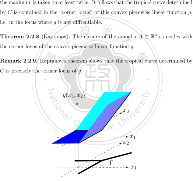
(13) Now if (z1 , z2 ) is a point of C then all these summands add up to zero. In particular, the lowest valuation of these summands must occur at least twice since otherwise the corresponding terms in the sum could not cancel. For the corresponding point (x1 , x2 ) = Val(z1 , z2 ) = (−val z1 , −val z2 ) of the tropical curve, this obviously means that in the expression g(x1 , x2 ) := max{ix1 + jx2 − val aij | (i, j) ∈ N2 with aij ̸= 0}. (2.1). the maximum is taken on at least twice. It follows that the tropical curve determined by C is contained in the “corner locus” of this convex piecewise linear function g, i.e. in the locus where g is not diffrentiable.. 政治大. Theorem 2.2.8 (Kapranov). The closure of the amoeba A ⊂ R2 coincides with. 立. the corner locus of the convex piecewise linear function g.. ‧ 國. 學. Remark 2.2.9. Kapranov’s theorem shows that the tropical curve determined by C is precisely the corner locus of g.. ‧. n. er. io. sit. y. Nat. al. Ch. engchi. i Un. v. Figure 2.3: A tropical curve as the corner locus of a convex piecewise linear function. 8.

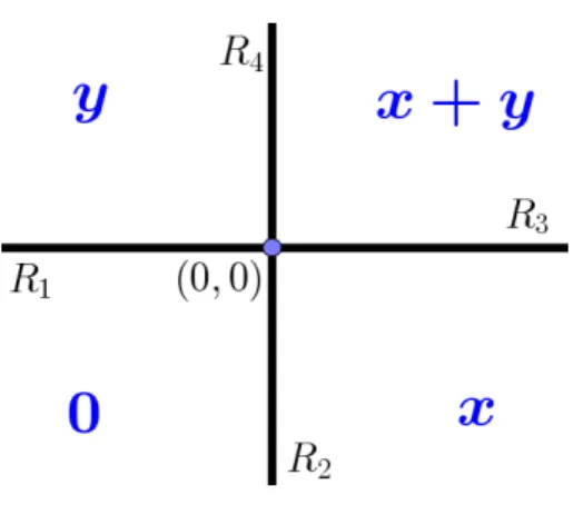
(14) Example 2.2.10. Let us consider the curve C = {z ∈ K 2 | t2 z1 + t3 z2 − 1 = 0} again. The corresponding convex piecewise linear function is g(x1 , x2 ) = max{x1 − 2, x2 − 3, 0} Figure 2.3 shows that the relation between tropical curve and the convex piecewise linear function g. Now, with the two tropical operations defined in Section 2.1, we can rewrite g as g(x1 , x2 ) = (−2) ⊙ x1 ⊕ (−3) ⊙ x2 ⊕ 0. 政治大. which is of the form of tropical polynomials.. 立. g(x1 , x2 ) =. ⊕. 學. ‧ 國. So we can also rewrite our convex piecewise linear function (2.1) above as ⊙j (−val aij ) ⊙ x⊙i 1 ⊙ x2. i,j∈N. ‧. Therefore, we can give an alternative definition of plane tropical curves that. sit. y. Nat. does not involve the somewhat complicated field of Puiseux series any more:. al. er. io. Definition 2.2.11. A plane tropical curve is a subset of R2 that is the corner locus. n. of a rational tropical polynomial.. Ch. engchi. i Un. v. From examples above, we may observe a simple proposition: Proposition 2.2.12. Suppose g(x1 , x2 ) = a ⊙ x ⊕ b ⊙ y ⊕ 0, where a, b ∈ Q, and let Γ be the corner locus of g. Then the coordinate of the vertex of Γ is (−a, −b). Remark 2.2.13. Let g(x1 , x2 ) =. ⊕. ⊙j aij ⊙ x⊙i 1 ⊙ x2 = max{ix1 +jx2 +aij | (i, j) ∈. i,j∈N. N2 , ai,j ∈ Q}. Each term of g(x1 , x2 ) corresponds to a plane g(x1 , x2 ) = ix+jy +aij .. 9.

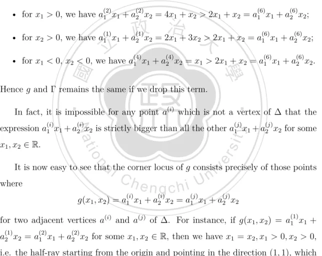
(15) Figure 2.4: The correspondence between coefficients and planes. Example 2.2.14. There is a special case of plane tropical curves. If the tropical. 政治大. polynomial g is the maximum of linear functions without constant terms, i.e. ⊕. (i). 立x (i). ⊙a1. x1. (i). ⊙a2 2. (i). (i). = max{a1 x1 + a2 x2 | i = 1, . . . , n}. (2.2). 學. ‧ 國. g(x1 , x2 ) =. i. (i). for some a(i) = (a1 , a2 ) ∈ N2 , then, since for each i, j = 1, . . . , n, i ̸= j, (i). (j). ‧. (i). (j). a1 x1 + a2 x2 = a1 x1 + a2 x2. y. Nat. er. io. sit. is a line passing through the origin, the corner locus of g is a cone. We have seen that a tropical curve is a graph in R2 whose edges are line seg-. n. al. Ch. i Un. v. ments. Let us consider Γ locally around a vertex V ∈ Γ. For simplicity we shift. engchi. coordinates so that V is the origin in R2 and thus Γ becomes a cone locally around V . Then Γ is locally the corner locus of a tropical polynomial of the form (2.2) Example 2.2.15. For convenient, we consider the tropical polynomial g(x1 , x2 ) = max{2x + 3y, 4x + y, 3x, x, 2y, 2x + y}. to be an example, and let a(1) = (2, 3), a(2) = (4, 1), a(3) = (3, 0), a(4) = (1, 0), a(5) = (0, 2), a(6) = (2, 1). Let ∆ be the convex hull of the points a(i) and Γ be the tropical curve of g. We may discover that a(6) is irrelevant for the tropical curve Γ, since. 10.

(16) Figure 2.5: A local picture of a tropical curve. (2). (2). (6). (6). • for x1 > 0, we have a1 x1 + a2 x2 = 4x1 + x2 > 2x1 + x2 = a1 x1 + a2 x2 ; (1). 政治大 (1). (6). (6). • for x2 > 0, we have a1 x1 + a2 x2 = 2x1 + 3x2 > 2x1 + x2 = a1 x1 + a2 x2 ;. 立. (4). (4). (6). (6). ‧ 國. 學. • for x1 < 0, x2 < 0, we have a1 x1 + a2 x2 = x1 > 2x1 + x2 = a1 x1 + a2 x2 . Hence g and Γ remains the same if we drop this term.. ‧. In fact, it is impossible for any point a(i) which is not a vertex of ∆ that the (i). (j). Nat. (i). (j). sit. n. al. er. io. x1 , x2 ∈ R.. y. expression a1 x1 + a2 x2 is strictly bigger than all the other a1 x1 + a2 x2 for some. i Un. v. It is now easy to see that the corner locus of g consists precisely of those points where g(x1 , x2 ) =. Ch. engchi. (i) a1 x 1. (i). (j). (j). + a2 x2 = a1 x1 + a2 x2 (1). for two adjacent vertices a(i) and a(j) of ∆. For instance, if g(x1 , x2 ) = a1 x1 + (1). (2). (2). a2 x2 = a1 x1 + a2 x2 for some x1 , x2 ∈ R, then we have x1 = x2 , x1 > 0, x2 > 0, i.e. the half-ray starting from the origin and pointing in the direction (1, 1), which is the outward normal of the edge joining a(1) and a(2) . By the same way, we will get the other four half-rays shown in Figure 2.5 on the right. The tropical curve Γ is simply the union of all these half-rays around V . Remark 2.2.16. In particular, all edges of Γ have rational slopes, since each a(i) is in N2 . 11.

(17) There is one more important condition on the edges of Γ around V , which is called the balancing condition. If a(1) , . . . , a(n) are the vertices of ∆ in clockwise direction, then an outward normal vector of the edge joining a(i) and a(i+1) (where we set a(n+1) := a(1) ) is (i). (i+1). v (i) := (a2 − a2. (i+1). , a1. (i). − a1 ) for i = 1, . . . , n. In particular, it follows that n ∑. v (i) = 0.. (2.3). i=1. Let u(i) be the primitive integral vector in the direction of v (i) and w(i) ∈ N>0 such that v (i) = w(i) · u(i) . We call w(i) the weight of the corresponding edge of Γ. Thus,. 政治大. we may consider Γ to be a weighted graph and rewrite (2.3) as. 立. n ∑. w(i) · u(i) = 0,. (2.4). i=1. ‧ 國. 學. which states that the weighted sum of the primitive integral vectors of the edges around every vertex of Γ is 0.. ‧. Example 2.2.17. Let us continue the Example 2.2.15. The edges of Γ pointing. Nat. sit. y. upper-right and pointing down have weight 2 (since v (1) = (2, 2) = 2 · (1, 1) and. al. n. balancing condition around the vertex V reads. Ch. engchi. er. io. v (3) = (0, −2) = 2 · (0, −1)), whereas all other edges have weight 1. Then the. i Un. v. 2 · (1, 1) + (1, −1) + 2 · (0, −1) + (−2, −1) + (−1, 2) = (0, 0) in this example. Remark 2.2.18. In this thesis, we will usually label the edges with their corresponding weights unless these weights are 1. Definition 2.2.19. The (toric) degree of a plane tropical curve Γ is a collection D of integral vectors such that: a positive multiple of an integral vector u ∈ D if and only if there exists an end (i.e. an unbounded edge) of Γ which is in the direction of u. In such case, we include mu into D, where m is the sum of multiplicities of all such ends.. 12.

(18) Example 2.2.20. Again in the Example 2.2.15, the degree of the plane tropical curve Γ is {2(1, 1), (1, −1), 2(0, −1), (−2, −1), (−1, 2)}. Definition 2.2.21. If the degree of a plane tropical curve Γ is {(−d, 0), (0, −d), (d, d)}, then Γ is called a plane tropical curve of degree d. Definition 2.2.22. A plane tropical curve of degree d is a weighted graph Γ in R2 such that (a) every (bounded) edge of Γ is a line segment with rational slope; (b) Γ has d ends each in the direction (−1, 0), (0, −1), (1, 1) (where an end of weight w counts w times);. 立. 政治大. (c) at every vertex V of Γ the balancing condition holds: the weighted sum of the. ‧ 國. 學. primitive integral vectors of the edges around V is zero.. ‧. Remark 2.2.23. Strictly speaking, we have only explained above why a plane tropical curve in the sense of Definition 2.2.11 gives rise to a curve in the sense. Nat. sit. y. of Definition 2.2.22. One can show that the converse holds as well; according to. er. io. Andreas Gathmann [1], a proof can be found in [3] or [7] chapter 5.. al. n. iv n C U h e nofgacgiven to find all types of plane tropical curves h i degree.. Remark 2.2.24. With this definition it has now become a combinatorial problem. In fact, the construction given in Example 2.2.15 globalizes well. Assume that Γ is the tropical curve given as the corner locus of the tropical polynomial (i). (i). g(x1 , x2 ) = max{a1 x1 + a2 x2 + b(i) | i = 1, . . . , n} If g is the tropicalization of a polynomial of degree d, then the a(i) are all integer points in the triangle ∆d := {(a1 , a2 ) ∈ N2 | a1 + a2 ≤ d}. Consider two terms i, j ∈ {1, . . . , n} with a(i) ̸= a(j) . If there is a point (x1 , x2 ) ∈ R2 such that (i). (i). (j). (j). g(x1 , x2 ) = a1 x1 + a2 x2 + b(i) = a1 x1 + a2 x2 + b(j) , 13.

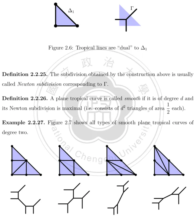
(19) then we draw a straight line in ∆d through the points a(i) and a(j) . In this way, we obtain a subdivision of ∆d whose edges correspond to the edges of Γ and whose 2-dimensional cells correspond to the vertices of Γ.. Figure 2.6: Tropical lines are “dual” to ∆1. 政治大 Definition 2.2.25. The subdivision 立 obtained by the construction above is usually. ‧ 國. 學. called Newton subdivision corresponding to Γ.. ‧. Definition 2.2.26. A plane tropical curve is called smooth if it is of degree d and 1 its Newton subdivision is maximal (i.e. consists of d2 triangles of area each). 2. y. sit. io. n. al. er. degree two.. Nat. Example 2.2.27. Figure 2.7 shows all types of smooth plane tropical curves of. Ch. engchi. i Un. v. Figure 2.7: The four types of (smooth) tropical plane conic. 14.

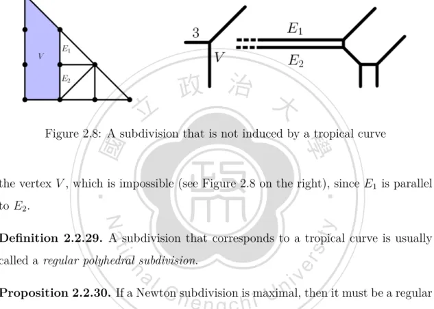
(20) Although it is a quite convenient way to draw a tropical curve by drawing its Newton subdivision first, there still have some problems. For example, not every subdivision gives rise to a type of tropical curves. Example 2.2.28. Here is an example of subdivisions that is not induced by a tropical curve. In Figure 2.8 on the left, we see that the edge E1 should meet E2 at. 立. 政治大. ‧ 國. 學. Figure 2.8: A subdivision that is not induced by a tropical curve. to E2 .. ‧. the vertex V , which is impossible (see Figure 2.8 on the right), since E1 is parallel. y. Nat. io. sit. Definition 2.2.29. A subdivision that corresponds to a tropical curve is usually. n. al. er. called a regular polyhedral subdivision.. Ch. i Un. v. Proposition 2.2.30. If a Newton subdivision is maximal, then it must be a regular polyhedral subdivision.. 2.3. engchi. Tropical factorization. Definition 2.3.1. Let g be a tropical polynomial. If a tropical curve Γ is a corner locus of g, then we say that Γ is a tropical curve of g, and denote it by T (g). Theorem 2.3.2. Let g1 , g2 be two tropical polynomials. We have T (g1 ⊙ g2 ) = T (g1 ) ∪ T (g2 ).. 15.

(21) i.e. The tropical curve of g1 ⊙ g2 is exactly the union of the tropical curves of g1 and g2 . In particular, the union of two plane tropical curves of degree d1 and d2 is always a plane tropical curve of degree d1 + d2 Example 2.3.3. Let g1 (x, y) = (−3)⊙x⊕(−1)⊙y⊕0 and g2 (x, y) = 1⊙x⊕1⊙y⊕0. We have g1 (x, y) ⊙ g2 (x, y) = (−2) ⊙ x⊙2 ⊕ (x ⊙ y) ⊕ y ⊙2 ⊕ 1 ⊙ x ⊕ 1 ⊙ y ⊕ 0. In Figure 2.9, we see that T (g1 ⊙ g2 ) is indeed the union of T (g1 ) and T (g2 ).. 立. 政治大. ‧. ‧ 國. 學 y. Nat. n. al. er. io. sit. Figure 2.9: T (g1 ⊙ g2 ) = T (g1 ) ∪ T (g2 ). Ch. i Un. v. Corollary 2.3.4. Let Γ be a tropical curve of degree ≥ 2. If Γ is an union of two. engchi. tropical curves Γ1 and Γ2 of degree lower than Γ, then there exists two tropical polynomials g1 and g2 with Γ1 = T (g1 ) and Γ2 = T (g2 ), resp, such that Γ = T (g1 ⊙ g2 ) Example 2.3.5. Let g(x, y) = x ⊕ y ⊕ 0. We now consider the tropical square of this polynomial g(x, y) ⊙ g(x, y) = x⊙2 ⊕ (x ⊙ y) ⊕ y ⊙2 ⊕ x ⊕ y ⊕ 0 = max{2x, x + y, 2y, x, y, 0}, then the tropical curve determined by this polynomial is still the same as g (but with weight 2). But as piecewise linear maps the function g(x, y) ⊙ g(x, y) is the 16.

(22) same as max{2x, 2y, 0} = x⊙2 ⊕ y ⊙2 ⊕ 0, and this tropical polynomial cannot be written as a product of two linear tropical polynomials. From Example 2.3.5, we know that the reducibility of tropical polynomials (of degree 2) and of plane tropical curves may not be the same. Definition 2.3.6. Two tropical polynomials are said to be equivalent(∼) if their tropical curves are the same.. 政治大. It is easy to see that this equivalence is an equivalence relation. Hence we may. 立. define the equivalence class of a tropical polynomial g with respect to ∼, and denote. ‧ 國. 學. it by g.. Now, we may introduce the definition of maximal coefficients of a tropical poly-. ‧. nomial.. y. Nat. sit. Definition 2.3.7. A coefficient aij of a tropical polynomial g(x, y) is a maximal. al. n. replacing aij with b is not equivalent to g(x, y).. Ch. engchi. er. io. coefficient if for any b ∈ Q with b > aij , the tropical polynomial h(x, y) formed by. i Un. v. Definition 2.3.8. A tropical polynomial is said to be maximally represented if all its coefficients are maximal coefficients. Remark 2.3.9. If g(x, y) is a tropical polynomial that T (g) is smooth, then g must be maximally represented. For any tropical polynomial g(x, y), the maximally represented polynomial of g may be unique, but not for the equivalence class g, see the following example. Example 2.3.10. Let us consider the following three polynomials: g1 (x, y) = 1 ⊙ x ⊕ 1 ⊙ y ⊕ 0, 17.

(23) g2 (x, y) = 6 ⊙ x ⊕ 6 ⊙ y ⊕ 5, and g3 (x, y) = 1 ⊙ x⊙2 ⊕ 1 ⊙ (x ⊙ y) ⊕ x. In Figure 2.10, we see that g1 , g2 and g3 are not the same piecewise linear functions, but with the same corner locus. Since tropical lines are smooth, these three polynomials are all the maximally represented polynomials.. 學. ‧ 國. 立. 政治大 Figure 2.10:. ‧. y. Nat. Although the maximally represented polynomials of g are not unique, we dis-. er. io. sit. cover the relation between them,. n. a l g2(x, y) = 5 ⊙ g1(x, y) i v n Ch U engchi. and. g3 (x, y) = x ⊙ g1 (x, y),. which would lead us to the following proposition. Proposition 2.3.11. Let g(x, y) be a tropical polynomial. Then we have T (g) = T (g ⊙ (a ⊙ x⊙b ⊙ y ⊙c )) where a ∈ Q, b, c ∈ N. With Proposition 2.3.11, we have the “uniqueness” of the maximally represented polynomial of g.. 18.

(24) Chapter 3. Recovering Tropical Polynomials from Tropical curves. 立. 政治大. ‧ 國. 學. In this chapter, we will introduce algorithms to recover the tropical polynomial from a given tropical curve.. ‧. Tropical curves of degree two. io. sit. y. Nat. 3.1. n. al. er. Theorem 3.1.1. Let Γ be a smooth plane tropical curve of degree two. Then Γ. i Un. v. can be represented as a corner locus of the tropical polynomial which is a product. Ch. engchi. of two linear tropical polynomials plus a certain tropical polynomial. Before the proof of Theorem 3.1.1, We first consider a tropical curve Γ locally around a vertex V ∈ Γ in the following two cases. Example 3.1.2. For convenience, we let g(x, y) = (−5) ⊙ x ⊕ (−4) ⊙ y ⊕ 0. If we add the coefficient of the constant term by −2, then we have h(x, y) := (−5) ⊙ x ⊕ (−4) ⊙ y ⊕ (−2) = (−2) ⊙ ((−3) ⊙ x ⊕ (−2) ⊙ y ⊕ 0) ∼ (−3) ⊙ x ⊕ (−2) ⊙ y ⊕ 0,. 19.

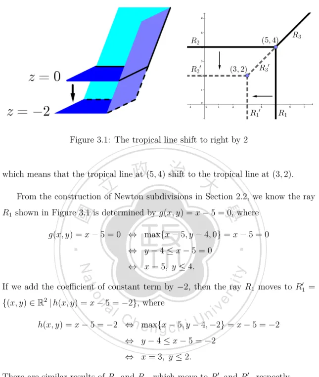
(25) Figure 3.1: The tropical line shift to right by 2. 政治大. which means that the tropical line at (5, 4) shift to the tropical line at (3, 2).. 立. From the construction of Newton subdivisions in Section 2.2, we know the ray. ‧ 國. 學. R1 shown in Figure 3.1 is determined by g(x, y) = x − 5 = 0, where g(x, y) = x − 5 = 0 ⇔ max{x − 5, y − 4, 0} = x − 5 = 0. ‧. ⇔ y−4≤x−5=0. y. sit. Nat. ⇔ x = 5, y ≤ 4.. er. io. If we add the coefficient of constant term by −2, then the ray R1 moves to R1′ =. al. {(x, y) ∈ R2 | h(x, y) = x − 5 = −2}, where. n. iv n C h(x, y) = x − 5 = −2 ⇔h e max{x 5, yi −U 4, −2} = x − 5 = −2 n g c− h ⇔ y − 4 ≤ x − 5 = −2 ⇔ x = 3, y ≤ 2.. There are similar results of R2 and R3 , which move to R2′ and R3′ , respectly. Example 3.1.3. Let g(x, y) = (x ⊙ y) ⊕ x ⊕ y ⊕ 0. The corresponding tropical curve is in Figure 3.2. (i). (i). Since a tropical curve T (g), for g(x, y) = max{a1 x + a2 y + b(i) | i = 1, . . . , n}, is the union of all these rays (i). (i). (j). (j). {(x, y) ∈ R2 | g(x, y) = a1 x + a2 y + b(i) = a1 x + a2 y + b(j) } 20.

(26) Figure 3.2: The tropical curve of g(x, y) = (x ⊙ y) ⊕ x ⊕ y ⊕ 0. where i, j = 1, . . . , n, i ̸= j. In this example, the rays is determined by these four. 政治大. planes: z = 0, z = x, z = y, and z = x+y. So if we add a negative number, e.g. −2,. 立. to the coefficient of constant term of g, we will have a similar result in Example 3.1.2. ‧ 國. 學. that the rays R1 and R2 move to R1′ and R2′ , respectly. Furthermore, we have a new edge E1 determined by h1 (x, y) = x = y, where h1 (x, y) := (x ⊙ y) ⊕ x ⊕ y ⊕ (−2).. ‧. Explicitly,. y. Nat. h1 (x, y) = x = y ⇔ max{x + y, x, y, −2} = x = y. n. al. ⇔ x = y, −2 ≤ x, y ≤ 0,. er. io. sit. ⇔ x + y ≤ x = y, −2 ≤ x = y. i Un. v. which implies the line segment E1 shown in Figure 3.3 on the left.. Ch. engchi. Now if we add a positive number, e.g. 3, to the coefficient of constant term of g, then we will have the result shown in Figure 3.3 on the right. The edge E2 is determined by h2 (x, y) = x + y = 3, where h2 (x, y) := (x ⊙ y) ⊕ x ⊕ y ⊕ 3. Explicitly, h2 (x, y) = x + y = 3 ⇔ max{x + y, x, y, 3} = x + y = 3 ⇔ x ≤ x + y = 3, y ≤ x + y = 3 ⇔ x + y = 3, 0 ≤ x, y ≤ 3, which implies the line segment E2 . Remark 3.1.4. One may observe that the “weight” of E1 is just the added number | − 2| = 2, where (0, 0) − (−2, −2) = (2, 2) = 2(1, 1). And the “weight” of E2 is just 21.

(27) Figure 3.3: The effect of adding numbers to the coefficient of constant term. the number 3, where (3, 0) − (0, 3) = (3, −3) = 3(1, −1).. 政治大 In Example 3.1.3, we show the effect on tropical curves that tuning a coefficient 立 of the corresponding tropical polynomials.. ‧ 國. 學. Let us beginning the proof of Theorem 3.1.1.. ‧. Proof of Theorem 3.1.1. Since there are just four types of smooth plane tropical. n. al. y. er. io. case 1.. sit. Nat. curves of degree two, we will prove this theorem by cases.. Ch. engchi. i Un. v. Figure 3.4:. (i). (i). Let Vi = (v1 , v2 ), i = 1, 2, 3, 4, and g be the corresponding tropical polynomial 22.

(28) of this tropical curve. In this case, we may observe that the local graphs around V1 , V3 , and V4 are locally tropical lines. If we “push” the vertex V4 to V2 (which actually means that adding a positive number to the coefficient of the x⊙2 -term of g so that such tropical line would shift to V2 ), the resulting curve would become an union of two tropical lines, i.e. the tropical line at V1 and the tropical line at V3 . The number we should add to x⊙2 -term of g is c1 = v1 − v1 (4). (2). in this case,. so that the vertex V4 would move to V2 , and the curve becomes the union of two tropical lines.. 政治大. 立. ‧. ‧ 國. 學. n. al. er. io. sit. y. Nat. Figure 3.5:. Ch. i Un. v. Conversely, if we substrct the x⊙2 -term of the tropical polynomial of this union. engchi. by c1 , then we will get the polynomial that corresponds to the original tropical curve. The polynomial of this union is (1). (1). (3). (3). G(x, y) := ((−v1 ) ⊙ x ⊕ (−v2 ) ⊙ y ⊕ 0) ⊙ ((−v1 ) ⊙ x ⊕ (−v2 ) ⊙ y ⊕ 0) = ((−v1 ) ⊙ (−v1 )) ⊙ x⊙2 ⊕ ((−v2 ) ⊙ (−v1 )) ⊙ (x ⊙ y) (1). (3). (1). (3). ⊕((−v2 ) ⊙ (−v2 )) ⊙ y ⊙2 ⊕ (−v1 ) ⊙ x ⊕ (−v2 ) ⊙ y ⊕ 0. (1). (3). (1). (1). Next, we do the substraction to the x⊙2 -term by adding the number to the other terms. For example, if we want to substract the x-term of 3 ⊙ x ⊕ 4 ⊙ y ⊕ 0 by 2,. 23.

(29) then due to the equivalence ∼, we may write the substraction as (3 ⊙ x ⊕ 4 ⊙ y ⊕ 0) ⊕ (6 ⊙ y ⊕ 2) = 3 ⊙ x ⊕ 6 ⊙ y ⊕ 2 = 2 ⊙ (1 ⊙ x ⊕ 4 ⊙ y ⊕ 0) ∼ 1 ⊙ x ⊕ 4 ⊙ y ⊕ 0. By this way, we add the coefficients of all the other terms but x⊙2 -term by c1 , then we have (1). (3). g(x, y) = G(x, y) ⊕ (((−v2 ) ⊙ (−v1 ) ⊙ c1 ) ⊙ (x ⊙ y) ⊕((−v2 ) ⊙ (−v2 ) ⊙ c1 ) ⊙ y ⊙2 (1). (3). (1). ⊕((−v1 ) ⊙ c1 ) ⊙ x. 政治大 (1). ⊕((−v2 ) ⊙ c1 ) ⊙ y ⊕ c1 ).. 立. case 2.. ‧. ‧ 國. 學. n. er. io. sit. y. Nat. al. Ch. engchi. i Un. v. Figure 3.6: (i). (i). Let Vi = (v1 , v2 ), i = 1, 2, 3, 4, and g be the corresponding tropical polynomial of this tropical curve. In this case, we may observe that the local graphs around V1 (3). (2). and V4 are locally tropical lines. From our experience, if we add c2 = v1 − v1 to the coefficient of x⊙2 -term of (1). (1). (4). (4). G(x, y) := ((−v1 ) ⊙ x ⊕ (−v2 ) ⊙ y ⊕ 0) ⊙ ((−v1 ) ⊙ x ⊕ (−v2 ) ⊙ y ⊕ 0) = ((−v1 ) ⊙ (−v1 )) ⊙ x⊙2 ⊕ ((−v2 ) ⊙ (−v1 )) ⊙ (x ⊙ y) (1). (4). (1). (4). ⊕((−v2 ) ⊙ (−v2 )) ⊙ y ⊙2 ⊕ (−v1 ) ⊙ x ⊕ (−v2 ) ⊙ y ⊕ 0, (1). (4). (1). 24. (1).

(30) then we will get the polynomial corresponding to the original tropical curve, i.e. g(x, y) = h(x, y) ⊕ (((−v1 ) ⊙ (−v1 ) ⊙ c2 ) ⊙ x⊙2 ). (1). (4). case 3.. 政治大. 立. ‧ 國. 學 ‧. (i). Figure 3.7:. (i). sit. y. Nat. Let Vi = (v1 , v2 ), i = 1, 2, 3, 4, and g be the corresponding tropical polynomial. io. al. er. of this tropical curve.. n. This case is similar to case 2. We first compute the polynomial of the union of. Ch. i Un. the tropical curve at V1 and the tropical curve at V4 , G(x, y) :=. (1) ((−v1 ). ⊙x⊕. engchi. (1) (−v2 ). v. (4). (4). ⊙ y ⊕ 0) ⊙ ((−v1 ) ⊙ x ⊕ (−v2 ) ⊙ y ⊕ 0). = ((−v1 ) ⊙ (−v1 )) ⊙ x⊙2 ⊕ ((−v1 ) ⊙ (−v2 )) ⊙ (x ⊙ y) (1). (4). (1). (4). ⊕((−v2 ) ⊙ (−v2 )) ⊙ y ⊙2 ⊕ (−v1 ) ⊙ x ⊕ (−v2 ) ⊙ y ⊕ 0. (1). (4). (1). (1). Second, we add c3 = v2 − v2 to the coefficient of the y ⊙2 -term of G(x, y), then (3). (2). we will have the desired polynomial g(x, y) = G(x, y) ⊕ (((−v2 ) ⊙ (−v2 ) ⊙ c3 ) ⊙ y ⊙2 ). (1). case 4.. 25. (4).

(31) Figure 3.8: (i). 政治大. (i). Let Vi = (v1 , v2 ), i = 1, 2, 3, 4, and g be the corresponding tropical polynomial. 立. of this tropical curve.. ‧ 國. 學. This case is also similar to case 2. We first compute the polynomial of the union of the tropical curve at V1 and the tropical curve at V4 , (1). ‧. (1). (4). (4). G(x, y) := ((−v1 ) ⊙ x ⊕ (−v2 ) ⊙ y ⊕ 0) ⊙ ((−v1 ) ⊙ x ⊕ (−v2 ) ⊙ y ⊕ 0) = ((−v1 ) ⊙ (−v1 )) ⊙ x⊙2 ⊕ ((−v1 ) ⊙ (−v2 )) ⊙ (x ⊙ y) (4). y. (1). sit. (4). Nat. (1). ⊕((−v2 ) ⊙ (−v2 )) ⊙ y ⊙2 ⊕ (−v1 ) ⊙ x ⊕ (−v2 ) ⊙ y ⊕ 0. (1). (4). (1). io. er. (4). a l(2) to the coefficient of thei vconstant term of G(x, y), n Ch U then we will have the desired polynomial engchi (3). n. Second, we add c4 = v1 − v1. g(x, y) = G(x, y) ⊕ c4 .. By these four cases, the proof is completed.. Algorithm 3.1.5. Here we give an algorithm to recover the polynomial of a given smooth plane tropical curve of degree two. Now, given a smooth plane tropical curve of degree two, denoted by Γ.. 26.

(32) 1. Choose two vertices V1 and V2 of Γ that are locally tropical lines, and let V3 and V4 be the last two vertices. 2. Compute the product of the polynomials of these two tropical lines, and denote it by G(x, y). 3. Let V5 be the intersection point of these two tropical lines. Let v1 be the vector from V5 to V3 , and v2 be the vector from V5 to V4 . Then we compute the vector v = v1 + v2 . 4. Write v = w · u, where u = (u1 , u2 ) is a primitive integral vector, and w is 1 1 a positive rational weight. For example, (−2, 0) = 2 · (−1, 0) and ( , ) = 2 2 1 · (1, 1). 2. 立. 政治大. 5. (1) If v = (−1, −1), then we substract the coefficient of constant term of. ‧ 國. 學. G(x, y) by w;. (2) if v = (1, 1), then we add the coefficient of constant term of G(x, y) by w;. ‧. (3) if v = (−1, 0), then we add the coefficient of x⊙2 -term of G(x, y) by w;. y. sit er. io. w;. Nat. (4) if v = (1, 0), then we substract the coefficient of x⊙2 -term of G(x, y) by. al. (5) if v = (0, −1), then we add the coefficient of y ⊙2 -term of G(x, y) by w;. n. iv n C h e n gthec h (6) if v = (0, 1), then we substract coefficient i U of y⊙2-term of G(x, y) by w; After these five steps, we will get the desired polynomial corresponding to Γ. Example 3.1.6. Given a plane tropical curve of degree 2 as in Figure 3.9. With some observations, we may discover that the graphs locally around (1, 1), (2, 5), and (4, 2) are tropical lines. Then we first compute the polynomial of the union of the tropical line at (1, 1) and the tropical line at (2, 5), i.e. h(x, y) := ((−1) ⊙ x ⊕ (−1) ⊙ y ⊕ 0) ⊙ ((−2) ⊙ x ⊕ (−5) ⊙ y ⊕ 0) = (−3) ⊙ x⊙2 ⊕ (−3) ⊙ x ⊙ y ⊕ (−6) ⊙ y ⊙2 ⊕ (−1) ⊙ x ⊕ (−1) ⊙ y ⊕ 0. 27.

(33) Figure 3.9: An example of smooth plane tropical curves of degree 2. 政治大 Next, the vector stated in Algorithm 3.1.5 is 立. ‧ 國. 學. v := [(2, 2) − (2, 2)] + [(4, 2) − (2, 2)] = (2, 0) = 2 · (1, 0). So, by Algorithm 3.1.5, we substract the coefficient of x⊙2 -term of h(x, y) by 2.. ‧. Thus, the desired polynomial is. Nat. io. sit. y. (−5) ⊙ x⊙2 ⊕ (−3) ⊙ x ⊙ y ⊕ (−6) ⊙ y ⊙2 ⊕ (−1) ⊙ x ⊕ (−1) ⊙ y ⊕ 0. n. al. er. Example 3.1.7. Given a plane tropical curve of degree 2 as in Figure 3.10.. Ch. engchi. i Un. v. Figure 3.10: An example of smooth plane tropical curves of degree 2. By the similar way in Example 3.1.6, we first compute the polynomial of the. 28.

(34) union of the tropical line at (−4, −4) and the tropical line at (12, 4), i.e. h(x, y) := (4 ⊙ x ⊕ 4 ⊙ y ⊕ 0) ⊙ ((−12) ⊙ x ⊕ (−4) ⊙ y ⊕ 0) = (−8) ⊙ x⊙2 ⊕ x ⊙ y ⊕ y ⊙2 ⊕ 4 ⊙ x ⊕ 4 ⊙ y ⊕ 0.. 立. 政治大. ‧ 國. 學. Figure 3.11: The union of T (4 ⊙ x ⊕ 4 ⊙ y ⊕ 0) and T ((−12) ⊙ x ⊕ (−4) ⊙ y ⊕ 0). ‧. Next, the vector stated in Algorithm 3.1.5 is. sit. y. Nat. v := [(0, 0) − (4, 4)] + [(8, 4) − (4, 4)] = (0, −4) = 4 · (0, −1).. al. n. the desired polynomial is. er. io. So, by Algorithm 3.1.5, we add the coefficient of y ⊙2 -term of h(x, y) by 4. Thus,. Ch. engchi. i Un. v. (−8) ⊙ x⊙2 ⊕ x ⊙ y ⊕ 4 ⊙ y ⊙2 ⊕ 4 ⊙ x ⊕ 4 ⊙ y ⊕ 0.. 3.2. Tropical curves of degree three. Definition 3.2.1. A maximal Newton subdivision of degree three is said to be normal if it is not one of the types shown in Figure 3.12. Proposition 3.2.2. Let ∆ be a Newton subdivision of degree three which is maximal. If ∆ is normal, then there must be a maximal Newton subdivision of degree two as a subgraph of ∆.. 29.

(35) Figure 3.12: The special four types. Proof. There are only the four types of Newton subdivisions shown in Figure 3.12 that does not have a maximal subdivision of degree two as a subgraph, we may check in Appendix A for all types of maximal subdivisions of degree three.. 政治大 Theorem 3.2.3. Let Γ be a smooth plane tropical curve of degree three. Then Γ 立 can be represented as a corner locus of the tropical polynomial which is a product. ‧ 國. 學. of three linear tropical polynomials plus a certain tropical polynomial.. ‧. We leave the proof to the end of Section 4.2.. y. Nat. Algorithm 3.2.4. Here we give an algorithm to recover the polynomial of a given. er. io. al. sit. smooth plane tropical curve of degree three.. n. Now, given a smooth plane tropical curve of degree three, denoted by Γ. Let ∆. Ch. be the Newton subdivision corresponding to Γ.. engchi. i Un. v. case 1. ∆ is normal. 1. Up to isomorphic, we may just consider the six types shown in Figure 3.13. 2. Let ∆2 be the subdivision of degree two which is a subgraph of ∆. Let ∆1 be a subdivision of degree one which is also a subgraph of ∆ but not a subgraph of ∆2 . Let Γ1 and Γ2 be the local graph of Γ corresponding to ∆1 and ∆2 , respectly. 3. Compute the corresponding polynomials of Γ1 and Γ2 , and then compute their product, we denote the product by G(x, y).. 30.

(36) 立. 政治大. ‧. ‧ 國. 學. n. 4. Let Vi =. (i) (i) (v1 , v2 ),. Figure 3.13:. Ch. engchi. er. io. sit. y. Nat. al. i Un. v. i = 1, 2, 3, 4. (2). (1). (4). (3). (1) For the first type in Figure 3.13, let c1 = v2 −v2 , and c2 = v2 −v2 . We add the coefficient of the y ⊙2 -term of G(x, y) by c1 , and add the coefficient of the y ⊙3 -term of G(x, y) by c1 − c2 . (2). (1). (4). (3). (2) For the second type, let c1 = v2 − v2 , and c2 = v2 − v2 . We add the coefficient of the y ⊙2 -term of G(x, y) by c1 , and add the coefficient of the y ⊙3 -term of G(x, y) by c1 + c2 . (2). (1). (4). (2). (3) For the third type, let c1 = v2 − v2 , and c2 = v2 − v2 . We add the. 31.

(37) coefficient of the y ⊙2 -term of G(x, y) by c1 , and add the coefficient of the y ⊙3 -term of G(x, y) by c1 + c2 . (2). (1). (4). (3). (4) For the forth type, let c1 = v2 − v2 , and c2 = v2 − v2 . We add the coefficient of the constant term of G(x, y) by c1 , and add the coefficient of the y ⊙3 -term of G(x, y) by c2 . (2). (1). (4). (3). (5) For the fifth type, let c1 = v2 −v2 , and c2 = v2 −v2 . We substract the coefficient of the constant term of G(x, y) by c1 , and add the coefficient of the y ⊙3 -term of G(x, y) by c2 . (2). (1). (4). (3). (6) For the sixth type, let c1 = v2 − v2 , and c2 = v2 − v2 . We substract. 治政 -term of G(x, y) by c 大 .. the coefficient of the constant term of G(x, y) by c1 , and substract the coefficient of the y. ⊙3. 立. 2. ‧ 國. 學. After these steps, we will get the desired polynomial corresponding to Γ. case 2. ∆ is not normal.. ‧. n. al. er. io. sit. y. Nat. 1. Up to isomorphic, we may just consider the two types shown in Figure 3.14.. Ch. engchi. Figure 3.14:. 32. i Un. v.

(38) 2. For the first type in Figure 3.14, (1) we observe that the graphs locally around V1 , V2 , and V3 are tropical lines. Let Γ1 , Γ2 , and Γ3 be the tropical lines whose vertices are at V1 , V2 , and V3 , respectly. (2) Find out the tropical polynomials of Γ1 , Γ2 , and Γ3 . Then, compute their product, and denote it by G(x, y). (2). (4). (2). (2). (9). (9). (3) Let c1 = v2 − v2 , c2 = v1 − v2 − v1 + v2 , and c3 = c1 + c2 + 1 (7) (8) (5) (v + v2 ) − v2 . Next, we add the coefficients of the y ⊙2 -term, the 2 2 x ⊙ y ⊙2 -term, and the y ⊙3 -term of G(x, y) by c1 , c2 , and c3 , respectly.. 政治大. And the resulting polynomial is the desired tropical polynomial.. 立. 3. For the second type in Figure 3.14,. ‧. ‧ 國. 學. 1 (5) (4) (7) (6) (8) (9) (1) let w1 = v2 − v2 , w2 = v2 − v2 , and w3 = v2 − v2 . Let c1 = (w1 + 2 1 1 w2 + w3 ) − w2 , c2 = (w1 + w2 + w3 ) − w3 , and c3 = (w1 + w2 + w3 ) − w1 . 2 2 (2) Let V1′ = (v1 +c1 , v2 ), V2′ = (v1 −c2 , v2 −c2 ), and V3′ = (v1 , v2 +c3 ). (1). (1). (2). (2). (3). (3). sit. y. Nat. Let g1 , g2 , and g3 be the tropical polynomials corresponding to the tropical. er. io. lines at V1′ , V2′ , and V3′ .. al. (3) Compute G(x, y) = g1 (x, y) ⊙ g2 (x, y) ⊙ g3 (x, y).. n. iv n C ⊙2 U (4) We add the coefficients of the y -term, and the x⊙2 ⊙ y-term hthe i e nx-term, h gc of G(x, y) by c1 , c2 , and c3 , respectly. And the resulting polynomial is the desired tropical polynomial. Example 3.2.5. Let us consider the curve in Figure 3.15: We see in Figure 3.16 that the corresponding subdivision is normal and is the forth type in Figure 3.13, so we compute the polynomials of Γ1 and Γ2 , and denote them by g1 and g2 , respectly. Next, we compute G(x, y) = g1 (x, y) ⊙ g2 (x, y). Since Γ1 is a tropical line at (−2, −2), we have g1 (x, y) = 2 ⊙ x ⊕ 2 ⊙ y ⊕ 0. 33.

(39) Figure 3.15:. 立. 政治大. ‧. ‧ 國. 學. n. By Algorithm 3.1.5, we have. Figure 3.16:. Ch. engchi. er. io. sit. y. Nat. al. i Un. v. 7 g2 (x, y) = (− ) ⊙ x⊙2 ⊕ (−3) ⊙ x ⊙ y ⊕ (−4) ⊙ y ⊙2 ⊕ (−1) ⊙ x ⊕ y ⊕ 0. 2 Next, we have the product G(x, y) = g1 (x, y) ⊙ g2 (x, y) 3 = (− ) ⊙ x⊙3 ⊕ (−1) ⊙ x⊙2 ⊙ y ⊕ (−1) ⊙ x ⊙ y ⊙2 ⊕ (−2) ⊙ y ⊙3 2 ⊕1 ⊙ x⊙2 ⊕ 2 ⊙ x ⊙ y ⊕ 2 ⊙ y ⊙2 ⊕ 2 ⊙ x ⊕ 2 ⊙ y ⊕ 0. Let c1 = 1 − 0 = 1 and c2 = 4 − 3 = 1. So we add the coefficients of constant term and the y ⊙3 -term of G(x, y) by c1 and c2 , respectly. Thus, we have the desired. 34.

(40) polynomial 3 (− ) ⊙ x⊙3 ⊕ (−1) ⊙ x⊙2 ⊙ y ⊕ (−1) ⊙ x ⊙ y ⊙2 ⊕ (−1) ⊙ y ⊙3 2 ⊕1 ⊙ x⊙2 ⊕ 2 ⊙ x ⊙ y ⊕ 2 ⊙ y ⊙2 ⊕ 2 ⊙ x ⊕ 2 ⊙ y ⊕ 1.. 立. 政治大. ‧. ‧ 國. 學. n. er. io. sit. y. Nat. al. Ch. engchi. 35. i Un. v.

(41) Chapter 4. Recovering Tropical Polynomials from Newton Subdivisions. 學. 4.1. ‧ 國. 立. 政治大. Newton subdivisions of degree two. ‧. Lemma 4.1.1. Each (maximal) Newton subdivision of degree two has two subdi-. n. al. er. io. sit. y. Nat. visions of degree one as subgraphs.. Ch. engchi. i Un. v. Figure 4.1: Four type of Newton subdivision of degree two. Theorem 4.1.2. For a Newton subdivision of degree two, there is a tropical polynomial corresponding to this subdivision, obtained by replacing a coefficient of a product of two tropical linear polynomials with a suitable number. Proof. For a maximal Newton subdivision of degree two, by Proposition 2.2.30,. 36.

(42) there is a tropical curve corresponding to this subdivision. Thus, by Theorem 3.1.1, there is a polynomial obtained by replacing a coefficient of a product of two tropical linear polynomials with a suitable number. Example 4.1.3. Let us consider the Newton subdivision of type 4 shown in Figure 4.1.. 立. 政治大. Figure 4.2: Type 4 of the Newton subdivision of degree two. ‧ 國. 學. In Figure 4.2, we see that the 1-cell V1 is at the upper right of V2 , since the. ‧. corresponding vertex of V1 is at the upper right of the corresponding vertex of V2 .. y. Nat. If the corresponding vertex of V1 is at (a1 , a2 ), and the corresponding vertex of V2. sit. is at (b1 , b2 ), we have a1 > b1 , a2 > b2 , and a2 − a1 > b2 − b1 . So we may suppose. al. n. linear polynomials is. er. io. (a1 , a2 ) = (4, 7) and (b1 , b2 ) = (0, 0) for example. The product of these tropical. Ch. engchi. i Un. v. ((−4) ⊙ x ⊕ (−7) ⊙ y ⊕ 0) ⊙ (x ⊕ y ⊕ 0). = (−4) ⊙ x⊙2 ⊕ (−4) ⊙ x ⊙ y ⊕ (−7) ⊙ y ⊙2 ⊕ x ⊕ y ⊕ 0. In Figure 4.3, the edge E is incident to the vertices corresponding to y-term and 2x-term, which means that E is determined by the coefficients of y-term and 2x-term. So we replace the coefficient of y, for instance, with 3. The resulting polynomial is (−4) ⊙ x⊙2 ⊕ (−4) ⊙ x ⊙ y ⊕ (−7) ⊙ y ⊙2 ⊕ x ⊕ 3 ⊙ y ⊕ 0, which is an example of tropical polynomials corresponding to Newton subdivisions of type 4.. 37.

(43) Figure 4.3: The edge E is determined by y-term and 2x-term. 4.2. 政治大. Newton subdivisions of degree three. 立. Theorem 4.2.1. For a normal subdivision ∆, there exist three tropical polynomials. ‧ 國. 學. g1 (x, y), g2 (x, y), and h(x, y), where g1 corresponds to a subdivision of degree one, ∆, such that g1 (x, y) ⊙ g2 (x, y) ⊕ h(x, y) corresponds to ∆.. Nat. sit. y. ‧. and g2 corresponds to a maximal subdivision of degree two that is a subgraph of. Proof. By Proposition 3.2.2, each normal subdivision has a maximal subdivision. io. n. al. er. of degree two as a subgraph, so up to isomorphic, we have six types shown in. i Un. v. Figure 4.4, where ∆2 is a maximal subdivision of degree two.. Ch. engchi. We see in Figure 4.4 that these six types can be obtained from the following two subdivisions shown in Figure 4.5. case 1. Let us start from the subdivision in Figure 4.5 on the left. Let g1 and g2 be the corresponding tropical polynomials of ∆1 and ∆2 , respectly. In Figure 4.6, we see that if we add a suitable number c1 to the coefficient of y ⊙2 -term of the tropical polynomial G1 (x, y) := g1 (x, y) ⊙ g2 (x, y), then we get a polynomial G2 which corresponds to the second case in Figure 4.6, where G2 (x, y) := G1 (x, y) ⊕ h1 (x, y), and h1 (x, y) is the tropical polynomial obtained by adding c1. 38.

(44) 政治大. Figure 4.4: Six types of maximal subdivisions of degree three. 立. y. ‧. ‧ 國. 學. Nat. er. io. sit. Figure 4.5:. al. iv n C c2 to the y ⊙3 -term of G2 , then we h will have a polynomial en g c h i U G3 which corresponds to n. to the coefficient of y ⊙2 -term of G1 . In the same way, if we add a siutable number. the third case in Figure 4.6, where G3 (x, y) := G2 (x, y) ⊕ h2 (x, y), and h2 (x, y) is the tropical polynomial obtained by adding c2 to the coefficient of y ⊙3 -term of G2 . On the other hand, if we add a siutable number c3 (which is larger than c2 ) to the y ⊙3 -term of G2 , then we will have a polynomial G4 which corresponds to the forth case in Figure 4.6, where G4 (x, y) := G2 (x, y) ⊕ h3 (x, y), and h3 (x, y) is the tropical polynomial obtained by adding c3 to the coefficient of y ⊙3 -term of G2 . In detail, suppose g1 (x, y) = a1 ⊙ x ⊕ a2 ⊙ y ⊕ 0. 39.

(45) Figure 4.6: The local graph of the corresponding subdivisions and. 立. 政治大. g2 (x, y) = b1 ⊙ x⊙2 ⊕ b2 ⊙ x ⊙ y ⊕ b3 ⊙ y ⊙2 ⊕ b4 ⊙ x ⊕ b5 ⊙ y ⊕ 0.. ‧ 國. 學. Then we have. G1 (x, y) = g1 (x, y) ⊙ g2 (x, y). ‧. = (a1 ⊙ b1 ) ⊙ x⊙3 ⊕ (a1 ⊙ b2 ⊕ a2 ⊙ b1 ) ⊙ x⊙2 ⊙ y. y. Nat. ⊕(a1 ⊙ b3 ⊕ a2 ⊙ b2 ) ⊙ x ⊙ y ⊙2 ⊕ (a2 ⊙ b3 ) ⊙ y ⊙3. io. sit. ⊕(a1 ⊙ b4 ⊕ b1 ) ⊙ x⊙2 ⊕ (a1 ⊙ b5 ⊕ a2 ⊙ b4 ⊕ b2 ) ⊙ x ⊙ y. er. ⊕(a2 ⊙ b5 ⊕ b3 ) ⊙ y ⊙2 ⊕ (a1 ⊕ b4 ) ⊙ x ⊕ (a2 ⊕ b5 ) ⊙ y ⊕ 0.. al. n. iv n C Choose 0 < c1 < a2 − b5 , and let ⊙ b5 ⊕ b3 ) ⊙ c1 ) ⊙ y ⊙2 . Then we h eh1(x, n gy)c=h((ai 2 U. have. G2 (x, y) = G1 (x, y) ⊕ h1 (x, y) = (a1 ⊙ b1 ) ⊙ x⊙3 ⊕ (a1 ⊙ b2 ⊕ a2 ⊙ b1 ) ⊙ x⊙2 ⊙ y ⊕(a1 ⊙ b3 ⊕ a2 ⊙ b2 ) ⊙ x ⊙ y ⊙2 ⊕ (a2 ⊙ b3 ) ⊙ y ⊙3 ⊕(a1 ⊙ b4 ⊕ b1 ) ⊙ x⊙2 ⊕ (a1 ⊙ b5 ⊕ a2 ⊙ b4 ⊕ b2 ) ⊙ x ⊙ y ⊕((a2 ⊙ b5 ⊕ b3 ) ⊙ c1 ) ⊙ y ⊙2 ⊕ (a1 ⊕ b4 ) ⊙ x ⊕ (a2 ⊕ b5 ) ⊙ y ⊕ 0. Let H1 (x, y) = h1 (x, y), then we have G2 (x, y) = G1 (x, y) ⊕ H1 (x, y). Next, choose c1 < c2 < c1 + 2b5 − b3 . Let h2 (x, y) = ((a2 ⊙ b3 ) ⊙ c2 ) ⊙ y ⊙3 . 40.

(46) Then we have G3 (x, y) = G2 (x, y) ⊕ h2 (x, y) = G1 (x, y) ⊕ h1 (x, y) ⊕ h2 (x, y) = (a1 ⊙ b1 ) ⊙ x⊙3 ⊕ (a1 ⊙ b2 ⊕ a2 ⊙ b1 ) ⊙ x⊙2 ⊙ y ⊕(a1 ⊙ b3 ⊕ a2 ⊙ b2 ) ⊙ x ⊙ y ⊙2 ⊕ ((a2 ⊙ b3 ) ⊙ c2 ) ⊙ y ⊙3 ⊕(a1 ⊙ b4 ⊕ b1 ) ⊙ x⊙2 ⊕ (a1 ⊙ b5 ⊕ a2 ⊙ b4 ⊕ b2 ) ⊙ x ⊙ y ⊕((a2 ⊙ b5 ⊕ b3 ) ⊙ c1 ) ⊙ y ⊙2 ⊕ (a1 ⊕ b4 ) ⊙ x ⊕ (a2 ⊕ b5 ) ⊙ y ⊕ 0. Let H2 (x, y) = h1 (x, y) ⊕ h2 (x, y), then we have G3 (x, y) = G1 (x, y) ⊕ H2 (x, y). Again, we choose c1 + 2b5 − b3 < c3 < 2c1 + 2b5 − b3 , and let. 政治大. h3 (x, y) = ((a2 ⊙ b3 ) ⊙ c3 ) ⊙ y ⊙3 .. 學. Then we have. ‧ 國. 立. G4 (x, y) = G2 (x, y) ⊕ h3 (x, y). ‧. = G1 (x, y) ⊕ h1 (x, y) ⊕ h3 (x, y). = (a1 ⊙ b1 ) ⊙ x⊙3 ⊕ (a1 ⊙ b2 ⊕ a2 ⊙ b1 ) ⊙ x⊙2 ⊙ y. Nat. sit. y. ⊕(a1 ⊙ b3 ⊕ a2 ⊙ b2 ) ⊙ x ⊙ y ⊙2 ⊕ ((a2 ⊙ b3 ) ⊙ c3 ) ⊙ y ⊙3. al. er. io. ⊕(a1 ⊙ b4 ⊕ b1 ) ⊙ x⊙2 ⊕ (a1 ⊙ b5 ⊕ a2 ⊙ b4 ⊕ b2 ) ⊙ x ⊙ y. n. ⊕((a2 ⊙ b5 ⊕ b3 ) ⊙ c1 ) ⊙ y ⊙2 ⊕ (a1 ⊕ b4 ) ⊙ x ⊕ (a2 ⊕ b5 ) ⊙ y ⊕ 0.. Ch. engchi. i Un. v. Let H3 (x, y) = h1 (x, y) ⊕ h3 (x, y), then we have G4 (x, y) = G1 (x, y) ⊕ H3 (x, y). Thus, we complete the proof in this case. case 2. Now, let us consider the lower three cases in Figure 4.4. Let g1 and g2 be the corresponding tropical polynomials of ∆1 and ∆2 , respectly. In Figure 4.7, we see that the three cases can be obtained by tuning the coefficients of constant term and 3y-term of the tropical polynomial G1 (x, y) := g1 (x, y)⊙g2 (x, y). Suppose g1 (x, y) = a1 ⊙ x ⊕ a2 ⊙ y ⊕ 0. 41.

(47) 政治大. Figure 4.7: The local graph of the corresponding subdivisions. 立. and. ‧ 國. 學. g2 (x, y) = b1 ⊙ x⊙2 ⊕ b2 ⊙ x ⊙ y ⊕ b3 ⊙ y ⊙2 ⊕ b4 ⊙ x ⊕ b5 ⊙ y ⊕ 0,. ‧. then we have. y. Nat. G1 (x, y) = g1 (x, y) ⊙ g2 (x, y). sit. = (a1 ⊙ b1 ) ⊙ x⊙3 ⊕ (a1 ⊙ b2 ⊕ a2 ⊙ b1 ) ⊙ x⊙2 ⊙ y. er. io. ⊕(a1 ⊙ b3 ⊕ a2 ⊙ b2 ) ⊙ x ⊙ y ⊙2 ⊕ (a2 ⊙ b3 ) ⊙ y ⊙3. al. iv n C ⊙2 ⊕(a2 ⊙ b5 ⊕ b3 )h⊙ey ⊕ (a1 ⊕i b4U n g c h ) ⊙ x ⊕ (a2 ⊕ b5) ⊙ y ⊕ 0. n. ⊕(a1 ⊙ b4 ⊕ b1 ) ⊙ x⊙2 ⊕ (a1 ⊙ b5 ⊕ a2 ⊙ b4 ⊕ b2 ) ⊙ x ⊙ y. Now, we choose 0 < c1 < a2 + b5 − b3 and 0 < c2 < b5 − a2 . Let h1 (x, y) = ((a2 ⊙ b3 ) ⊙ c1 ) ⊙ y ⊙3 ⊕ c2 . Then we have G2 (x, y) := G1 (x, y) ⊕ h1 (x, y) = (a1 ⊙ b1 ) ⊙ x⊙3 ⊕ (a1 ⊙ b2 ⊕ a2 ⊙ b1 ) ⊙ x⊙2 ⊙ y ⊕(a1 ⊙ b3 ⊕ a2 ⊙ b2 ) ⊙ x ⊙ y ⊙2 ⊕ ((a2 ⊙ b3 ) ⊙ c1 ) ⊙ y ⊙3 ⊕(a1 ⊙ b4 ⊕ b1 ) ⊙ x⊙2 ⊕ (a1 ⊙ b5 ⊕ a2 ⊙ b4 ⊕ b2 ) ⊙ x ⊙ y ⊕(a2 ⊙ b5 ⊕ b3 ) ⊙ y ⊙2 ⊕ (a1 ⊕ b4 ) ⊙ x ⊕ (a2 ⊕ b5 ) ⊙ y ⊕ c2 , which corresponds to the second case in Figure 4.7.. 42.

(48) Next, choose c3 > 0 and the same c1 for convenience. Let h2 (x, y) = ((a1 ⊙ b1 ) ⊙ c3 ) ⊙ x⊙3 ⊕ ((a1 ⊙ b2 ⊕ a2 ⊙ b1 ) ⊙ c3 ) ⊙ x⊙2 ⊙ y ⊕((a1 ⊙ b3 ⊕ a2 ⊙ b2 ) ⊙ c3 ) ⊙ x ⊙ y ⊙2 ⊕ ((a2 ⊙ b3 ) ⊙ c1 ⊙ c3 ) ⊙ y ⊙3 ⊕((a1 ⊙ b4 ⊕ b1 ) ⊙ c3 ) ⊙ x⊙2 ⊕ ((a1 ⊙ b5 ⊕ a2 ⊙ b4 ⊕ b2 ) ⊙ c3 ) ⊙ x ⊙ y ⊕((a2 ⊙ b5 ⊕ b3 ) ⊙ c3 ) ⊙ y ⊙2 ⊕ ((a1 ⊕ b4 ) ⊙ c3 ) ⊙ x ⊕((a2 ⊕ b5 ) ⊙ c3 ) ⊙ y. Then we have G3 (x, y) := G1 (x, y) ⊕ h2 (x, y) = ((a1 ⊙ b1 ) ⊙ c3 ) ⊙ x⊙3 ⊕ ((a1 ⊙ b2 ⊕ a2 ⊙ b1 ) ⊙ c3 ) ⊙ x⊙2 ⊙ y. 治政 ⊕ b ) ⊙ c ) ⊙ x ⊕ ((a ⊙大 b ⊕a ⊙b ⊕b )⊙c )⊙x⊙y 立 ⊕ b ) ⊙ c ) ⊙ y ⊕ ((a ⊕ b ) ⊙ c ) ⊙ x. ⊕((a1 ⊙ b3 ⊕ a2 ⊙ b2 ) ⊙ c3 ) ⊙ x ⊙ y ⊙2 ⊕ ((a2 ⊙ b3 ) ⊙ c1 ⊙ c3 ) ⊙ y ⊙3 ⊕((a1 ⊙ b4 ⊕((a2 ⊙ b5. 1. 3. 3. 3. ⊙2. ⊙2. 1. 5. 1. 4. 2. 2. 3. 3. 學. ⊕((a2 ⊕ b5 ) ⊙ c3 ) ⊙ y ⊕ 0,. ‧ 國. 4. which corresponds to the third case in Figure 4.7.. Nat. y. ‧. Next, for convenience, we choose the same c3 , and let. sit. h3 (x, y) = ((a1 ⊙ b1 ) ⊙ c3 ) ⊙ x⊙3 ⊕ ((a1 ⊙ b2 ⊕ a2 ⊙ b1 ) ⊙ c3 ) ⊙ x⊙2 ⊙ y. al. er. io. ⊕((a1 ⊙ b3 ⊕ a2 ⊙ b2 ) ⊙ c3 ) ⊙ x ⊙ y ⊙2 ⊕ ((a1 ⊙ b4 ⊕ b1 ) ⊙ c3 ) ⊙ x⊙2. n. iv n C ⊕((a2 ⊙ b5 ⊕ b3 ) ⊙ ch ⊙ y ⊙2 ⊕ ((a1i ⊕U 3 )e n g c h b4) ⊙ c3) ⊙ x ⊕((a1 ⊙ b5 ⊕ a2 ⊙ b4 ⊕ b2 ) ⊙ c3 ) ⊙ x ⊙ y. ⊕((a2 ⊕ b5 ) ⊙ c3 ) ⊙ y. Then we have G4 (x, y) := G1 (x, y) ⊕ h3 (x, y). = ((a1 ⊙ b1 ) ⊙ c3 ) ⊙ x⊙3 ⊕ ((a1 ⊙ b2 ⊕ a2 ⊙ b1 ) ⊙ c3 ) ⊙ x⊙2 ⊙ y ⊕((a1 ⊙ b3 ⊕ a2 ⊙ b2 ) ⊙ c3 ) ⊙ x ⊙ y ⊙2 ⊕ (a2 ⊙ b3 ) ⊙ y ⊙3 ⊕((a1 ⊙ b4 ⊕ b1 ) ⊙ c3 ) ⊙ x⊙2 ⊕ ((a1 ⊙ b5 ⊕ a2 ⊙ b4 ⊕ b2 ) ⊙ c3 ) ⊙ x ⊙ y ⊕((a2 ⊙ b5 ⊕ b3 ) ⊙ c3 ) ⊙ y ⊙2 ⊕ ((a1 ⊕ b4 ) ⊙ c3 ) ⊙ x ⊕((a2 ⊕ b5 ) ⊙ c3 ) ⊙ y ⊕ 0. which corresponds to the last case in Figure 4.7, and we complete the proof.. 43.

(49) Figure 4.8:. Example 4.2.2. Let us consider the normal subdivision in the left of Figure 4.8.. 政治大. Use the algorithm in Section 4.1, we may suppose the tropical polynomial of ∆2 to be. 立. (x ⊕ (−4) ⊙ y ⊕ 0) ⊙ ((−4) ⊙ x ⊕ y ⊕ 0) ⊕ 1. ‧ 國. 學. = (−4) ⊙ x⊙2 ⊕ x ⊙ y ⊕ (−4) ⊙ y ⊙2 ⊕ x ⊕ y ⊕ 1,. and the tropical polynomial of ∆1 to be (−8) ⊙ x ⊕ (−8) ⊙ y ⊕ 0.. ‧. Then we have the product of ∆1 and ∆2 to be. Nat. n. al. er. io. ⊕(−4) ⊙ x⊙2 ⊕ x ⊙ y ⊕ (−4) ⊙ y ⊙2 ⊕ x ⊕ y ⊕ 1.. sit. y. (−12) ⊙ x⊙3 ⊕ (−8) ⊙ x⊙2 ⊙ y ⊕ (−8) ⊙ x ⊙ y ⊙2 ⊕ (−12) ⊙ y ⊙3. i Un. v. Next, we replace the coefficients of x⊙3 and y ⊙3 by −11, then we have the desired polynomial. Ch. engchi. (−11) ⊙ x⊙3 ⊕ (−8) ⊙ x⊙2 ⊙ y ⊕ (−8) ⊙ x ⊙ y ⊙2 ⊕ (−11) ⊙ y ⊙3 ⊕(−4) ⊙ x⊙2 ⊕ x ⊙ y ⊕ (−4) ⊙ y ⊙2 ⊕ x ⊕ y ⊕ 1.. 44.

(50) Now, let us start the proof of Theorem 3.2.3. Proof of Theorem 3.2.3. First, we prove the theorem for tropical curves which correspond to normal subdivisions. In the proof of Theorem 4.2.1, we know that there are six types for normal subdivisions, up to isomorphic. So we may just prove the theorem for these six types. Let us consider the following example first.. 立. 政治大. ‧. ‧ 國. 學 er. io. sit. y. Nat. Figure 4.9:. This curve is of the type shown in Figure 4.10. The right part of this curve is. n. al. Ch. i Un. v. just a smooth plane tropical curve of degree two, so we can use the algorithm in. engchi. Section 3.1 to find out its polynomial.. Figure 4.10:. For the left part of this curve, with a similar way in the proof of Theorem 4.2.1,. 45.

(51) we may first consider the case in Figure 4.11, and find out the polynomial of the curve shown in Figure 4.12. Next, we add the suitable numbers to the coefficients of y ⊙2 -term and y ⊙3 -term. Then we will get the polynomial corresponding to the original curve.. 治 Figure 4.11: 政大. 立. ‧. ‧ 國. 學 iv n U (6). n. al. er. io. sit. y. Nat Figure 4.12:. (i). Ch. (i). engchi. (6). Let Vi = (v1 , v2 ), i = 1, . . . , 9. Let g1 (x, y) = (−v1 ) ⊙ x ⊕ (−v2 ) ⊙ y ⊕ 0, (9). (9). (1). (1). g2 (x, y) = (−v1 ) ⊙ x ⊕ (−v2 ) ⊙ y ⊕ 0, g3 (x, y) = (−v1 ) ⊙ x ⊕ (−v2 ) ⊙ y ⊕ 0, (8). (7). and h1 (x, y) = c0 , where c0 = v1 − v1 . Then we have the polynomial of the right part to be G1 (x, y) := g1 (x, y) ⊙ g2 (x, y) ⊕ h1 (x, y) (9). (9). (6). (6). = ((−v1 ) ⊙ x ⊕ (−v2 ) ⊙ y ⊕ 0) ⊙ ((−v1 ) ⊙ x ⊕ (−v2 ) ⊙ y ⊕ 0) ⊕c0 = ((−v1 ) ⊙ (−v1 )) ⊙ x⊙2 ⊕ ((−v1 ) ⊙ (−v2 )) ⊙ (x ⊙ y) (6). (9). (6). (9). ⊕((−v2 ) ⊙ (−v2 )) ⊙ y ⊙2 ⊕ (−v1 ) ⊙ x ⊕ (−v2 ) ⊙ y ⊕ c0 . (6). (9). (6). 46. (9).

(52) (3). (2). (5). (4). Let c1 = v2 − v2 and c2 = v2 − v2 . Let h2 (x, y) = (((−v2 ) ⊙ (−v2 ) ⊕ (−v2 ) ⊙ (−v2 )) ⊙ c1 ) ⊙ y ⊙2 . (6). (9). (1). (9). Then we have G2 (x, y) := G1 (x, y) ⊙ g3 (x, y) ⊕ h2 (x, y), which is of the same type of the original curve. Next, we compare c1 and c2 . If c1 ≥ c2 , then we add the coefficient of y ⊙3 -term of G2 by c1 − c2 ; otherwise, we add all terms but y ⊙3 -term of G2 by c2 − c1 . We let h3 (x, y) to be this coefficient tuning polynomial.. 政治大. So we have that the polynomial of the original curve can be represented as. 立. G2 (x, y) ⊕ h3 (x, y). ‧ 國. 學. = (G1 (x, y) ⊙ g3 (x, y) ⊕ h2 (x, y)) ⊕ h3 (x, y). = (g1 (x, y) ⊙ g2 (x, y) ⊕ h1 (x, y)) ⊙ g3 (x, y) ⊕ h2 (x, y) ⊕ h3 (x, y). ‧. = g1 (x, y) ⊙ g2 (x, y) ⊙ g3 (x, y). sit. y. Nat. ⊕(h1 (x, y) ⊙ g3 (x, y) ⊕ h2 (x, y) ⊕ h3 (x, y)).. al. er. io. By this way, we may have similar results in other cases. We may find out the. n. polynomials of curves corresponding to ∆1 and ∆2 , and also their product, and. Ch. i Un. v. then use the algorithm in the proof of Theorem 4.2.1 to construct the polynomial of the original curve.. engchi. Now, let us consider the last four cases of which subdivision is not normal.. Figure 4.13: The special four types. In Figure 4.13, We see that the first type and the third type are isomorphic,. 47.

(53) while the second type and the forth type are isomorphic. So we may just consider the first two types. For the first type, we may observe that it can be obtained from the type shown in Figure 4.15 by adding a suitable number to the coefficient of the y ⊙3 -term. So this case is done.. 政治大. Figure 4.14: A special type of tropical curve. 立. ‧. ‧ 國. 學. n. Ch. engchi. er. io. sit. y. Nat. al. Figure 4.15:. i Un. v. For the second type, we may observe that it can be obtained from the union of three tropical lines shown in Figure 4.17 by adding suitable numbers to the coefficients of x-term, y ⊙2 -term, and (x⊙2 ⊙ y)-term. Let the weight of the edges E1 , E2 , and E3 to be w1 , w2 , and w3 , respectly. Suppose we add c1 , c2 , and c3 to the coefficients of x, y ⊙2 , and (x⊙2 ⊙ y)-term of the polynomial of the union shown in Figure 4.17 to obtain the original curve. Then we have.    c + c2 = w1 ,   1 c2 + c3 = w2 ,     c +c = w . 3 1 3. 48.

(54) Figure 4.16: A special type of tropical curve. 立. 政治大. ‧ 國. 學. Figure 4.17: The union of three tropical lines. n. (i). sit. io. al. er. Nat.  1   c1 = (w1 + w2 + w3 ) − w2 ,   2     1 c2 = (w1 + w2 + w3 ) − w3 ,  2        c3 = 1 (w1 + w2 + w3 ) − w1 . 2. y. ‧. Thus, we have. Ch. engchi. i Un. v. (i). Let Vi = (v1 , v2 ), i = 1, 2, 3. We have V1′ = (v1 + c1 , v2 ), (1). (1). V2′ = (v1 − c2 , v2 − c2 ), (2). (2). V3′ = (v1 , v2 + c3 ). (3). (3). Let g1 , g2 , and g3 be the tropical polynomials of the tropical lines at V1′ , V2′ , and V3′ , respectly. Suppose G1 (x, y) := g1 (x, y) ⊙ g2 (x, y) ⊙ g3 (x, y).. 49.

(55) For convenience, we let G1 (x, y) = a1 ⊙ x⊙3 ⊕ a2 ⊙ x⊙2 ⊙ y ⊕ a3 ⊙ x ⊙ y ⊙2 ⊕ a4 ⊙ y ⊙3 ⊕ a5 ⊙ x⊙2 ⊕a6 ⊙ x ⊙ y ⊕ a7 ⊙ y ⊙2 ⊕ a8 ⊙ x ⊕ a9 ⊙ y ⊕ 0. Then we have the polynomial of the original curve to be G2 (x, y) = a1 ⊙ x⊙3 ⊕ (a2 ⊙ c3 ) ⊙ x⊙2 ⊙ y ⊕ a3 ⊙ x ⊙ y ⊙2 ⊕ a4 ⊙ y ⊙3 ⊕ a5 ⊙ x⊙2 ⊕a6 ⊙ x ⊙ y ⊕ (a7 ⊙ c2 ) ⊙ y ⊙2 ⊕ (a8 ⊙ c1 ) ⊙ x ⊕ a9 ⊙ y ⊕ 0. It may also written as G2 (x, y) = G1 (x, y) ⊕ (h1 (x, y) ⊕ h2 (x, y) ⊕ h3 (x, y)),. 政治大. where h1 (x, y) is the tropical polynomial obtained by adding c1 to the coefficient. 立. of x-term of G1 ; h2 (x, y) is the tropical polynomial obtained by adding c2 to the. ‧ 國. 學. coefficient of y ⊙2 -term of G1 ; h3 (x, y) is the tropical polynomial obtained by adding c3 to the coefficient of (x⊙2 ⊙ y)-term of G1 .. ‧. Therefore, we complete the proof of Theorem 3.2.3.. n. er. io. sit. y. Nat. al. Ch. engchi. 50. i Un. v.

(56) Appendix A. All types of maximal Newton subdivisions of degree three. 立. 政治大. ‧. ‧ 國. 學. n. er. io. sit. y. Nat. al. Ch. engchi. 51. i Un. v.

(57) 立. 政治大. ‧. ‧ 國. 學. n. er. io. sit. y. Nat. al. Ch. engchi. 52. i Un. v.



(60) Bibliography. [1] Andreas Gathmann. Tropical algebraic geometry. Jahresber. Deutsch. Math.Verein., 108(1):3–32, 2006.. 政治大 Honor’s thesis, Brigham 立Young University, 2007.. [2] Nathan Grigg. Factorization of tropical polynomials in one and several variables.. ‧ 國. Acad. Sci. Paris, 336(8):629–634, 2003.. 學. [3] Grigory Mikhalkin. Counting curves via lattice paths in polygons. C. R. Math.. ‧. [4] Grigory Mikhalkin. Enumerative tropical algebraic geometry in R2 . J. Amer.. sit. y. Nat. Math. Soc., 18(2):313–377, 2005.. er. io. [5] Jürgen Richter-Gebert, Bernd Sturmfels, and Thorsten Theobald. First steps. al. n. iv n C volume 377 of Contemp. Math., Amer. Math. Soc., Providence, hpages e n g289–317. chi U. in tropical geometry. In Idempotent mathematics and mathematical physics,. RI, 2005.. [6] Imre Simon. Recognizable sets with multiplicities in the tropical semiring. In Michal Chytil, Ladislav Janiga, and Václav Koubek, editors, MFCS, volume 324 of Lecture Notes in Computer Science, pages 107–120. Springer, 1988. [7] David Speyer. Tropical geometry. PhD thesis, UC Berkeley, 2005. [8] Yen-Lung Tsai. Working with tropical meromorphic functions of one variable. Taiwanese J. Math., 16(2):691–712, 2012.. 55.

(61)