化學機械平坦化之最佳化操作：動態規劃法

全文

(1)國立交通大學機械工程研究所碩士論文. 化學機械平坦化之最佳化操作﹕ 動態規劃法 Optimal Operation of Chemical Mechanical Planarization﹕ Dynamic Programming Approach. 研究生:李永洲指導教授:林家瑞博士中華民國九十三年六月.

(2) 化學機械平坦化之最佳化操作：動態規劃法 Optimal Operation of Chemical Mechanical Planarization： Dynamic Programming Approach 研究生：李永洲. Student：Young-Chou Lee. 指導教授：林家瑞. Advisor：Dr. Chia-Shui Lin. 國立交通大學機械工程研究所碩士論文. A Thesis Submitted to Institute of Mechanical Engineering College of Engineering National Chiao-Tung University in Partial Fulfillment of the Requirements for the Degree of Master of Science In Mechanical Engineering June 2004 Hsinchu, Taiwan, Republic of China. 中華民國九十三年六月.

(3) 化學機械平坦化之最佳化操作：動態規劃法. 學生：李永洲. 指導教授：林家瑞. 博士. 國立交通大學機械工程研究所碩士論文. 摘要. 在本論文中，我們探討在一片二氧化矽或銅晶圓的研磨過程中，改變向下壓力與旋轉速度對不平坦度的影響。因為向下壓力與旋轉速度的大小皆有其限制的範圍，我們運用動態規劃設計有限向下壓力及旋轉速度的化學機械研磨之最佳化操作，並藉由更精確描述化學機械研磨的模型，在其他參數皆為固定的條件下，計算出輸入的改變量與時間，接著將最佳化計算結果在控片上作實驗，並與傳統的固定移除率操作方法作比較。此外，在有圖案的銅晶圓研磨，運用高處所受的向下壓力比低處高的假設，建立階梯高度的模型，並藉由模擬的結果說明向下壓力對平坦化效率的影響。. I.

(4) Optimal Operation of Chemical Mechanical Planarization： Dynamic Programming Approach. Student：Young-Chou Lee. Advisor：Dr. Chia-Shui Lin. Institute of Mechanical Engineering National Chiao Tung University. Abstract. In this thesis, the impact on non-planarization index by the down force and rotational speed during a SiO2 or Cu CMP process was investigated. Since the magnitudes of down force and rotational speed have limits, we choose the dynamic programming approach because of its ability to achieve constrained optimization by the down force and rotational speed. The duration and the amount of input were computed based on the more accurate chemical mechanical polishing model when the other parameters were fixed. Experiments based on dynamic programming were done for blanket wafers and the conventional operation was compared with the dynamic programming operation. Besides, the model for the step height reduction was established in the case of pattern wafer. The model was based on the assumption that at the feature scale, high areas on the wafer experience higher pressure than the lower areas. The influence of the planarization efficiency by the down force was discussed based on the simulation result. II.

(5) 誌謝. 感謝指導教授林家瑞博士兩年來細心與耐心的指導，讓我在碩士生涯中學習到如何做研究的方法，使我能掌握研究的方向，更重要的是學習到做人處世的原則。另外也感謝林仁輝博士與陳宗麟博士在論文口試時惠予的建議與指導，並感謝賴明志工程師對實驗上的協助，有各位的寶貴意見使我終於順利完成論文，非常感謝各位。在研究所的生活中，很幸運的能有建宇、朝雯、介民與木坤在一起打拼、一起打球、游泳與聊天，讓我的研究所生活增添許多樂趣，也更加充實與豐富，並感謝研究所認識的同學們，使生活充滿歡笑與快樂。最後，感謝家人的支持與鼓勵，使我無顧慮與專心的在學業上努力，也感謝女友的關心與包容。在此，僅將此論文獻給我最親愛的父母。. III.

(6) Contents Chinese Abstract……………………………………………………………………...I English Abstract……………………………………………………………………...II Acknowledgement…………………………………………………………………...III List of Tables………………………………………………………………………...VI List of Figures……………………………………………………………………..VIII Chapter 1 Introduction………………………………………………………………1 1.1 Literature Survey and Motivation………………………………………………1 1.2 Thesis Outline…………………………………………………………………..3 Chapter 2 An Overview of CMP Process and Model Representation…………….5 2.1 Introduction of CMP Structure……………………………………………….....5 2.2 CMP Process Parameters………………………………………………………..7 2.2.1 Mechanical Parameters……………………………………………………7 2.2.2 Chemical Parameters……………………………………………………...8 2.3 Model of Chemical Mechanical Polishing……………………………………..10 2.3.1 Preston Equation……………………………………………………….....11 2.3.2 Luo and Dornfeld Equation………………………………………………11 Chapter 3 Optimal Control Design：Dynamic Programming…………………....13 3.1 Bellman’s Principle of Optimality……………………………………………...13 3.2 Dynamic Programming………………………………………………………...14 3.3 Simulation Results……………………………………………………………...16 3.3.1 SiO2 CMP Process………………………………………………………..18 3.3.2 Cu CMP Process………………………………………………………….20 3.4 Discussion and Summary……………………………………………………....23 Chapter 4 Experiment and Discussion for SiO2 and Cu Blanket Wafer………....25 4.1 CMP Process for Experiment…………………………………………………..25 IV.

(7) 4.1.1 Sample Preparation……………………………………………………....25 4.1.2 Post CMP Cleaning……………………………………………………...26 4.1.3 Static Etching Experiment……………………………………………….26 4.2 Evaluation of CMP Performance……………………………………………....27 4.2.1 SiO2 and Cu Film Thickness Determination…………………………….27 4.2.2 CMP Removal Rate and Non-Planarization Index………………………27 4.3 SiO2 CMP Experiment………………………………………………………....28 4.3.1 Change Down Force as the Admissible Input…………………………...28 4.3.2 Change Rotational Speed as the Admissible Input………………………29 4.3.3 Change Down Force and Rotational Speed as the Admissible Inputs Simultaneously…………………………………………………………..29 4.4 Cu CMP Experiment…………………………………………………………...29 4.4.1 Change Down Force as the Admissible Input…………………………...30 4.4.2 Change Rotational Speed as the Admissible Input………………………30 4.4.3 Change Down Force and Rotational Speed as the Admissible Inputs Simultaneously………………………………………………………….31 4.5 Discussion and Summary……………………………………………………...31 Chapter 5 Pattern Copper Wafer………………………………………………….34 5.1 Introduction……………………………………………………………………34 5.2 Model development……………………………………………………………35 5.3 Simulation……………………………………………………………………..37 5.4 Discussion and Summary……………………………………………………...39 Chapter 6 Conclusion and Future Work…………………………………………..40 Reference…………………………………………………………………………….79. V.

(8) List of Tables Table 2-1 The Parameters of CMP Process………………………………………...41 Table 3-1 Process Parameters of SiO2 CMP Experiment…………………………..42 Table 3-2 Slurry Formulation of SiO2 CMP……………………………………….43 Table 3-3 The Experimental Results of SiO2 CMP to Determine C1 and C2………43 Table 3-4 The Experiment Data of SiO2 CMP……………………………………..43 Table 3-5 The Values of Admissible Inputs by Corresponding Down Force………43 Table 3-6 The Result of Dynamic Programming of SiO2 CMP with Down Force...44 Table 3-7 The Values of Admissible Inputs by Corresponding Rotational Speed …………………………………………………………………………..44 Table 3-8. The Result of Dynamic Programming of SiO2 CMP with Rotational Speed……………………………………………………………………44. Table 3-9 The Result of Dynamic Programming of SiO2 CMP with Two Inputs….44 Table 3-10 Process Parameters of Cu CMP Experiment…………………………...45 Table 3-11 Slurry Formulation of Cu CMP………………………………………...45 Table 3-12 The Experimental Results of Cu CMP to Determine C1 and C2……….46 Table 3-13 The Experiment Data of Cu CMP……………………………………...46 Table 3-14 The Values of Admissible Inputs by Corresponding Down Force…......46 Table 3-15 The Result of Dynamic Programming of Cu CMP with Down Force…46 Table 3-16 The Values of Admissible Inputs by Corresponding Rotational Speed …………………………………………………………………………47 Table 3-17 The Result of Dynamic Programming of Cu CMP with Rotational Speed …………………………………………………………………………47 Table 3-18 The Result of Dynamic Programming of Cu CMP with Two Inputs…..47. VI.

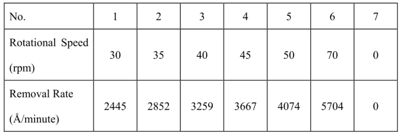
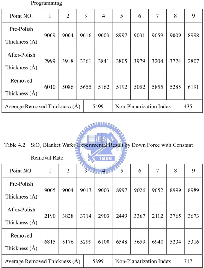
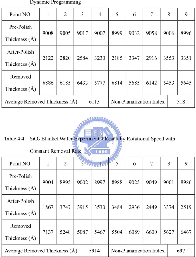
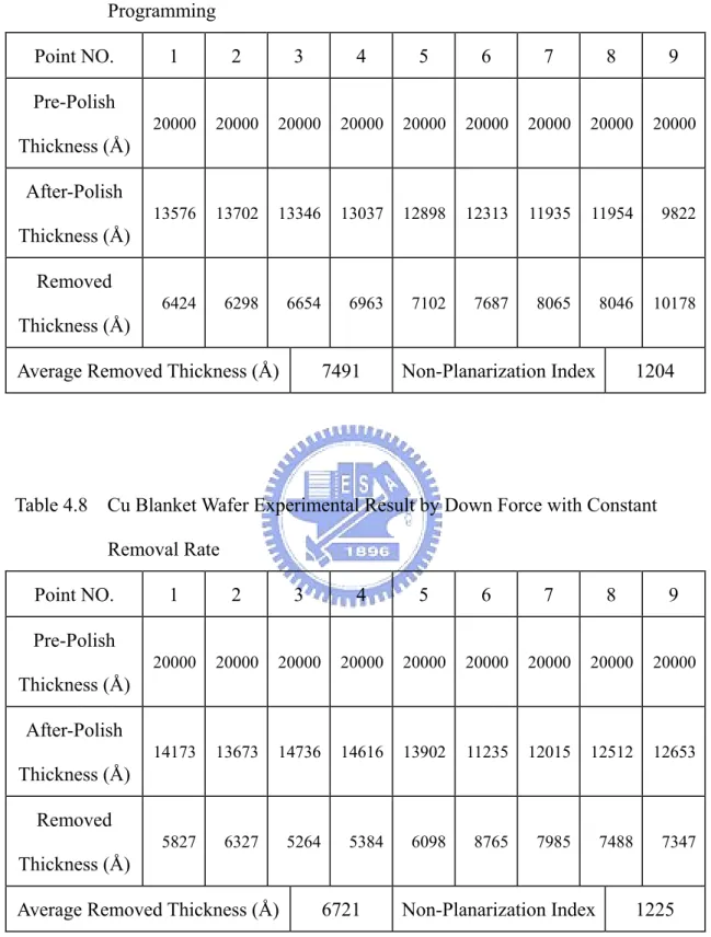
(9) Table 4.1 SiO2 Blanket Wafer Experimental Result by Down Force with Dynamic Programming…………………………………………………………….48 Table 4.2 SiO2 Blanket Wafer Experimental Result by Down Force with Constant Removal Rate……………………………………………………………48 Table 4.3 SiO2 Blanket Wafer Experimental Result by Rotational Speed with Dynamic Programming………………………………………………….49 Table 4.4 SiO2 Blanket Wafer Experimental Result by Rotational Speed with Constant Removal Rate………………………………………………….49 Table 4.5 SiO2 Blanket Wafer Experimental Result by Two Admissible Inputs with Dynamic Programming………………………………………………….50 Table 4.6 SiO2 Blanket Wafer Experimental Result by Two Admissible Inputs with Constant Removal Rate………………………………………………….50 Table 4.7 Cu Blanket Wafer Experimental Result by Down Force with Dynamic Programming…………………………………………………………….51 Table 4.8 Cu Blanket Wafer Experimental Result by Down Force with Constant Removal Rate……………………………………………………………51 Table 4.9 Cu Blanket Wafer Experimental Result by Rotational Speed with Dynamic Programming…………………………………………………………….52 Table 4.10 Cu Blanket Wafer Experimental Result by Rotational Speed with Constant Removal Rate………………………………………………...52 Table 4.11 Cu Blanket Wafer Experimental Result by Two Admissible Inputs with Dynamic Programming…………………………………………………53 Table 4.12 Cu Blanket Wafer Experimental Result by Two Admissible Inputs with Constant Removal Rate………………………………………………...53 Table 4.13 Comparison of Non-Planarization Index (SiO2 Blanket Wafer)………..54 Table 4.14 Comparison of Non-Planarization Index (Cu Blanket Wafer)………….54 VII.

(10) List of Figures Figure 1.1 Schematics of a Single Layer Cu Interconnect： (a) Before Polishing (b) Ideal Case After Polishing and (c) Real Case After Polishing………….55 Figure 1.2 (a) Dependence of Copper Dishing and Oxide Erosion on Platen Speed. Wafer Pressure was Kept Constant. [10]……………………………….56 Figure 1.2 (b) Dependence of Copper Dishing and Oxide Erosion on Wafer Pressure. Platen Speed was Held Constant. [10]………………………………….56 Figure 1.3 Trajectory for RRmax=9000 Å/min, umax=360000 Å/min2, Hsmall=2000 Å, and RRsmall=2000 Å/min [9]…………………………………………….57 Figure 2.1 The Mimic Schematic of CMP………………………………………….58 Figure 2.2 CMP Motion…………………………………………………………….58 Figure 2.3 The Perspective Front-View of CMP System- Westech 372M Machine …………………………………………………………………………..59 Figure 2.4 The Removal Rate Curves for Pad with Conditioning and without Conditioning [8]………………………………………………………...60 Figure 2.5 The Removal Rate Curve for Platen Speed [16]………………………..60 Figure 2.6 The Removal Rate Curve for Down Force [16]………………………...61 Figure 2.7 MRR as a Function of Abrasive Size Distribution and Abrasive Weight Concentration [11]……………………………………………………....61 Figure 2.8 Effects of Oxidizer Concentration on Removal Rate [12]……………...62 Figure 2.9 Two Contact Modes of CMP：(a) Hydro-Dynamic Contact Mode and (b) Solid-Solid Contact Mode [8]…………………………………………..62 Figure 3.1 Illustration of the Principle of Optimality………………………………63 Figure 3.2 Complete Result of Dynamic Programming and Recovery of the Optimal Trajectory from Initial State x(0)……………………………………….63. VIII.

(11) Figure 3.3 A Controller Based on Retrieving the Results of the Dynamic Programming Computation from Memory……………………………..64 Figure 3.4 Program Flowchart of Dynamic Programming…………………………65 Figure 3.5 The Model Prediction and Experimental Observations of the Effects of the Down Force and Rotational Speed for SiO2 Blanket Wafer………..66 Figure 3.6 The Simulation Result of SiO2 Blanket Wafer when the Down Force as the Variable Input……………………………………………………….67 Figure 3.7 The Simulation Result of SiO2 Blanket Wafer when the Rotational Speed as the Variable Input…………………………………………………….68 Figure 3.8 The Simulation Result of SiO2 Blanket Wafer when the Rotational Speed and Down Force as the Variable Inputs Simultaneously………………..69 Figure 3.9 The Model Prediction and Experimental Observations of the Effects of the Down Force and Rotational Speed for Cu Blanket Wafer………….70 Figure 3.10 The Simulation Result of Cu Blanket Wafer when the Down Force as the Variable Input……………………………………………………...71 Figure 3.11 The Simulation Result of Cu Blanket Wafer when the Rotational Speed as the Variable Input…………………………………………………...72 Figure 3.12 The Simulation Result of Cu Blanket Wafer when the Rotational Speed and Down Force as the Variable Inputs Simultaneously………………73 Figure 4.1 (a) The Structure of SiO2 Blanket Wafer (b) the Structure of Cu Blanket Wafer…………………………………………………………………...74 Figure 4.2 The Assembly of the Experiment for Static Etching [16]………………75 Figure 4.3 9 Points of Thickness Measurement……………………………………75 Figure 5.1 Typical Three-Step Procedure in Cu CMP: Planarization, Planarization/Overpolish, and Overpolish [28]………………………...76. IX.

(12) Figure 5.2 Schematic Picture of the Model………………………………………...76 Figure 5.3 Comparison between Luo and Dornfeld Equation and Power Function Fit for Experimental Cu Blanket Wafer Removal Rate…………………….77 Figure 5.4 Model Prediction Compared with Experimental Data from Stavreva [22] for Step Height versus Polishing Time………………………………….78 Figure 5.5 Planarization Efficiency versus Down Force…………………………...78. X.

(13) Chapter 1 Introduction. The chemical mechanical polishing (CMP) process removes material from the wafer surface through both physical friction and chemical etch. CMP has been shown to be the only technology capable of achieving planarization on the global scale in the integrated circuits (IC) industry. CMP was developed at IBMTM during the early 1980s. At that time, multilevel interconnect technology was being pushed to the limits of circuit density and performance. This technique which helps improve both photolithography and deposition process solved this problem. CMP produces excellent planarization across the wafer surface as well as lessening the effects of existing surface defects and has the benefit of repeatable process, compatible with all device types and generations. Therefore, many semiconductor manufactures have been developing CMP process with all their strength in order to get an advantageous position in the IC industry.. 1.1 Literature Survey and Motivation. The interlayer dielectric (ILD) film has surface ridges that reflect the underlying metal interconnection patterns. In deep submicron photolithography, on the other hand, the margin of depth of focus is reduced to a submicron range, and the submicron-height surface ridges cause local defects in the photoresist pattern. That is, interlayer dielectric planarization has become more critical as the number of metal stack layers has increased [1]. In addition, higher operating frequencies for IC chips lead to higher current densities in smaller features of interconnection. As a result, a 1.

(14) highly reliable metal line which allows high current density is necessary [2]. Copper has emerged as the optimal interconnect material because of its lower electrical resistivity and better resistance to electromigration compared to aluminum. Patterned Cu lines are produced by a damascene process. In the damascene process, the dielectric is patterned, followed by the barrier and metal deposition. The barrier becomes necessary when using Cu as an interconnect material to prevent the rapid diffusion of the Cu into the dielectric. The final step in this process is CMP that removes the excess metal and provides global planarization. Fig. 1.1 schematically shows a single layer Cu interconnect structure before and after CMP. Two key problems in Cu pattern wafer CMP, namely copper dishing and oxide erosion, generate surface non-planarity which gives rise to issues with integrating multiple layers of metal. Copper and oxide thinning results in increased RC delay leading to inferior device performance. Therefore, we focus on the experiments for SiO2 and Cu CMP. The most well known equation for modeling the CMP process is the Preston’s equation [3]. Preston’s equation reflects the influence of process parameters including down force and relative velocity. In the last several years, the revised Preston’s equations concentrated on different elements of CMP. For example, Zhang and Busnaina [4] proposed an equation taking into account the normal stress and shear stress acting on the contact area between abrasive particles and wafer surfaces. Tseng and Wang [5] showed that the removal rate is proportional to the terms P5/6 and V1/2. Zhao and Shi [6], [7] consider the effects of the pad hardness and the contact between wafer and pad. However, most of the models are quite rough. Luo and Dornfeld [8] assumed an indentation-sliding model for the penetration of the pad and included an empirical accommodation of chemical reaction at the wafer surface. Compared with experiment results, the model accurately predicts the removal rate. Therefore, we used 2.

(15) the model to predict the removal rate in the dynamic programming approach. Jian-Bin Chiu and Cheng-Ching Yu etc. [9] used the concept of soft landing of a spacecraft to CMP operation. Therefore, the CMP operation can be formulated as a minimum time optimal control problem. They treat the oxide surface as the landing surface, the polishing pad as a fly vehicle, and the removal rate as the vertical velocity. The equations describing the removal can be expressed as： & ⎤ ⎡0 − 1⎤ ⎡ H ⎤ ⎡0⎤ ⎡H ⎢& ⎥ = ⎢ ⎥ ⎢RR ⎥ + ⎢1⎥ u 0 0 R R ⎦⎣ ⎦ ⎣ ⎦ ⎣ ⎦ ⎣. − u max ≤ u ≤ u max where H is the thickness of material to be removed, RR the removal rate, and u the rate of change of the removal rate. The constraints in removal rate and rate of change of removal rate are applied because the parameters of CMP machine have physical limit, e.g. platen speed, down force, and slurry flow rate. They also set the final condition to H(tf) =2000Å and RR(tf) =2000 Å/min in order to reduce the dishing and erosion according to the experimental data proposed by K. Wijekoon and S. Tsai etc. [10]. Fig. 1.2 shows the dishing and erosion are proportional to the pressure and relative velocity. Once the landing point is reached (H(tf) =2000Å), the polisher continues the removal with the smaller removal (RR(tf) =2000 Å/min) until the end point is detected. Fig. 1.3 shows the result of optimal operation. Through their inspiration, we plan to use dynamic programming as our method of optimal operation in this thesis.. 1.2 Thesis Outline. In this study, we focus on the mechanical effects in CMP. The down force and rotational speed were taken to be the operational parameters. In chapter 2, an 3.

(16) overview of the CMP process and the parameters of mechanical and chemical aspects were introduced and the model which was used in simulation was represented. In chapter 3, the method of dynamic programming was introduced and the simulation data were discussed. In chapter 4, the experimental results through the operation of dynamic programming were obtained and the result was discussed. In chapter 5, we focus on the step height reduction by the down force based on the force redistribution. The simulation data were presented. Finally, the conclusion and future work were presented in chapter 6.. 4.

(17) Chapter 2 An Overview of CMP Process and Model Representation. CMP has been used to polish a variety of material for thousands of year, for example to produce optically flat and mirror finished surface. More recently optically flat and damage-free glass and semiconductor surfaces have been prepared by use of the CMP processes. Now CMP is being introduced in planarizing the interlayer dielectric and metal wiring to form interconnections between device and device.. 2.1 Introduction of CMP structure. A schematic of a CMP machine and the perspective front-view of a typical CMP system are shown in Fig. 2.1, 2.2 and 2.3. Both the carrier and pad are rotated in the same direction with different velocities. The flowing slurry is carried onto the wafer surface through the porosity on the pad surface. The slurry chemically attacks and softens the wafer surface, which is then removed by mechanical abrasion. The primary segments of CMP machine are as follows：. (1). Wafer Carrier： The wafer carrier holds the wafer face down during CMP and brings the wafer in contact with the polishing pad. The carrier rotates in the same direction as the platen.. (2). Platen： The rotating base on which the polishing pads are placed. Sometimes referred 5.

(18) to as the polishing “table”.. (3). Polish Arm： Transport the wafer by the polish arm.. (4). Pad： A pad which is mounted on a rotating platen and polishes the wafer. Polishing pads come in a variety of materials and are designed with a variety of surface features depending on the process results needed.. (5). Slurry： An abrasive mixture containing particles of colloidal silica, alumina, or some other abrasive material suspended in a chemical compound and DI water. Slurry is fed onto and through the polishing pad during CMP in order to remove material from the wafer surface.. (6). Pad Conditioning： A process in which the polishing pad is “roughed up” by a diamond disc in order to reduce the effects of glazing. In Fig. 2.4, conditioning enhances pad performance, but reduces overall pad lifetime.. If we only care about the amount of mechanical abrasion, it will result in a decreased removal rate and the wafer surface may peel off or be scratched. On the other hand, if we only care abut the amount of chemical reaction removal, it will lead to the erosion of the dielectric or the dishing of the metal lines. Giving undue emphasis to either of them will not achieve the global planarization. Therefore, how 6.

(19) to combine the mechanical abrasion and chemical reaction to get good performance and high throughput is nowadays an important challenge to be dealt with.. 2.2 CMP Process Parameters. As named chemical mechanical polishing, the primary parameters are divided into two parts which are the chemical aspect and the mechanical aspect.. 2.2.1 Mechanical Parameters. The primary mechanical parameters are as follows： (1) Platen Speed： The platen speed affects slurry transport across the wafer and the transport of the reactions and products of chemical reactions to and from the wafer surface. It has been noted that the copper removal rate is strongly dependent on the platen speed. In Fig. 2.5 [16], as the platen speed increases, the removal rate increases.. (2) Carrier Speed： When the carrier speed is the same as the platen speed, the best uniformity will be achieved.. (3) Down Force： In Fig. 2.6 [16], as the down force increases, the removal rate increases and then reduces the polishing time. This, of course, means higher throughput. The danger is that too much down force can cause problems such as scratches or gouges, and can possibly cause non-uniformity. 7.

(20) (4) Back Pressure： It is sometimes used to provide some curvature or shape to the wafer during polishing. The idea is to produce an optimum wafer shape with respect to the pad underneath for improving removal rate distribution on the wafer and within-wafer-uniformity (WIWUN).. (5) Pad Conditioning： There are variables which will affect pad conditioning. For instance, the conditioning duration, the abrasiveness of the disc and down force will all have an effect on the pad. A long conditioning duration may improve pad performance, but ultimately will reduce pad lifetime.. (6) Slurry Flow Rate： Slurry flow rate affects how quickly new chemicals and abrasive are delivered to the pad and reaction by-products and used abrasive are removed from pad. It also affects how much slurry is on the pad and therefore will affect the lubrication properties of the system.. Furthermore, there are still other mechanical parameters which affect the process：polish oscillation, wafer mounting and pad hardness, for instance.. 2.2.2 Chemical Parameters. The primary chemical parameters are as follows： (1) Abrasive Size Abrasive size affects the removal rate and the surface damage. For example, 8.

(21) experimental results show that there is an inverse proportional relationship between the abrasive size and the material removal rate, Fig. 2.7 [11].. (2) Abrasive Weight Concentration Abrasive weight concentration also affects the removal rate. For instance, experimental results show that there is a proportional relationship between the abrasive concentration and the material removal rate, Fig. 2.7 [11].. (3) Abrasive Variety Silica oxide (SiO2) is the most common used for oxide polishing while aluminum oxide (Al2O3) is the most common used for metal polishing.. (4) Slurry Viscosity The more viscous a material, the more it resists flow. High slurry viscosity results in poor transport of reactants and products to and from the wafer surface. It also affects lubrication of the wafer pad interface.. (5) Oxidizer Concentration In Fig. 2.8 [12], at the region of low oxidizer concentration, the rate of oxide generation is small and the passivation layer is removed as soon as it is formed. Then a maximal removal rate is reached when the rate of passivation is equal to the rate of mechanical abrasion. As we increase the oxide concentration further, the passivation itself changes its structure. This creates a barrier for mechanical abrasion and slows down the removal rate.. Furthermore, there are still other chemical parameters which affect the process： 9.

(22) slurry temperature, slurry buffering and film hardness, for instance. There are many variables that can affect the CMP performance as shown in Table 2-1. Besides, some factors which are difficult to control and monitor like the slurry transport under the wafer and the local temperature of the slurry also have significant effects on the CMP performance and the process parameters are interrelated such that modifications to one parameter will have an impact on other process issues. For instance, increasing platen speed or down force may increase the removal rate, yet at the same time create slurry flow rate and distribution problems. Therefore, the key problem is how to optimize the process parameter settings in order to obtain the desired results for the given film being planarized.. 2.3 Model of Chemical Mechanical Polishing. The material removal model for CMP can be separated into two parts, mechanical model and chemical model. The chemical action of the slurry is responsible for continuously softening the silicon oxide or oxidizing the metal surface to form a thin passive layer which is immediately removed by the action of the slurry abrasives. The fresh silicon oxide or metal surface exposed due to the abrasion is then rapidly repassivated and removed. This process of passivation-abrasion-repassivation continuous until the desired thickness is realized. Based on this idea, a mechanical removal model and a chemical model can be independently developed for CMP, with the mechanical model considering only the mechanical removal of the passivation layer, and the chemical model considering only the passivation of this layer.. 10.

(23) 2.3.1 Preston Equation. Preston provided a simple model of material removal in glass polishing tools, postulated based on experimental observation that the removal rate is proportional to the nominal applied pressure and the relative velocity between the pad and the material being polished. Preston equation [3] for the removal rate RR can be written as RR = Kp P V where P is the down pressure, V the relative velocity of wafer, and Kp a constant representing the effect of other remaining parameters, such as the abrasive type and concentration, and the nature of the chemicals and their concentrations. This equation has been widely used in CMP process control and consumable development for IC fabrication and manufacturing. However, it is focused on mechanical removal of material and there are some other phenomenons that can not be explained. For example, experimental results show that the pressure dependence of removal rate for CMP with soft pad satisfies a nonlinear relationship. Therefore, what is included in the all-purpose parameter Kp is unclear.. 2.3.2 Luo and Dornfeld Equation. Luo and Dornfeld proposed a model to describe the interactions between the wafer, pad, and abrasives, which are quite different from those in conventional polishing or lapping processes due to the small pad hardness and different size scales of the pad asperity and the polishing abrasives. They assumed the removal mechanism in the solid-solid contact mode instead of the hydro-dynamic mode, as shown in Fig. 2.9. Luo and Dornfeld equation [8] for the removal rate RR can be written as 11.

(24) 1 RR = C 2 ⎛⎜1 − Φ ⎡3 − C1P0 3 ⎤ ⎞⎟ P0 V + RR C ⎢⎣ ⎥⎦ ⎠ ⎝. where P0 is the down pressure V is the relative velocity of wafer C1 is a constant representing the effect of slurry abrasives (average size and size distribution), wafer and pad hardness, and pad roughness C2 is a constant representing the effect of slurry chemicals, slurry abrasives, wafer size, wafer density, wafer hardness, pad material, and pad roughness Φ is the normal cumulative distribution function which representing the probability density of active abrasives over the wafer-pad interface Φ(x ) =. 1 2π. ∫. x. e −(1 2 ) t dt 2. −∞. RRC is the material removal due to chemical etch The values, C1 and C2, are independent of the down force P0 and the relative velocity V. This model primarily is also focused on mechanical effect, particularly the abrasion due to the abrasive-wafer and abrasive-pad contact, but it includes the chemical reaction at the wafer surface. Therefore, this model looks more comprehensive to describe the CMP process. In SiO2 CMP process the material removal due to chemical etch, RRchemical etch, is small compared with the mechanical removal but the material removal due to chemical etch in Cu CMP process may need to be considered for more accurate results. Therefore, we ignored the chemical etch effect in the simulation of SiO2 CMP process and the removal rate can be written as RR = C 2 ⎛⎜1 − Φ ⎡3 − C1 P0 3 ⎤ ⎞⎟ P0 V ⎢⎣ ⎥⎦ ⎠ ⎝ 1. 12.

(25) Chapter 3 Optimal Control Design：Dynamic Programming. Sociological, economic, and physical pressures in all areas of modern life have generated an accelerated demand for high-level decision-making based upon limited information about the processes being controlled. In 1950s, a systematic and concerted mathematical study of such decision-making situations was initiated by Richard Bellman. This pioneering work was based upon the fundamental system-theoretic notion of feedback, i.e., that decision rules should be based upon the current (and perhaps past) states of the process under study. Bellman and his colleagues continued to develop the feedback decision-making concept under the name of “dynamic programming”. The majority of problems of true practical concern were computationally intractable due to the limited state of the computing art at that time. As time goes on, a combination of rapid progress in computer technology, coupled with the development of refined computational procedures, has made it practical for solving a wide variety of problems in economics, engineering, operations research, and mathematics, itself.. 3.1 Bellman’s Principle of Optimality. The fundamental concept of dynamic programming originated by Bellman is called the principle of optimality. This principle may conceptually be thought as follows: Given an optimal trajectory from point A to point C, the portion of the trajectory from any intermediate point B to point C must be the optimal trajectory from B to C. In Fig. 3.1, if the path Ⅰ-Ⅱ is the optimal path from A to C, then 13.

(26) according to the principle of optimality path Ⅱ is the optimal path from B to C. The proof by contradiction for this case is immediate: Assume that some other path, such as Ⅱ´, is the optimum path from B to C. Then, path Ⅰ-Ⅱ´ has less cost than path Ⅰ-Ⅱ. However, this contradicts the fact that Ⅰ-Ⅱ is the optimal path from A to C, and hence Ⅱ must be the optimal path from B to C.. 3.2 Dynamic Programming. Consider a quantized state x ∈ X, at stage (N-1). At this state, each of the admissible decisions u(m) ∈ U is applied. X = [x 1 x 2 ... x n -1 x n ] , U = [u 1 u 2 ... u M -1 u M ] For each of these decisions the cost at the current stage can be determined as (m) (m) L = L [x, u , N - 1]. (m = 1,2,..., M). Next, for each of these decisions the next state at stage N is determined from the system equation, x. (m). ( N ) = g [x, u. (m). , N - 1]. (m = 1,2,..., M). The next step is to compute the minimum cost at stage N for each of the states x(m). However, in general a particular state x(m) will not lie on one of the quantized states x ∈ X at which the optimal cost I(x, N) is defined. In fact, it may lie outside of the range of admissible states. In the latter case the decision is rejected as a candidate for the optimal decision for this state and stage. If a next state x(m) does fall within the range of allowable states, but not on a quantized value, then it is necessary to use some type of interpolation procedure to compute the minimum cost function at these points. Assume, then that the values of the minimum cost at the states x(m) can be 14.

(27) expressed as a function of the values of the optimal cost at quantized states x ∈ X. I[x (m ) , N] = P[x (m ) , N, I(x, N )] , all x ∈ X where I(x, N) = L(x, N) . If, as is often the case, no decision is made at k=N, the final. stage, and hence the cost function at N depends only on the final state, x(N). The total cost of applying decision u(m) at state x, stage (N-1), can then be written as. [. ] [. F (m) = L x, u (m ) , N - 1 + I x (m ) , N 1. ]. The minimization can be achieved by simply comparing the M quantities. According to the functional equation, the minimum value will be the minimum cost at state x, stage (N-1).. { [. ] [. min L x, u (m ) , N - 1 + I x (m ) , N I[x, N - 1] = (m ) u ∈U. ]}. (3.1). the optimal decision at this state and stage, uˆ [x, N - 1] , is the control u(m) for which the minimum in Eq. (3.1) is actually taken on. This procedure is repeated at each quantized state x∈X at stage (N-1). When this has been done, I(x, N-1) and uˆ [x, N - 1] are known for all x∈X. It is now possible to compute I(x, N-2) and uˆ [x, N - 2] for all x∈X based on knowledge of I(x, N-1). The general iterative procedure continues this process. Suppose that I(x, k+1) is known for all x∈X. Then I(x, k) and uˆ [x, k] are computed for all x∈X from. { [. ] [. ]}. min L x, u (m ) , k + I x (m ) , k + 1 I[x, k ] = (m ) u ∈U. (3.2). where x(m) is determined from x. (m). = g [x, u. (m). , k]. and where I(x(m), k+1) is computed by interpolation on the known values I(x, k+1) for all x ∈ X： I[x (m ) , k + 1] = P[x (m ) , k + 1, I(x, k + 1)] , all x ∈ X. 15.

(28) The optimal decision uˆ [x, k] is the decision for which Eq. (3.2) takes on the minimum. The iterative procedure begins by computing uˆ [x, N - 1] and I(x,N-1) from the given boundary conditions I(x, N), and it continues until uˆ [x,0] and I(x, 0) have been computed. The complete results of dynamic programming are shown in Fig. 3.2. At each state of stage, the optimal decision is written blow, and the minimum cost is written above. Finally, we can find the optimal sequence of decisions starting from the given x(0) and system equation. This is called the recovery procedure and these decisions are the input for our experiments. However, this is based on the system equation when we lack the measure of state. Our simulated results were done in this manner. If we could monitor the state and stage of the system, the dynamic programming solution, uˆ [x, k] , leads to a feedback control or decision policy configuration. One method of implementing this solution is to simply store all the values of uˆ [x, k] in memory, monitor the state and stage of the system, and look up the appropriate value of uˆ [x, k] as required. This type of implementation is attractive because the dynamic programming calculations can be done off-line, and the only operation that needs to be done during the decision interval is retrieval of the appropriate optimal decision. The system configuration is as shown in Fig. 3.3.. 3.3 Simulation Results. We used the very simple concept to get the equation for our simulation. The differential equation of the thickness being polished is equal to the removal rate and we made the removal rate to be the input. The equation is written as. dh h& = = −RR = −u dt 16.

(29) where h is the thickness, RR the removal rate, u the input. The discretized version using a sampling period of T is h (k + 1) = h (k ) − T × u (k ). (3.3). where k is the stage. We assumed that there were only 7 values of the input (include 0) because of restrictions on the Westech 372M CMP machine and the sampling period T here was fixed to 1. For each of these inputs the cost at the current stage can be determined as 1 (m) 1 2 L = qh (k ) + ru 2 (k ) 2 2. (m = 1,2,...,7). (3.4). and the cost at the final stage N also was determined as I(x, N) = L(x, N) =. 1 2 sh N 2. (3.5). where s is the weighting factor of final state, q the weighting factor of transient state, and r the weighting factor of input. Then we suppose a quantized state h∈H and a admissible inputs u(m) ∈U are applied. H=[6000 5999 5998…2 1 0] (jN=6001) U=[u(1) u(2) u(3) u(4) u(5) u(6) u(7)] (mN=7) We could get I(h,N-1) and uˆ [h, N - 1] for all h∈H by substituting Eq. 3.3, Eq. 3.4 and Eq. 3.5 into Eq. 3.2 which is presented in section 3.2. I[6000, N - 1] , I[5999, N - 1] ,K, I[1, N - 1] , I[0, N - 1] uˆ (6000, N - 1) , uˆ (5999, N - 1) ,K, uˆ (1, N - 1) , uˆ (0, N - 1). It is now possible to compute I(h, N-2) and uˆ [h, N - 2] for all h∈ H based on knowledge of I(h, N-1). The iterative procedure continues until uˆ [h,0] and I(h, 0) have been computed. The program flowchart is shown in Fig. 3.4 and the complete results of dynamic programming can be plotted like Fig. 3.2. Finally, we can find the optimal sequence of inputs starting from the given h(0) and Eq. 3.3 by means of the recovery procedure. 17.

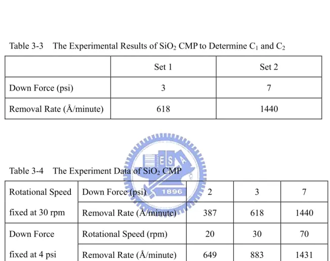
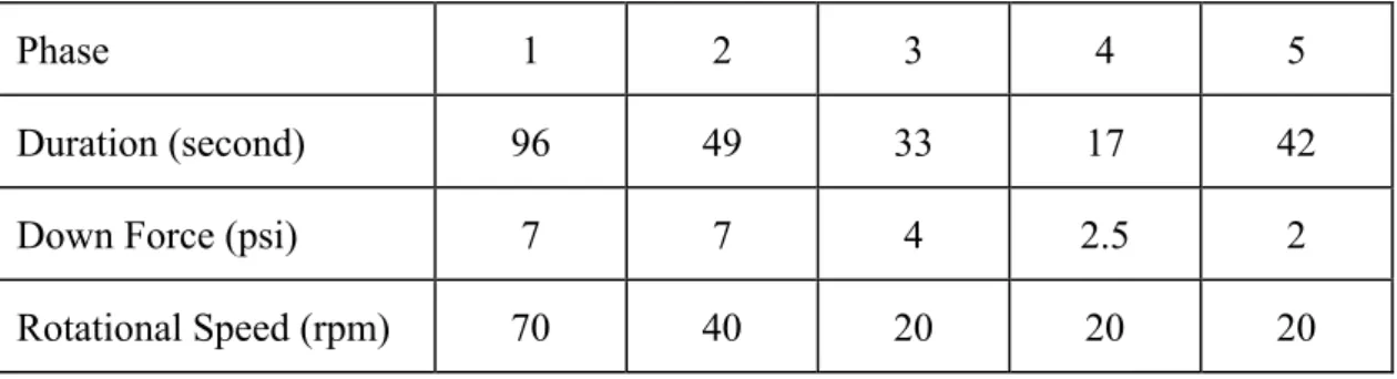
(30) 3.3.1 SiO2 CMP Process. Before we start to simulate dynamic programming, we have to determine the two constants, C1 and C2, in the Luo and Dornfeld equation. Furthermore, we modified the power of V from 1 to 6/10 which is based on Yin’s thesis [19] and the value of V means the rotational speed. Platen speed and carrier speed were all equal to the rotational speed. Two sets of experimental removal rate results are used to solve for the values of C1 and C2 by means of an iteration method of trial and error. The process parameters and slurry formulation used for SiO2 CMP experiment were listed in Table 3-1 and Table 3-2, and the two set of experimental results were listed in Table 3-3. The sample and evaluation of removal rate were mentioned in chapter 4. Then, we can solve for the values of C1 and C2 to be 8257 and 0.322, respectively. Thus, the removal rate prediction will be 1 (6 ) RR = 8257 ⎛⎜1 − Φ ⎡3 − 0.322 P0 3 ⎤ ⎞⎟ P0 V 10 . ⎥⎦ ⎠ ⎢⎣ ⎝. Table 3-4 shows the six experimental data of removal rate when the rotational speed is fixed at 30 rpm and the down force as the variable, and when the down force is fixed at 4 psi and the rotational speed as the variable. Fig. 3.5 shows the model prediction and experimental observations of the effects of the down force and rotational speed. Because C1 and C2 were based on the down force, the model prediction was better on the down force model than the rotational speed model. The error bars means the non-planarization index (the deviation of the removal rates of the nine points on the wafer). The smaller the non-planarization index, the more uniform removal rate on the entire wafer and it results in more flat surface. Decreasing the down force or rotational speed will decrease the non-planarization index. We try to reduce the down force or rotational speed after SiO2 film thickness is less than 2000 Å. 18.

(31) to get better non-planarization index. In order to reduce the down force or rotational speed when the thickness is less than 2000 Å we choose the weighting factors of final state, transient state and input to be 10000, 1 and 100000 respectively for the case of down force, and 10000, 1 and 700 for the case of rotational speed.. (a) Change down force as the admissible input to predict removal rate The 7 values of down force and the corresponding removal rates based on the Luo and Dornfeld equation were listed in Table 3-5 and these values were used as the admissible inputs for dynamic programming. The rotational speed was held at 30 rpm. The initial thickness h(0) was 6000 Å. Then, we started to simulate dynamic programming for optimal control of SiO2 CMP process and the result is shown in Fig. 3.6. According to the results, the process terminated at the 363th stage and the input is 7 psi during 0st~177th stage, 4 psi during 178th~225th stage, 2.5 psi during 226th~272th stage and 2 psi during 273th~362th stage. The data was tabulated in Table 3-6 and it was the basis of our SiO2 experiment on down force.. (b) Change rotational speed as the admissible input to predict removal rate The down force was held at 4 psi. The initial thickness h(0) is 6000 Å, we use the model that has been calculated above to predict removal rate as we change the rotational speed. Thus, the equation removal rate prediction is repeated here 1 (6 ) RR = 8257 ⎛⎜1 − Φ ⎡3 − 0.322 P0 3 ⎤ ⎞⎟ P0 V 10 . ⎥⎦ ⎠ ⎢⎣ ⎝. The 7 values of rotational speed and the corresponding removal rates based on the Luo and Dornfeld equation were listed in Table 3-7 and these values of removal rate were used as the admissible inputs for dynamic programming. Then,. 19.

(32) the result of dynamic programming is shown in Fig. 3.7. According to the results, the process terminated at the 334th stage and the input is 70 rpm during 0st~171th stage, 40 rpm during 172th~190th stage, 35 rpm during 191th~200th stage, 30 rpm during 201th~242th stage and 20 rpm during 243th~333th stage. The data was tabulated in Table 3-8 and it was the basis of our SiO2 experiment on rotational speed.. (c) Change down force and rotational speed as the admissible inputs simultaneously to predict removal rate At the beginning of the CMP process, we hoped that the removal rate was high enough to reduce the time of process and also obtained more flat surface at the end of the process. According to Dar’s thesis [16], the rotational speed has a great influence on the non-uniformity. For these reason we attempted to apply both inputs. We chose the weighting factors of final state, transient state, down force and rotational speed to be 10000, 1, 50000 and 1000 respectively. The result of dynamic programming is shown in Fig. 3.8. The rotational speed is decreased first in order to get better non-planarization index when the SiO2 film thickness is about 2000 Å and followed by the down force. The process terminated at the 237th stage. Certainly, the time was reduced compared to one admissible input. The data was tabulated in Table 3-9 and it was the basis of our SiO2 experiment on two sets of admissible inputs.. 3.3.2 Cu CMP Process. Two sets of experimental removal rate results are used to solve for the values of C1 and C2 as we did for the SiO2 CMP process. Furthermore, we adopted the original 20.

(33) power of V to 1 based on our experimental data. Platen speed and carrier speed were all equal to the rotational speed, V. The process parameters and slurry formulation used for Cu CMP experiment were listed in Table 3-10 and Table 3-11, and the two set of experimental results were listed in Table 3-12. The simulation of Cu CMP is similar to the SiO2 CMP and the only difference was that we had to consider the chemical etching rate in the Luo and Dornfeld equation. The chemical etching rate was obtained by experiment and the procedure was presented in chapter 4. The measured etching rate was about 14 Å/minute. It is quite small compared to the overall removal rate. The main reason was that we added a higher concentration of the citric acid. According to Ming’s thesis [17], as the concentration of citric acid in the HNO3-citric acid slurry increased, the etching rate of copper in the HNO3-citric acid slurry was suppressed. The citric acid behaves like BTA (Benzotriazole) in preventing copper corrosion in the HNO3-based solution. The BTA is a common Cu corrosion inhibitor since it can absorb on Cu surface to form a passivation layer. It is helpful to a Cu damascene structure because of the low etching rate at the recessed region of the Cu film. Furthermore, the removed thickness was only 6000 Å, hence we hoped that the removal rate was not too high. Therefore we omitted the chemical etching rate here. Then, we can solve for the values of C1 and C2 to be 30503 and 0.0113, respectively. Thus, the removal rate prediction will be 1 RR = 30503 ⎛⎜1 − Φ ⎡3 − 0.0113 P0 3 ⎤ ⎞⎟ P0 V ⎥⎦ ⎠ ⎢⎣ ⎝. (3.6). Table 3-13 shows the six experimental data of removal rate when the rotational speed is fixed at 30 rpm and the down force as the variable, and when the down force is fixed at 3.5 psi and the rotational speed as the variable. Fig. 3.9 shows the model prediction and experimental observations of the effects of the down force and rotational speed. The error bars means the non-planarization index (the deviation of. 21.

(34) the removal rates of the nine points on the wafer). In order to decreased the down force or rotational speed in the same manner of SiO2 when the Cu film thickness is less than 2000 Å we choose the weighting factors of final state, transient state and input to be 10000, 1 and 40000 respectively for the case of down force, and 10000, 1 and 1200 for the case of rotational speed.. (a) Change down force as the admissible input to predict removal rate The 7 values of down force and the corresponding removal rates based on the Luo and Dornfeld equation were listed in Table 3-14 and these values were used as the admissible inputs for dynamic programming. The rotational speed was held at 30 rpm. The initial thickness h(0) was 6000 Å. Then, we started to simulate dynamic programming for optimal control of Cu CMP process and the result is shown in Fig. 3.10. According to the results, the process terminated at the 118th stage and the input is 7 psi during 0st~67th stage, 5 psi during 68th~76th stage, 4 psi during 77th~84th stage, 3.5 psi during 85th~87th stage and 3 psi during 88th~117th stage. The data was tabulated in Table 3-15 and it was the basis of our Cu experiment on down force.. (b) Change rotational speed as the admissible input to predict removal rate The down force was held at 3.5 psi. The initial thickness h(0) is 6000 Å, we use the model that has been calculated above to predict removal rate as we change the rotational speed. Thus, the equation removal rate prediction is repeated here 1 RR = 30503 ⎛⎜1 − Φ ⎡3 − 0.0113 P0 3 ⎤ ⎞⎟ P0 V . ⎥⎦ ⎠ ⎢⎣ ⎝. The 7 values of rotational speed and the corresponding removal rates based on the Luo and Dornfeld equation were listed in Table 3-16 and these values of. 22.

(35) removal rate were used as the admissible inputs for dynamic programming. Then, the result of dynamic programming is shown in Fig. 3.11. According to the results, the process terminated at the 85th stage and the input is 70 rpm during 0st~40th stage, 50 rpm during 41th~47th stage, 45 rpm during 48th~50th stage, 35 rpm during 51th~57th stage and 30 rpm during 58th~84th stage. The data was tabulated in Table 3-17 and it was the basis of our Cu experiment on rotational speed.. (c) Change down force and rotational speed as the admissible inputs simultaneously to predict removal rate As we know that dishing and erosion are proportional to the pressure and rotational speed, we expected that decreasing the down force and rotational speed would improve the defects and also obtained better non-planarization index at the end of the process. Nevertheless only the blanket wafer of Cu was experimented since we lacked for pattern wafers. We chose the weighting factors of final state, transient state, down force and rotational speed to be 10000, 1, 20000 and 1200 respectively. The result of dynamic programming is shown in Fig. 3.12. The rotational speed is decreased first in order to get better non-planarization index when the Cu film thickness is about 2000 Å and followed by the down force. The process terminated at the 60th stage. Certainly, the time was reduced compared to one admissible input. The data was tabulated in Table 3-18 and it was the basis of our blanket Cu experiment on two sets of admissible inputs.. 3.4 Discussion and Summary. The Westech 372M machine in National Nano Device Laboratories (NDL) has 23.

(36) six phases to polish a wafer and each phase can be set some important parameters, like down force, platen speed and slurry flow rate, etc.. In order to operate in co-ordination with the CMP machine we could only have 7 values of the admissible input (include 0) and the method of dynamic programming has the advantage of dealing with the constrained inputs. The power of V in the Luo and Dornfeld equation was different between SiO2 and Cu because of the curve fitting of experimental data. The power of V for SiO2 and Cu were 6/10 and 1, respectively. The weighting factor of final state means the degree of final state that we want to be. The weighting factor of transient state means the speed of approaching to the final state. The last weighting factor, admissible input, means the degree of energy that we care about. In this thesis, we only want the admissible input to decrease when the thickness of SiO2 or Cu film is less than 2000 Å. In other words, the values of these weighting factors were determined by an iteration method of trial and error. In this chapter, three simulations of CMP operation include down force, rotational speed and both down force and rotational speed were examined. The simulated results of SiO2 and Cu CMP process revealed that the values of admissible inputs decreased regardless of operating down force or platen speed after the thickness was less than 2000 Å. Finally, we decreased the down force and rotational speed both. We made the rotational speed decrease first in order to get better non-planarization index and then decreased the down force to reduce the removal rate. This kind of operation also reduced the duration of polishing and enhanced the throughput simultaneously.. 24.

(37) Chapter 4 Experiment and Discussion for SiO2 and Cu Blanket Wafer. The experiments were carried out on the IPEC 372M CMP polisher. All polishing samples were prepared on p-type, (100)-oriented, 6-inch (150 mm) diameter silicon wafers.. 4.1 CMP Process for Experiment. 4.1.1 Sample Preparation. The thermally grown silicon dioxide film was obtained by wet oxidation (ASM/LB45 furnace system), in which the silicon was exposed to an ambient of H2 and O2 at 980˚C. The sample for the SiO2 CMP experiment was SiO2 film grown to 9000 Å thickness by this furnace system.. Si( s ) + 2 H 2 O( g ) ⎯⎯→ SiO2 ( s ) + 2 H 2( g ) ∆ The sample for the blanket Cu CMP experiment is a two-layer structure of Cu/Ta with thickness of 20000/500 Å sputter deposited by ULVAC SBH-3308 RDE sputter system on the silicon wafer which is covered with a 1000 Å thick thermally grown SiO2. The under layer of 500 Å Ta is used as an adhesion promoter for the copper deposition since copper itself does not adhere well on the thermal oxide. The structures of SiO2 and blanket Cu CMP wafer are shown in Fig. 4.1.. 25.

(38) 4.1.2 Post CMP Cleaning. Typically post-CMP cleaning is accomplished by a combination of methods, including wet chemical cleaning, megasonic cleaning, and mechanical polyvinyl alcohol (PVA) brush scrubbing. After polishing, post-CMP cleaning returns the wafer surface to an acceptable cleanliness level. Cleaning equipment must be able to remove slurry particle, heavy surface metals, and mobile ions without leaving macroscopic, microscopic, or electrically active defects is very important in making the process useful. Removal of particles from wafer surfaces requires the application of an external force that overcomes the force of adhesion. In this work, van der Waals and electrostatic double layer interactions are considered to be the adhesion forces. CMP slurry and post chemical cleans should not introduce any chemical or particulate contamination. Thus, cleaning processes must be designed for specific materials surface. The current technology of choice for Cu and SiO2 CMP cleaning uses one-side brush scrubbing. The experiments of this thesis use by the post-CMP cleaner of Solid State Equipment Corporation.. 4.1.3 Static Etching Experiment. Fig. 4.2 shows the assembly of the experiment for static etching. Because the slurry was not refreshed, we put a magnet at the bottom of the container to produce the flow of the slurry in order to keep the reaction rate at the surface stable. It also dispersed the abrasive to suspend in the slurry and made the experiment be closed to the real circumstance of polishing. The surface of Cu faced with the magnet and kept a distance with the magnet. The slurry formulation was tabulated in Table 3.11. We set the time to immerse the wafer in the slurry to 5 minutes and assumed that the 26.

(39) concentration of the slurry was constant during static etching.. 4.2 Evaluation of CMP Performance. 4.2.1 SiO2 and Cu Film Thickness Determination. The thicknesses of silicon dioxide thin films before and after polish process were measured by n&k analyzer thickness measurement system. The silicon dioxide film thickness was measured at 9 points, as shown in Fig. 4.3. To determine the thickness of copper film before and after CMP and static etching experiments, contact four point probe were used to measure the sheet resistance of copper film. Thickness of metal films is calculated by t=. ρ ρs. where t is the thickness of the metal film, ρ is the resistivity of the metal and ρs is the measured sheet resistance. Sheet resistance is measured at 9 points on the entire wafer in the same manner on SiO2 and we assume the copper resistivity is unchanged after CMP and static etching experiments.. 4.2.2 CMP Removal Rate and Non-Planarization Index. The CMP removal rates were monitored at 9 points along two perpendicular diameters on the entire wafer and are calculated by following formula： Removal Rate =. (Pre - CMP Thinkness ) − (Post - CMP Thinkness ) Polish Time. 27.

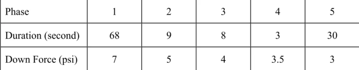
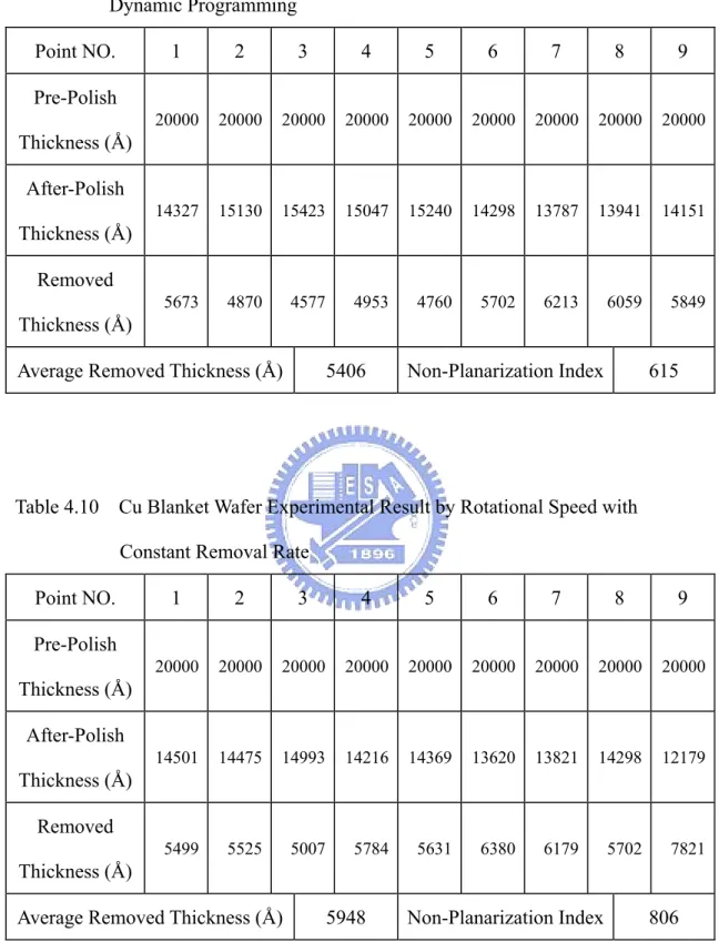
(40) The chemical etch rate is defined as： Chemical Etch Rate =. (Pre - Etch Thinkness ) − (Post - Etch Thinkness ) Chemical Etch Time. The within-wafer non-planarization index is defined as： 1 2 ⎞2 ⎛ 1 n Non - Planarization Index = ⎜ ∑ x −x ⎟ ⎟ ⎜ n − 1 i=1 i ⎠ ⎝. (. ). where x is the removed thickness (Å).. 4.3 SiO2 CMP Experiment. The experiments with dynamic programming were compared with the experiments which removed the same thickness at the same duration of polishing with constant removal rate. Since the removed thickness and duration of polishing were known, we can compute the value of constant removal rate. The parameters for the constant removal rate were found through the experiment.. 4.3.1 Change Down Force as the Admissible Input. The duration of polishing was 363 seconds and the removed thickness was 6000 Å. The required removal rate was 992 Å/minute. Because of the fixed rotational speed here, the required removal rate was found by changing the down force to be 4.3 psi. From the experimental results which were listed in Table 4.1 and 4.2, the constant removal rate operation mode has the better thickness removal but the dynamic programming operation mode possesses 39% better non-planarization index. The model prediction error on the lower down force caused the inaccuracy of thickness removal. It could be improved by developing more accurate model.. 28.

(41) 4.3.2 Change Rotational Speed as the Admissible Input. The duration of polishing was 334 seconds and the removed thickness was 6000 Å. The required removal rate was 1078 Å/minute. Because of the fixed down force here, the required removal rate was found by changing the rotational speed to be 40 rpm. Table 4.3 and 4.4 revealed the similar phenomenon to the part of down force. The dynamic programming operation mode possesses 26% better non-planarization index. The thickness removal was over 6000 Å for dynamic programming because the model prediction was lower than the experimental data on the higher rotational speed.. 4.3.3 Change Down Force and Rotational Speed as the Admissible Inputs Simultaneously. The duration of polishing was 237 seconds and the removed thickness was 6000 Å. The required removal rate was 1519 Å/minute. In order to avoid one-sided emphasis of these two inputs, we simultaneously increased the down force and rotational speed. The final value was found to be 4.7 psi and 52 rpm, respectively. The experimental results were listed in Table 4.5 and 4.6. The thickness removal had a little improvement and this might be caused by complementary model prediction. Nevertheless, the dynamic programming operation still possessed 16% better non-planarization index.. 4.4 Cu CMP Experiment. The same comparison between dynamic programming and constant removal rate were discussed as we did for the SiO2 CMP experiment. The parameters for the 29.

(42) constant removal rate were also found through the experiment.. 4.4.1 Change Down Force as the Admissible Input. The duration of polishing was 118 seconds and the removed thickness was 6000 Å. The required removal rate was 3051 Å/minute. Because of the fixed rotational speed here, the required removal rate was found by changing the down force to be 5.1 psi. From the experimental results which were listed in Table 4.7 and 4.8, the constant removal rate has the better thickness removal but the dynamic programming possesses a little better non-planarization index. However, the difference of non-planarization index between dynamic programming and constant removal rate is very small and it may be considered within statistical error of experimental data. It also shows that the down force is not a major factor to influence the non-planarization index in Cu CMP. As shown in Fig. 3.9, we see that the non-planarization index data under 3 psi and 5 psi is within statistical error with each other. This explains why there is no degradation in non-planarization index when the down force is decreased from 5.1 psi to 3 psi, i.e. there is no degradation in non-planarization index when Cu CMP process is changed from constant removal rate operation mode to dynamic programming operation mode. The inaccuracy of removed thickness may be caused by the lower predicted value of removal rate on the smaller down force. It means that the model for Cu CMP process needs to be modified.. 4.4.2 Change Rotational Speed as the Admissible Input. The duration of polishing was 85 seconds and the removed thickness was 6000 Å. The required removal rate was 4235 Å/minute. Because of the fixed down force here, 30.

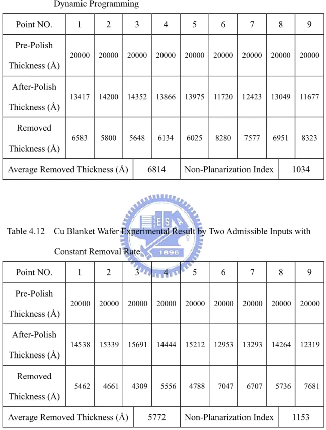
(43) the required removal rate was found by changing the rotational speed to be 50 rpm. Table 4.9 and table 4.10 show that the dynamic programming operation mode is 24% less than the constant removal rate operation mode in non-planarization index. The error of the removed thickness may be caused by higher predicted value of removal rate at faster rotational speed and lower predicted value of removal rate at slower speed, there was not enough time to remedy lower removal rate at slower rotational speed by higher removal rate at faster rotational speed. Therefore removal thickness of dynamic programming operation mode is less than that of constant removal rate operation mode. However, it made a significant improvement of non-planarization index through dynamic programming operation of rotational speed. This shows rotational speed is a major parameter affecting the non-planarization index of Cu CMP process.. 4.4.3 Change Down Force and Rotational Speed as the Admissible Inputs Simultaneously. The duration of polishing was 60 seconds and the removed thickness was 6000Å. The required constant removal rate was 6000 Å/minute. We simultaneously increased the down force and rotational speed to be 4.9 psi and 57 rpm, respectively. The experimental results were listed in Table 4.11 and 4.12. The dynamic programming operation still provides 10% improvement of non-planarization index than constant removal rate operation.. 4.5 Discussion and Summary. Three cases of CMP process to use down force, rotational speed and both down 31.

(44) force and rotational speed as admissible inputs were examined in this chapter. In the SiO2 CMP experiment, a summary of non-planarization index was listed in Table 4.13. Non-planarization index of three cases were all improved and the errors of the removed thickness were within 8%. The model could predict the removal rate well. It illustrated that the multi-step SiO2 CMP was feasible to implement. Besides, it could be practiced on IPEC 372M CMP tool. Slurry chemicals play an important role in the Cu CMP process. The formation of a non-native passivation layer by the passivating chemical (e.g. citric acid) in the slurry, the dissolution of Cu or the abraded materials by abrasives from surface layer are all determined by the chemical environment in the slurry [20]. In the Cu CMP experiment, a summary of non-planarization index was listed in Table 4.14. The result shows that the rotational speed is the main factor to influence non-planarization index. When we made the rotational speed change, non-planarization index improved 10% at least. It means that the higher the rotational speed, the faster the refresh rate of the slurry underneath the wafer and then increased the removal rate. It may also cause the worse non-uniformity of the slurry to transport on the entire wafer and exercise influence over the non-uniformity of the removal rate. For this reason, the interactions between the mechanical and chemical parameters needed to be considered anew. This also indicated that the current model was not sufficient to describe the Cu CMP. The errors of the removed thickness were above 14% and the maximum error was 25%. We brought up three ideas to eliminate the error of the removed thickness. The first way is to modify the model and make it more comprehensive and correct. The second way is to get a great number of removal rate data corresponding to every value of the admissible input by experiment and then get a better regression model. The last way is to assemble a sensor to measure the thickness at every stage and we could implement the dynamic programming solution which was illustrated in chapter 3. Mirra, the 32.

(45) CMP tool provided by Applied Materials, had the technology of In Situ Rate Monitor (ISRM). ISRM technology detects film thickness changes during polishing by laser interferometry system that allows the user to precisely defined material removal.. 33.