半導體廠檔控片清洗回收良率規劃

半導體廠檔控片清洗回收良率規劃

計畫類別： 個別型計畫 計畫編號： NSC93-2213-E-009-082- 執行期間： 93 年 08 月 01 日至 94 年 10 月 31 日 執行單位： 國立交通大學工業工程與管理學系(所) 計畫主持人： 巫木誠 報告類型： 精簡報告 報告附件： 出席國際會議研究心得報告及發表論文 處理方式： 本計畫可公開查詢

中 華 民 國 94 年 9 月 29 日

半導體廠檔控片清洗回收良率規劃 巫木誠 國立交通大學工業工程與管理學系 [email protected] 中文摘要 檔控片（或稱測試片）是半導體廠用來監控製程品質的晶圓。檔控片經過酸槽清洗 回收之後，可依其潔淨度再使用或降級下游的工作站使用。過去文獻大多研究檔控片降 級的最適決策，以節省檔控片的整廠用量。然而，如何藉由改善各工作站檔控片清洗回 收的良率，以節省檔控片的用量，則甚少探討。半導體廠內使用檔控片的工作站很多， 每個工作站都有檔控片清洗回收的問題。在預算有限的狀況下，如果要改善清洗回收的 良率，應該優先改善哪些工作站，以最小化整廠檔控片的用量，則尚未有文獻探討。本 研究構建此決策問題的數學模型，並發展求解方法。本研究以「基因演算法」及「邊際 分配法」求解此問題，並且比較此兩方法求解之效率與品質，結果發現兩者的求解品質 很靠近，但是邊際分配法的計算時間較快。 關鍵詞：關鍵詞：檔控片、測試片、良率改善 Abstract

Control/dummy wafers (also called test wafers) are used to monitor the process quality in semiconductor manufacturing. Test wafers are reusable by recycle cleaning and can be reused or downgraded to the downstream processes. Most previous studies on test wafers aimed to reduce the use of test wafers by making appropriate downgrade decisions. Yet, the effective improvement of yield in the recycle process of test wafers is seldom explored. This research have formulated and solved a decision problem for determining the yield improvement target for each recycle process in order to minimize the use of test wafers, under a given budget for yield improvement. Genetic algorithm and marginal allocation algorithm were proposed to solve the problem. The two methods yield very close solutions but the marginal allocation method is better in requiring much less computation time.

Keywords：Test wafers, control wafers, monitor wafers, yield improvement

In semiconductor manufacturing, test wafers are indispensable materials, used in ensuring the production quality. Test wafers, also called control wafers or monitor wafers, are used to monitor the quality of tools and processes. To control a tool/process, test wafers may be run before or concurrently with product wafers. Output parameters are then taken from test wafers to make adjustments on the tool/process, if necessary.

A semiconductor fab keeps many types of test wafers with different specifications. Test wafers of a particular specification are stored in a dedicated buffer, which supplies to one or many tools. A test wafer, after being used in a tool, is sent to a cleaning recycle process for possible reuse. The recycled test wafers if meeting the original specification are kept in the present buffer. Those becoming lower in grade are downgraded to some other buffers. Test wafers in a buffer can be repeatedly recycled up to a limited number of times.

The process flow of using test wafers typically involves the following five steps:

preprocessing, in-use, cleaning recycle, downgrade, and grinding reclaim. A test wafer for

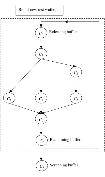
measuring the quality of an etching process is used to explain these steps. The preprocessing step is to deposit a film on the wafer. The in-use step measures the thickness of the film before and after the etching process to monitor the process quality. The cleaning recycle step, as mentioned above, is to remove the film and clean the test wafer for reuse. The downgrade step is to deliver the test wafer to lower-grade buffers. The downgrade relationship among the test buffers is a directed graph (Fig. 1). The grinding reclaim step is to grind off some 20-30um silicon materials from the test wafer for reuse; a reclaimed test wafer is functionally like a brand-new one.

Much literature on test wafers has been published. Wong and Hood (1994) studied the impact on cycle time and throughput caused by increasing the number of process monitoring, which consequently increases the demand of test wafers. Wu (1997) examined the dispatching policy of test wafers and product wafers in the preprocessing stage. Popovich et al. (1997) developed an automated ordering process to maximize the reuse of test wafers. Chu (1998) investigated the policy for setting safety stock level in each test wafer buffer. Watanabe et al. (1999) proposed a procedure to increase the use ratio of reclaimed test wafers. Some other addresses the downgrade decision problem; that is, how many test wafers should be delivered to each of its descendant buffers from a particular buffer. Some studies (e.g., Foster et a., 1998; Chen and Lee 2000; Chen 2003) developed the downgrade decision methods by considering the instantaneous WIP level and demand of test wafers. Lu (2003) analyzed the cost structure of test wafers and solved the problem by considering the long-term demand and supply of each buffer. In summary, most previous studies focused on the improvement of operation policies for test wafers, under a given set of system parameters. Yet, very few examine the improvement of these system parameters, such as yield rates of recycle processes, for reducing the use of test wafers.

recycle processes. The decision problem is to determine the target yield rate of each buffer so that the use of brand-new test wafers can be minimized under a given budget for yield improvement. We adopt the downgrade decision model developed by Lu (2003) to determine the usage of brand-new wafers for a particular set of recycling yield rates. Changing the set of yield rates will change the usage of brand-new test wafers. Two solution methods are developed to find a set of yield rates in order to minimize the usage of brand-new test wafers. These two solution methods involve a genetic algorithm (GA) and a marginal allocation algorithm.

The remainder of this paper is organized as follows. Section 2 reviews the downgrade decision model developed by Lu (2003). Section 3 describes the problem of planning the yield improvement of cleaning recycle. Section 4 presents the two solution methods as well as the experiment results. Experiment results are presented in Section 5 and concluding remarks in Section 6.

2. Downgrade Decision Model 2.1 Cost Analysis

The cost of test wafers in a fab involves three major items: (1) the cost of machine idleness due to lack of test wafers, (2) the usage cost of test wafers, and (3) the storage cost of test wafer (WIP) in shop floor. By interviewing several 8” fab sites in industry, Lu (2003) estimates that the storage cost of test wafers is about 2.4% of the usage cost; and is at most 5% of the machine idleness cost.

From the cost analysis, the safety stock level of test wafers can be assumed to be high enough to always fulfill the time varying demand. Based on such an assumption, Lu (2003) modeled the downgrade decision as a static decision problem. That is, the input and output average daily flow rates of each test wafer buffer should be balanced.

2.2. Downgrade Decision Problem

In a typical fab, the downgrade relationship among test wafer buffers is a directed graph. Referring to Fig.1, the directed graph involves four types of buffers. Working buffers (c1-c6)

directly supply test wafers to tools. The releasing buffer (c0) releases brand-new or reclaimed

test wafers to working buffers. The reclaiming buffer (c7) reclaims test wafers, and sent them

to either the releasing buffer or the scrapping buffer. The scrapping buffer (c8) scraps the test

wafers that cannot be reclaimed further.

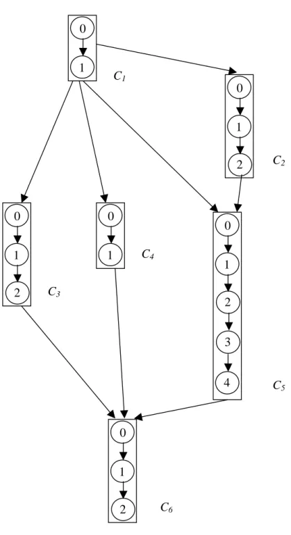
A working buffer stores m categories of test wafers, where m denotes the maximum number of cleaning recycles. Category i (1≤i≤m) represents test wafers that have received

i times of cleaning recycle. A test wafer in category i, after receiving one more cleaning

recycle, becomes one in category i+1. Any test wafer in a particular working buffer, whatever category it belongs to, is regarded as the same in specification. Each cleaning recycle in a

certain buffer has a distinct yield rate. Fig. 2 shows various categories of test wafers in a working buffer.

The downgrade decision problem is to determine the daily flow rate of test wafers to be downgraded among buffers in order to minimize the usage of brand-new test wafers.

2.3 Notations

Let the downgrade path between the reclaiming buffer and the releasing buffer be called the feedback path. By eliminating the feedback path, the directed graph becomes one without loop, which can be denoted by G = (V, E) where V={c0, c1,…, cr, cr+1} is a finite set of buffers

and E is a set of arcs. An arc represents an ordered pair of two buffers. A path from ci to cj

exists if one can traverse from ci to cj through passing k arcs (k≥1). If there is a path from ci

to cj, then ci is said to be an ancestor of cj, and cj is said to be a descendant of ci. Additionally

including the feedback path, the overall downgrade relationships can be denoted by S = (G, f), where f is the arc cr→c0. Referring to S= (G, f), the following notations are used to formulate

the downgrade decision problem.

Designations and Sets

ci: designation of test buffer i; 0≦i≦r+1, c0 is the releasing buffer; cr is the reclaiming buffer, cr+1 is the scrapping buffer, and ci (1≦i≦r-1) is a working buffer.

P(i): the set of ancestor buffers of ci in diagraph G, excluding c0; i.e. c0 ∉P(i) S(i): the set of descendant buffers for ci in diagraph G

Parameters

Di: average daily demand of test wafers in ci, 1≦i≦r-1 m(i): maximum number of cleaning recycle in ci, 1≦i≦r-1

] [k

i

r : the yield of k-th cleaning recycle in ci, 1≦k≦m(i) n: maximum number of grinding reclaim in cr

] [k

h : the yield of k-th grinding reclaim in cr, 1≦k≦n Variables

Oij: daily quantity of test wafers downgraded from ci to cj in diagraph G

Ni: daily quantity of brand-new test wafers downgraded to ci from c0, 1≦i≦r-1 N: daily quantity of brand-new test wafers downgraded from c0;

∑

− = = 1 1 r i i N N

Yi: daily quantity of reclaimed test wafers downgraded to ci from c0 ]

[k

Z : daily quantity of test wafers, with k times of reclaim, sent to c0 from cr Z: daily quantity of reclaimed test wafers sent to c0 from cr,

∑

= = n k k Z Z 1 ] [ ] [k

2.4 Model

Lu (2003) formulates an LP model for the downgrading decision as follows. The model assumes that the input flow rate should equal the output flow rate for each buffer. Otherwise, the WIP level of each buffer may increase to infinity.

Min

∑

− = 1 1 r i i N s. t.

∑

∑

− = − = + = + 1 1 1 1 r j j r j j Y N Z N (1) Nj + Yj +

∑

∈P( j) i Oij = ] 0 [ j X 1≤ j≤r−1 (2) ] 1 [ ] [ ] [ ₋ ⋅ = k j k j k j r X X 1≤ j≤r−1 (3)

∑

= ) ( 0 ] [ j m k k j X = Dj 1≤ j≤r−1 (4)

∑

∈s( i) j ij

O

= X0[0] 1≤ j≤r−1 (5) =

∑

∈P( r) j jr O _{, 1} 1 ] [ + = +

∑

rr n k k O Z 1≤ j≤r−1 (6) N h Z[1] = [1]⋅ (7) ] 1 [ ] [ ] [k ₌ k _⋅ k− Z h Z (8) N Or,r+1 = (9) 0 ; 0 ; 0 ; 0 ≥ ≥ ≥ ≥ i i ij i Z Y O N (10)

The objective function is to minimize the daily usage of brand-new test wafers. Constraint (1) denotes the flow balance relationship in buffer c0. Constraints (2) indicate the

inputs to a working buffer. Constraints (3) describe the yield relationship of a cleaning recycle in a working buffer. Constraints (4) denote that the demand in a working buffer ci is supplied

by several categories of test wafers. Constraints (5) indicate the output of a working buffer. The left-hand side describes where the output test wafers are downgraded. The right-hand side denotes the sources of the output.

Constraint (6) denotes the flow balance relationship of the reclaiming buffer cr. The

inputs are from all working buffers, represented in the left-hand side. The output involves two types of reclaimed test wafers, either within specification for reuse or out-of-specification for scrapping. Constraints (7) and (8) represent the yield relationships of grinding reclaim. Constraint (9) denotes that flow balance of the whole fab; that is, all the brand-new buffers

finally have to go to the scrapping buffer cr+1. Constraints (10) denote that all variables are

non-negative.

3. Problem of Planning Yield Targets

The decision problem of planning the recycle yield rate for each working buffer is discussed below. The cleaning recycle of test wafers is usually executed in a wet etch process. That is, putting test wafers in chemical solution for some time to clean the surface of test wafers. By changing recipes and process parameters, such as solution concentration or the time of bathing, the yield rate of recycle would change. Engineers need to experiment for the yield improvement. According to engineers’ experiences, the higher is the target yield improvement, the more is the number of experiments and consequently the higher is the cost incurred.

To explain the yield planning problem, the following notations as well as those presented in Section 2 are referred.

Notations

R = [R1, R2, …, Rr-1]: the current yield vector of the fab, where Ri = [ri[1],ri[2],...,ri[m(i)]]:

denotes the current yields at buffer ci and ri[k]is the yield of k-th recycle.

] ~ ,..., ~ , ~ [ ~ 1 2 1 ₋ = R R Rr

R : a new yield vector of the fab, where Ri

~

= [r~i[1],r~i[2],...,~ri[m(i)]] denotes the

new yields at buffer ci and ~ri[k]is the new yield of k-th recycle.

X = [X1, X2, …, Xr-1]: an yield improvement plan, where Xi = Ri

~

– Ri =

[ x_i[1],x[_i2],...,x[_im(i)] ]denotes the yield improvement targets at buffer ci, and

] [ ] [ ] [ ~ k i k i k i r r

x = − denotes the yield improvement target of k-th recycle

C(x_i[k]): the cost incurred for the yield improvement in k-th recycle at buffer ci

C(X) = ( [ ]) 1 1 ) ( 1 k i r i i m l x C

∑∑

− = =

: the cost incurred for a yield improvement plan X

B : the budget for improving the recycle yield of working buffers

The LP model presented in Section 2 can be alternatively interpreted as N = L (R). That is, given a yield vector R, the LP model L can compute the minimum daily usage of brand-new test wafers N. The problem of planning yield improvement targets can thus be formulated as follows.

Max L(R)–L ( R~) X = R~–R

B X C( )≤

The decision variables are represented by a yield improvement plan X. The objective function is to maximize the saving in the usage of brand-new test wafers, under a given budge

B.

4. Solution Methods

Two solution methods have been developed for solving the yield planning problem. One is a genetic algorithm and the other is a marginal allocation algorithm.

4.1 Genetic Algorithm

Genetic algorithm (GA) techniques, widely applied in various areas, are a random-search method for locating efficiently a near-optimal solution in the enormous space (Holland 1975; Gen and Chen 2000; Chen et al. 2001). A GA is an iterative procedure that maintains a constant-sized population P(t) of candidate solutions (called chromosomes). During each iteration step t, called a generation, new chromosomes are created by invoking some genetic

operators. Each existing and newly generated chromosome is evaluated to determine its fitness value, which denotes how good the solution is. Based on these evaluations, a set of

chromosomes are chosen by a selection procedure to form the new population P(t+1). The procedure is iteratively performed until the termination conditions are met.

The proposed GA for solving the yield planning problem is presented below.

A. Chromosome and Initial Population

A chromosome, a yield improvement plan, is denoted by X = [X1, X2, .., Xr-1] consisting

of r-1 strings, where a string Xi = [xi[1],x[i2],...,xi[m(i)]] contains m(i) positive numbers. Let

UB(x[k_i ]) represents the upper bound of x[k_i ] and the interval [0, UB(x[k_i ])] be divided into n

segments, where n = round-up(

d x UB( _i[k])

). Each of the first n-1 segments has a distance d, and the distance of the last segment is UB(x[k_i ])-(n-1)d. The value of x[k_i ] is chosen from the set

of the n+1 end points, denoted by S(x_i[k]). Let N be the total number of chromosomes in _p

chromosomes.

B. Fitness Function

The fitness function of X is defined as follows, where the first term denotes the objective function.

F(X) = [f(R) – f( R~)] – Y [C(X) – B],

where Y = 0 if C(X)≤B

= M else, where M is a very large positive number

The second term is a penalty function (Rietman and Frye 1996), which leads to a small fitness value if the solution violates the budget constraint. A chromosome with a small fitness value is less likely to survive during the evolution of the population and tends to finally be excluded from the population. The penalty design is to keep “good genes” in the population. For a budget violation chromosome, particular segments of its genes may exactly match a part of the optimum solution. Possibly carrying good genes, violation chromosomes shall not be forcibly excluded from each population.

C. Crossover and Mutation Operators

The proposed GA defines two genetic operators, crossover and mutation, to create new chromosomes.

The crossover operator is designed to create N_p×P_cr new chromosomes in each generation, where P is a predefined crossover probability. This operator is applied by first cr

randomly choosing Np×Pcr chromosomes from P(t) and randomly grouping them into

2 / )

(N_p×P_cr pairs. For each pair of chromosomes, a position in a chromosome (called the

crossover point) is randomly chosen, and the segments to the right of the crossover point

exchanged.

The mutation operator is designed to create Np×Pmu new chromosomes from P(t),

where P is a predefined probability of mutation. This operator is applied by first randomly mu

selecting N_p ×P_mu chromosomes from P(t). For each chosen chromosome, a gene x[k_i ] is randomly selected and is subsequently replaced by a number randomly chosen from the set

D. Selection Strategy

The chromosomes in population P(t) and the newly created chromosomes are put in a

pool, called S, where the number of chromosomes is h=Np ⋅(1+Pcr +Pmu) . N p

chromosomes are to be selected from S to the population P(t+1), by the rank-space method (Winston 1992) for preventing the genetic search from becoming trapped at a local optimum solution. The procedure of the rank-space method is presented below.

Step 1: Sort in descending order the chromosomes in S according to their fitness values. Let

h

Z Z

Z1, 2 ,..., be the sorted result. Such a ranking of Z , termed quality-ranking, is i

represented by Rq(Zi).

Step 2: Move the best quality-ranking chromosome from S to P(t+1). }; {Z₁ S S = − 1 ) 1 (t Z P + ← ; 1 1 Z

Y = ; /* rename the chromosome selected for P(t+1) */

N = 1 ; /* count the chromosome number in P(t+1)*/

Step 3: For each chromosome Z in S, compute the diversity index i D(Zi)

∑

= − = N k i k i Y Z Z D 1 1 ) ( ; /*Yk is a chromosome in P(t+1) */

Step 4: Sort in ascending order the chromosomes in S according to D(Zi). Such a ranking of

i

Z , termed diversity-ranking, is represented by Rd(Zi).

Step 5: Compute the sum of quality-ranking and diversity-ranking of Z in S i

) ( ) ( ) (Zi Rq Zi Rd Zi T = +

Step 6: Sort in ascending order the chromosomes in S according to T(Zi). Such a ranking of

i

Z , termed combined-ranking, is represented by Rc(Zi).

Step 7: For each chromosome in S, compute the probability of putting Z in i P(t+1)

) ( i c Z

R

r= ;

Prob(Z_i)= p⋅(1− p)r−1; /* p is a predefined probability, typically set to 0.667*/

Step 8: Generate a random number and determine which chromosome in S is selected. Let Z m

be the selected chromosome.

};S =S−{Zm /*Move Z from S to m P(t+1)*/ m Z t P( +1)← ; m m Z

Y = ; /* rename the chromosome selected for P(t+1) */ 1

+ = N

N ; /* update the chromosome number in P(t+1) */ Step 9: Termination Check

If N < Np then go to Step 3

Else Stop

E. Terminating Conditions

Population )P(t is iteratively updated until a particular chromosome keeps the best solution for over NG generations or NE generation has been created.

4.2 Marginal Allocation Algorithm

The proposed marginal allocation algorithm is an analytical method. The idea of this algorithm is by computing the cost and benefit caused by one unit yield improvement for each recycle at each buffer. Then, select the one, which is the most beneficial and meets the budget constraint, to update the yield parameters. The process is repeated until the cost incurred is over the budget. The procedure of this algorithm is presented below.

Step 0: Initialization and Function Definition

X = [0, 0, …,0]; i.e., x_i[k]= 0, for 1≤i≤r−1;1≤k≤m(i)

k i

E : a unit vector by replacing the value of x[k_i ] in X by 1

k = Up_Arg(Rik

~

) /*define function Up_Arg()*/

i = Low_Arg(Rik

~

) / *define function Low_Arg()*/

Step 1: Compute the benefit of increasing yield by one unit of d

X R Rik ( ~ + = +d⋅Eik); for 1≤i≤r−1;1≤k ≤m(i)

Step 2: Select the most beneficial alternative )) ~ ( ( _ , k i k i R Arg Up p=

_Max

; for 1≤i≤r−1; 1≤k ≤m(i) )) ~ ( ( _ , k i k i R Arg Low q=

_Max

; for 1≤i≤r−1; 1≤k ≤m(i) Step 4: Check if the cost is within the budget

If C(X +d⋅E_qp) > B then return X; Stop

Go to Step 1

5. Experiment Results

Experiments for justifying the two solution methods are executed by using a simplified fab involving six working buffers as shown in Fig. 1. The daily demand of test wafers and the current yield rate of each recycle at each working buffer are listed in Table 1. Assume

) (x[k_i ]

UB = 9% for 1≤i≤r−1and1≤k ≤m(i). The cost function for improving the yield of

k-th recycle at each buffer is the same, i.e., C(x[k_i ])= C(x[k_j]) for i≠ , as shown in Table 2. j

The budget for yield improvement is B = $50,000 and the unit yield increment is d = 1%. The current daily usage rate of brand-new test wafers, computed by the LP model, is L(R) = 1188.79. Table 3 shows the cost and benefit of the solution obtained by applying the marginal allocation method, where L(R~)=1036.76. Notice that buffers c1, c2, and c6 are not suggested

to improve the yield at the present budget. This implies that their local improvements have very few or no impact to the global improvement. Buffer c5 has the highest priority for yield

improving. Such a yield target planning can effectively guide engineers to prioritize their jobs in order to maximize their contributions.

The GA is coded in C++ which calls the downgrade decision LP model implemented in CPLEX. The parameters of GA are set as follows: Pcr = 0.8, Pmu = 0.05, Np = 100, NG = 500,

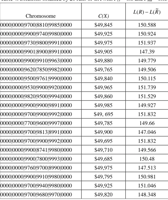
and NE = 10,000. Table 4 shows the results of 20 experiment runs. These 20 different yield

improvement plans are quite close in the C(X) and L(R)−L(R~). The mean of L(R)−L(R~) is 150.09 and the standard deviation is 1.526.

The results obtained by the marginal allocation method are slightly better than those obtained by GA. Also, the computation time per run for GA takes about 30 min. while that for the marginal allocation method takes only 10 sec. A typical fab may include more than 100 working buffers, which implies that a chromosome may involve 400 genes. Accordingly, the computation time of GA method may increase substantially. The marginal allocation method seems better in solving the addressed problem in the real world.

6. Concluding Remarks

This research formulates and solves a problem for planning the yield targets of test wafer recycle processes. Test wafers are used for monitoring tool or process quality in semiconductor manufacturing. Test wafers after use are often recycled for possible reuse. A test wafer allows a limited number of recycles. The cost and benefit for improving the yield rate in each recycle at each buffer may be different. The addressed problem is to determine the

allocation of yield improvement targets in order to maximize the benefit under a given budget. An LP model is used to evaluate the benefit of a yield improvement plan, by computing the minimum daily usage of brand-new test wafers. Based on the benefit evaluation module, two methods for finding an optimum yield improvement plan are proposed. One is the genetic algorithm and the other is the marginal allocation algorithm. The solution obtained by the marginal allocation method is slightly better, which also takes much less time in computation. This fast computation feature becomes much more important when the problem size substantially increases.

The solution of the addressed problem can effectively guide engineers to prioritize the jobs of yield improving in order to maximize their contributions. Inappropriate priority setting may increase the yield of a particular buffer but have very little or no impact to the saving of brand-new test wafers.

Acknowledgement

The authors would like to thank TSMC (Taiwan Semiconductor Manufacturing Corp.) in characterizing this research problem.

References

Chen HC (2003) Control and dummy wafers management. PhD Dissertation, National Chiao Tung University, Hsin-Chu, Taiwan

Chen JH, Fu LC, Lin MH, and Hunang AC (2001) Petri-net and GA-based approach to modeling, scheduling, and performance evaluation for wafer fabrication. IEEE Transactions on Robotics and Automation, 17(5): 619-636

Chen HC, Lee CE (2000) Downgrading management for control and dummy wafers. Journal of the Chinese Institute of Industrial Engineers, 17:437-449

Chu YF (1998) The inventory management model for control and dummy wafers. Master Thesis. National Chiao Tung University, Hsin-Chu, Taiwan

Gen M, Cheng R (2000) Genetic Algorithms and Engineering Optimization. John Wiley & Sons, New York

Foster B, Meyersdorf D, Padillo JM, and Brenner R (1998) Simulation of test wafer consumption in a semiconductor facility. IEEE/SEMI Advanced Semiconductor Manufacturing Conference, pp. 298-302

Holland JH (1975) Adaptation in Neural and Artificial Systems. Ann Arbor, MI: Univ. Michigan Press.

Lu KS (2003) Decisions for downgrading control/dummy wafers in semiconductor fabs. MS Thesis, National Chiao Tung University, Hsin-Chu, Taiwan

Popovich SB, Chilton SR, and Kilgore B, (1997) Implementation of a test wafer inventory tracking system to increase efficiency in monitor wafer usage. IEEE/SEMI Advanced

Semiconductor Manufacturing Conference, pp.440-443

Rietman EA and Frye RC (1996) A genetic algorithm for low variance control in semiconductor device manufacturing: some early results. IEEE Transactions on Semiconductor Manufacturing, 9:223-229

Watanabe A, Kobayashi T, Egi T, and Yoshida T (1999) Continuous and independent monitor wafer reduction in DRAM fab. IEEE International Symposium on Semiconductor Manufacturing Conference, pp.303-306

Winston PH (1992) Artificial Intelligence. Addison-Wesley USA, pp. 520-527

Wong CY, Hood SJ (1994) Impact of process monitoring in semiconductor manufacturing. IEEE/CPMT International Electronics Manufacturing Technology Symposium, pp.221-225

Wu JE (1997) The construction of dispatching rule for control wafer in diffusion area. Master Thesis, National Chiao Tung University, Hsin-Chu, Taiwan

Table 1: Daily demand and current recycle yields at working buffer cj

Table 2: Cost function of yield improvement for k-th recycle at each buffer Table 3: Solution obtained by marginal allocation method

Table 4: Solutions obtained by 20 runs of GA

Figure 1: Downgrade relationships among test buffers

Table 1: Daily demand and current recycle yields at working buffer cj c1 c2 c3 c4 c5 c6 Dj 3665 2538 2226 2336 6110 1448 ] 1 [ i r 90% 90% 90% 90% 90% 90% ] 2 [ i r 80% 80% 80% 80%- 80% 80% ] 3 [ i r 70% 70% 70% 70% 70% 70% ] 4 [ i r 60% 60% 60% 60% 60% 60%

Table 2: Cost function of yield improvement for k-th recycle Variable

definition Cost Function

y =x _i[1]

C

(

y

)

=

100

+

450

y

+

30

y

2 y =xi[2] 2

35

500

100

)

(

y

y

y

C

=

+

+

y =xi[3] 2

40

550

100

)

(

y

y

y

C

=

+

+

y =x_i[4] 2

45

600

100

)

(

y

y

y

C

=

+

+

Table 3: Cost and benefit of the solution obtained by marginal allocation method Chromosome C(X) L(R)−L(R~) 0000|0000|9800|9900|9991|0000 $49,985 152.03

Table 4: Solutions obtained by 20 runs of GA with Pcr = 0.8 and Pmu = 0.05 Chromosome C(X) ) ~ ( ) (R L R L − 0000|0000|9700|8810|9985|0000 $49,845 150.588 0000|0000|9900|9740|9980|0000 $49,925 150.924 0000|0000|9730|9800|9991|0000 $49,975 151.937 0000|0000|9901|8900|8991|0000 $49,905 147.39 0000|0000|9900|9910|9963|0000 $49,880 149.779 0000|0000|9620|7850|9982|0000 $49,765 149.506 0000|0000|9500|9761|9990|0000 $49,840 150.115 0000|0000|9530|9900|9920|0000 $49,965 151.739 0000|0000|9820|9500|9994|0000 $49,860 151.529 0000|0000|9900|9900|9891|0000 $49,985 149.927 0000|0000|9700|9900|9992|0000 $49, 695 151.832 0000|0000|7700|9600|9997|0000 $49,785 149.66 0000|0000|9700|9813|8991|0000 $49,900 147.046 0000|0000|9700|9900|9992|0000 $49,695 151.832 0000|0000|9900|8741|9980|0000 $49,710 149.566 0000|0000|9900|7800|9993|0000 $49,685 150.48 0000|0000|9760|9700|8990|0000 $49,975 147.513 0000|0000|9900|9910|9980|0000 $49,795 150.981 0000|0000|9700|9940|9980|0000 $49,925 151.046 0000|0000|9700|9680|9970|0000 $49,820 148.348

Figure 1: Downgrade relationships among test buffers C1 C2 C3 C4 C5 C6 Releasing buffer Reclaiming buffer Brand-new test wafers

C7

Scrapping buffer

C0

Figure 2: A working buffer stores several categories of test wafers 1 2 0 1 0 1 2 0 1 0 C1 C2 C3 C4 C5 1 2 0 3 4 1 2 0 C6

計畫成果自評

(1) 究內容與原計畫相符程度：相符

(2) 達成預期目標情況：良好

(3) 研究成果之學術或應用價值：已經接受兩篇SCI的國際期刊

M. C. Wu, C. S. Chien, and K. S. Lu, “Downgrade decision for control/dummy wafers in a fab,” International Journal of Advanced Manufacturing Technology,

SCI

M. C. Wu, C. S. Chien, and K. S. Lu, “Downgrade decision for control/dummy wafers in a fab,” International Journal of Advanced Manufacturing Technology,

參加國際會議心得

本人於2005年7月28日到7月30日參加由ACME 學會所舉辦的2005 亞太地區管理 學術研討會(International Conference of Pacific Rim Management)。此會議已經舉辦15屆，

本屆（第15屆）會議在美國聖地牙哥舉行。會議重點以亞太地區管理相關議題為主軸，

與會學者大都是華人，來自美國、加拿大、台灣、香港、新加坡、中國大陸等地。

本人覺得這個會議最大的優點是可以將所有華人的學者群聚一堂，可以快速瞭解和溝

通， 以瞭解研究發展的趨勢，並且建立未來與國外大學合作的管道。

附件：參加 2005ACME Conferenec 所發表之論文

SEMICONDUCTOR DISPATCHING BASED ON LINE-BALANCING AND LOT-ATTRIBUTES

Muh-Cherng Wu and Ting Uao Hung

Department of Industrial Engineering and Management National Chiao Tung University

Hsin-Chu, Taiwan (ROC) Tel: 886-35-731913

Abstract: This paper presents a dispatching algorithm for a semiconductor fab which has a feature called machine-dedication, a constraint imposed on the process route. The performance criterion is hit rate, the percentage of on-time completion. Simulation experiments show that the proposed algorithm outperforms previous major methods for short-routing process, and very close to the best for long-routing processes.

INTRODUCTION

Semiconductor manufacturing is more complicated than most other production processes, due to with re-entry process routes and unexpected machine failures. Reentry process routes denote that a wafer lot has to enter a tool group several times; and in each enter an operation is to be processed. Herein, a tool group is one that involves several functionally identical machines. The product completion time of a semiconductor fab is thus complex and unpredictable, consequently leading to low hit rate—the percentage of on-time completion. This paper addresses how to use dispatching to improve the hit rate of a make-to-order

semiconductor fab.

Dispatching is to determine which wafer lot to process first, while a number of lots are waiting before an available machine. Much research on semiconductor dispatching has been published, a few representative ones include Wein (1988), Lu, Ramaswamy andKumar (1994), Kim, Kim, Lim and Jun (1998), Dabbas and Fowler (2003). Yet, the fab concerned by most of these studies did not address a phenomenon known as machine-dedication, a constraint imposed on the process route due to the advance of manufacturing technology.. As stated, a wafer lot has several operations to be processed by a tool group. For a non-dedicated tool group, any machine in the tool group can freely process the associated operations of a lot. Yet, for a dedicated tool group, the associated operations of a lot have to be all dedicated to a particular machine.

A recent study (Wu, Huang, Chang, and Yang 2004) emphasized the machine-dedication feature, and proposed an algorithm (called LBSA) for a semiconductor fab to improve the hit rate. The LBSA dispatching algorithm outperforms many other algorithms for short-routing products, but not so for long-routing products. This paper presents a method that enhances the LBSA algorithm in order to achieve good performance in both short-routing and long-routing products.

DISPATCHING ALGORITHMS

In a fab, machines can be classified into two types: series and batch. A series machine processes a wafer at a time until a lot of wafers are completed, while a batch machine processes several lots of wafers at a time. This research focuses on the dispatching of series machines.

Dispatching for Dedicated Machines

The dispatching for dedicated machine is developed based on two paradigms: (1) keeping the production line balance and (2) giving higher priority to the lots that tend to be urgently late.

The line-balance paradigm models a production route by a number of segments. Each segment is ended with an operation processed by a dedicated-machine. A dedicated machine, with relatively higher investment cost, is usually the bottleneck of throughput. Due to the reentry characteristics, a dedicated machine has to process the WIPs located in many segments. Appropriately dispatching these WIPs could therefore control the throughput of each segment. The idea of the line-balance paradigm is keeping the throughput of each segment as uniform as possible. Higher throughput on a particular segment tends to produce its WIPs earlier than expected; and lower throughput tends to delay the WIP progress. Consequently, non-uniform throughput would reduce the resulting hit rate. Therefore, we give highest dispatching priority to the segment that has the highest throughput. If more than one lots are in the segments, CR (critical ratio) is used to prioritize the dispatching of lots. Here, CR, a

popular index in dispatching, refers to the ratio of the remaining time divided by the remaining processing time of a lot.

Such a line-balanced approach may have a drawback. Lots that are substantially delayed but located in a low-priority segment have little chance to remedy their progresses. To overcome the drawback, we define an exception to the application of the line-balance approach. The exception is that lots urgently late in progress, irrespective of which segments they might stay, always have higher dispatching priority than all other lots and CR is used to prioritize them.

Detail steps of the dispatching algorithm for dedicated machines are presented below, with its notation firstly explained. Consider a fab that produces only one product family that has a product route with s segments. Let Lij denote the j-th lot in segment i. The processing

time of Lij is represented by tij, and its CR value is by CR . The average cycle time of ij

segment i is represented by CTi and the number of lots in segment i is represented by n(i).

Step 1：Check if urgently late lots exist

Delay_Set = {Lij |CR_ij ≤γ，1≤i≤s;1≤ j≤n(i)} Step 2：Dispatch If Delay_Set≠ , Then φ (* , *) ( ) ij CR ArgMin j

i = for all Lij∈Delay_Set

Elseif Delay_Set = φ ，

Compute average flow rate of segment i ,

i i n j ij i t /CT ) ( 1

∑

= = ν ; 1≤i≤s Identify highest priority segment i*=ArgMax(νi); for 1≤i≤s

Prioritize highest priority lot, ( *)

* j i CR ArgMin j =

Step 3: Output the lot to be dispatched L_i*_j*; STOP.

Dispatching for Non-dedicated Machine

A starvation avoidance paradigm is proposed for the dispatching of non-dedicated machine. As stated, the ending operation of a segment is processed by a dedicated machine, which is bottleneck and critical to the fab throughput. Therefore, non-dedicated machine should be so dispatched that dedicated machines would not be starving.

Detail steps of the dispatching algorithm for non-dedicated machines are illustrated below, based on the following notation. Consider a fab with K dedicated machines, of which a non-dedicated machine is to be dispatched. The WIPs in segment i has K types; each type is

assigned to a particular dedicated machine. Let the total number of WIPs in segement i be represented by

_∑

= K k k i n 1 ) ,

( , and Lijk represent the lot associated with dedicated machine k, located

in segment i, and 1≤ j≤n(i,k)is the lot identification. Step 1：Check if urgently delay lots exist

Delay_Set = {Lijk | CR_ijk ≤γ , 1≤i≤s;1≤ j≤n(i,k)}

Step 2：Dispatching If Delay_Set≠φ ，then (* , *, *) ( ) ijk CR ArgMin k j

i = for all Lijk∈Delay_Set

Elseif Delay_Set = φ ， Compute i k i n j ijk ik CT t

∑

= = ) , ( 1 ν ; 1≤i≤s , 1≤k≤K ) ( ) , (* * ik ArgMax k i = ν for 1≤i≤s, 1≤k≤K * _{( * *)} jk i CR ArgMin j =

Step 3: Output L_i*_j*_k*, the lot to be dispatched; STOP

PERFORMANCE COMPARISON

By simulation, the proposed dispatching algorithm in terms of the hit rate performance has been compared with the LBSA and CR algorithms. The scenario of the simulation was provided by a fab in the real world. Three logistic product families, which involve 1P3M, 1P5M and 1P7M (M means metal layer), are used in the comparison. The higher the number of metal layers the longer the process route.

Experiment results show that the proposed algorithm outperforms the LBSA algorithm in all three tested products; much better than CR in short-routing products (1P3M and 1P5M), and is slightly worse than CR in long-routing products such as 1P7M. Statistic testing indicates that the difference is not significant.

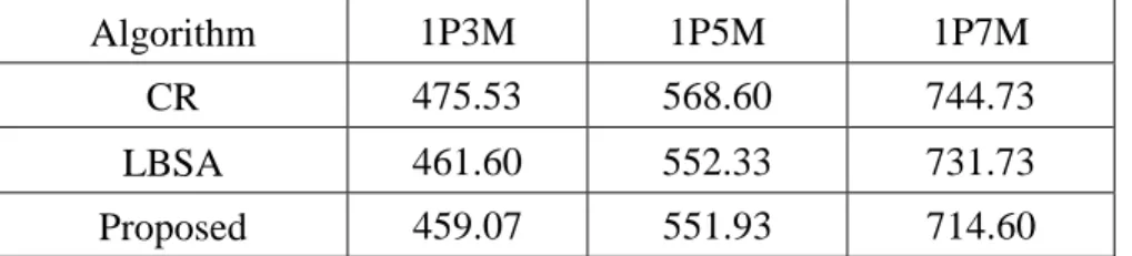
In terms of some other performance measures such as mean cycle time, the proposed algorithm also performs well, better than the other two in all tested products (Table 2).

Algorithm 1P3M 1P5M 1P7M

CR 66.99 % 75.55 % 96.67 %

LBSA 87.22 % 88.94 % 70.80 %

Table 1: Comparison of hit rate

Algorithm 1P3M 1P5M 1P7M

CR 475.53 568.60 744.73

LBSA 461.60 552.33 731.73

Proposed 459.07 551.93 714.60

Table 2: Comparison of mean cycle time

CONCLUDING REMARKS

This paper presents a dispatching algorithm for semiconductor manufacturing with machine-dedication feature. The feature is a constraint imposed on the process route, which has just recently appeared due to the advance of manufacturing technology and did not get too much attention in previous relevant literature. A recently developed algorithm LBSA, which addresses the feature, has shown good performance in hit rate for short-routing products but not well for long-routing products.

The proposed algorithm outperforms the LBSA algorithm both in hit rates and mean cycle time for both short and long process routes. Further comparison, including other logic products and other dispatching algorithm, is to be carried out in the near future.

REFERENCES

1. L. M. Wein, “Scheduling Semiconductor Wafer Fabrication,” IEEE Transactions on

Semiconductor Manufacturing, Vol. 1, No. 3, pp.115-130, 1988.

2. S. C. H. Lu, D. Ramaswamy and P. R. Kumar, “Efficient Scheduling Policies to Reduce Mean and Variance of Cycle-time in Semiconductor Manufacturing Plants,” IEEE

Transactions on Semiconductor Manufacturing, Vol. 7, No. 3, pp. 374-388, 1994.

3. Y. D. Kim, J. U. Kim, S. K. Lim and H. B. Jun, “Due-Date Based Scheduling and Control Policies in a Multiproduct Semiconductor Wafer Fabrication Facility,” IEEE Transactions

on Semiconductor Manufacturing, Vol. 11, No. 1, pp. 155-164, 1998.

4. R. M. Dabbas and J. W. Fowler, “A New Scheduling Approach Using Combined Dispatching Criteria in Wafer Fabs,” IEEE Transactions on Semiconductor Manufacturing, Vol. 16, No. 3, pp. 501-510, 2003.

5. M. C. Wu, Y. L. Huang, Y. C. Chang, and K. F. Yang, “Dispatching for Semiconductor Fabs with Machine-Dedication Features,” International of Advanced Manufacturing Technology (accepted for publication).