資本管制對銀行恐慌傳染現象之有效性探討 - 政大學術集成

全文

(1)國立政治大學國際經營與貿易研究所碩士論文. 政治大. 立 of Capital Requirement in The Effectiveness. ‧ 國. 學. Preventing against Bank Panic and Contagion. ‧. Phenomenon. 資本管制對銀行恐慌傳染現象之有效性探討. n. er. io. sit. y. Nat. al. Ch. engchi. i n U. v. 研究生：湯士俊指導教授：胡聯國博士. 中華民國一○○ 年六月.

(2) ABSTRACT. The financial contagion phenomenon, or the spillover effect, has become a crucial issue in recent years after the breakout of the financial crises in 2008. To deal with such problem, some regulations such as the capital requirement, has been introduced as a solution. In our paper, we develop a model based on Allen and Gale (2000) to testify whether the introduction of the capital requirement can successfully reduce the. 政治大 suffering from the regional liquidity shock. We conclude that after the introduction of 立 risks of bankruptcy and contagion phenomenon for the interbank system when. capital requirement, the bank will voluntarily hold more buffers to lower the. ‧ 國. 學. bankruptcy risk and reduce the spillover effect. What’s more, we construct an optimal. ‧. level of the capital requirement that maximize the social welfare utility and depends. sit. y. Nat. on the probability of bankruptcy, the percentage of early withdrawals, the relative cost. io. er. of capital and other parameters. By simulation, we have the optimal capital requirement at 6.375% in our benchmark case, which is a reasonable one compared. al. n. v i n with the current Basel Accord. C Finally, the paper shows h e n g c h i U that as the cost of capital is. getting lower, bank uses more capital which enhances the social welfare significantly in equilibrium, indicating the great importance of financial stability.. Keywords: Financial Contagion, Capital Requirement, Bank Buffer.. I.

(3) CONTENT ABSTRACT .................................................................................................................. I 1. INTRODUCTION.................................................................................................... 1 2. LITERATURE REVIEW ........................................................................................ 5 3. THE MODEL ......................................................................................................... 11. 3.1 LIQUIDITY PREFERENCE ..................................................................... 11 3.2 OPTIMAL RISK SHARING ......................................................................12 3.3 THE INTERBANK MARKET STRUCTURE ................................................16 4. FINANCIAL FRAGILITY ................................................................................... 18. 政治大. 4.1 LIQUIDATION VALUE AND BANK BUFFER .............................................19 4.2 BANK RUNS AND CONTAGIONS ............................................................22. 立. 5. THE SOCIAL WELFARE AND OPTIMAL CAPITAL REQUIREMENT ..... 27. ‧ 國. 學. 6. CONCLUSION ...................................................................................................... 32 7. APPENDIX ............................................................................................................. 35. ‧. al. er. io. sit. y. Nat. APPENDIX A: OPTIMAL RISK SHARING WITH CAPITAL REQUIREMENT ...........35 APPENDIX B: EFFECTIVENESS OF K TO REDUCE BANKRUPTCY PROBABILIT36 APPENDIX C: EFFECTIVENESS OF K TO REDUCE SPILLOVER EFFECT .........37 APPENDIX D: DERIVATION OF OPTIMAL CAPITAL REQUIREMENT K* ...........38. v. n. 8. REFERENCES ....................................................................................................... 41. Ch. engchi. i n U. TABLE CONTENT TABLE 1 - COMPARISON OF BASEL II AND BASEL III ............................................... 3 TABLE 2 - REGIONAL LIQUIDITY SHOCKS ................................................................ 12 TABLE 3 - REGIONAL LIQUIDITY SHOCKS REALIZATION ................................... 18 TABLE 4 - SUMMARY OF SIMULATED VALUES OF THE OPTIMAL K* ............... 31 TABLE 5 - SUMMARY OF SIMULATED BANK’S SOLVENC PROBABILITY ........ 32. II.

(4) 1. Introduction. The Global Financial Crises during 2008-2009 results in great damages to the financial system stability over the world, which raises a question about the adequacy of financial liberalization. Financial liberalization has led to financial deepening and higher growth in several countries from the history. However, it has also led to a greater incidence of financial crises, such as excess risk taking, higher. 治政大 of its property to expand the financial contagion is of the greatest emphasis because 立 the regional financial shocks to other regions and finally affect the entire system.. macroeconomics volatility, and the financial contagion. Among all these phenomena,. ‧ 國. 學. Therefore, to figure out the characteristics the contagion and develop a preventive. ‧. regulation from the policy maker’s view become the main purposes for our study. In this paper, we discuss two important issues regarding the financial contagion.. y. Nat. er. io. sit. The first one is about the financial contagion itself. What causes the contagion to happen? A commonly held view of financial crises is that they begin locally, in some. n. al. Ch. i n U. v. region, country, or institution, and subsequently “spread” out to elsewhere. This. engchi. process of the spread out is often referred to as “contagion”. What might justify contagion in a rational economy? There are two broad classes of explanations. The first class of explanations thinks that the adverse information that precipitates a crisis in one institution also implies adverse information about the other. This view emphasizes correlations in underlying value across institutions. A second type of explanation begins with the observation that financial institutions are often linked to each other through direct portfolio or balance sheet connections. For example, entrepreneurs are linked to capitalists through credit relationships; banks are known to hold interbank deposits. While such balance sheet connections may seem to be 1.

(5) desirable at the first sight, during a crisis the failure of one institution can have direct negative payoff effects upon stakeholders of institutions with which it is linked. Here we adopt the settings of Allen and Gale (2000) as our fundamental model, which is based on the assumptions of the inter-bank claims and the incomplete market structure. Because the liquidity preference shocks are imperfectly correlated across regions, banks hold interregional claims on other banks to provide insurance against liquidity preference shocks. When there is no aggregate uncertainty, the first-best allocation of risk sharing can be achieved. However, this arrangement is financially. 政治大 throughout the economy. The key here is that the possibility of contagion depends 立. fragile. A small liquidity preference shock in one region can spread by contagion. strongly on the completeness of the structure of inter-regional claims.. ‧ 國. 學. The second one is about the regulation method. According to Jean Charles. ‧. Rochet (2008), the safety and soundness regulatory instruments used in the banking. sit. y. Nat. industry could be classified into six broad types: 1. Deposit interest rate ceilings, 2.. io. er. Entry, branching, network, and merger restrictions, 3. Portfolio restrictions, 4. Deposit insurance, 5. Capital requirements, 6. Regulatory monitoring and supervision. In this. al. n. v i n paper, we emphasize on the roleCof capital requirement, h e n g c h i U which is the key focus of the Basel Accord since 19981.. The Basel Accord set a simple standard for harmonizing solvency regulations for internationally active banks of the G-10 countries. It requires that banks meet the minimum capital ratios of 4% tier 1 capital2 and 8% tier 1 plus tier 2 capital to risk-weighted assets by the end of 1992. However, it is criticized for taking too. 1. The Basel Accord, elaborated in July 1988 by the Basel Committee on Banking Supervision (BCBS), required internationally active banks from the G10 countries to hold a minimum total capital equal to 2 Tier 1 capital consists mainly of common stock and some perpetual preferred stock. Tier 2 capital includes preferred stock, subordinated debt, and allowance for loan losses. In calculating risk-weighted assets, assets are classified into 4 risk-weight categories: zero percent, 20 percent, 50 percent, and 100 percent risk-weight category. 2.

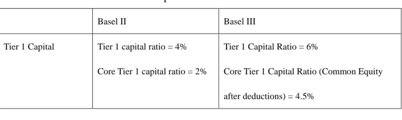
(6) simplistic an approach to setting credit risk weights and for ignoring other types of risk. After a long bargaining process of more than ten years with the banking profession, the Basel Committee on Banking Supervision announced the Basel II which relies on three pillars: minimum capital requirements for credit risk, supervisory review of an institution’s capital adequacy and internal assessment process, and effective use of market discipline as a lever to strengthen disclosure. However, since the global financial crises in 2008, the existing system of Basel II has been reviewed and questioned. Finally, at the Seoul G20 Leaders summit in. 政治大 substantial strengthening of existing capital requirements. The Committee's package 立 November 2010, the Group of Governors and Heads of Supervision announced a. of reforms increased the minimum common equity requirement from 2% to 4.5%. In. ‧ 國. 學. addition, banks will be required to hold a capital conservation buffer of 2.5% to. ‧. withstand future periods of stress, which brings the total common equity requirements. sit. y. Nat. to 7%. This reinforces the stronger definition of capital and the higher capital. io. er. requirements for trading, derivative and securitization activities to be introduced at the end of 2011. What's more, the countercyclical capital charge and forward-looking. al. n. v i n provisioning method were also C raised to deal with theU h e n g c h i procyclical risk-taking problem among the banking system. The comparison of Basel II and Basle III is showing in Table 1. TABLE 13 - Comparison of Basel II and Basel III. Tier 1 Capital. Basel II. Basel III. Tier 1 capital ratio = 4%. Tier 1 Capital Ratio = 6%. Core Tier 1 capital ratio = 2%. Core Tier 1 Capital Ratio (Common Equity after deductions) = 4.5%. 3. Resource from "Basel III: A global regulatory framework for more resilient banks and banking systems", 2010, Basel Committee on Banking Supervision. 3.

(7) The difference between the total capital requirement of 8.0% and the Tier 1 requirement can be met with Tier 2 capital. Capital Conservation. No regulation. Banks will be required to hold a capital. Buffer. conservation buffer of 2.5% to withstand future periods of stress bringing the total common equity requirements to 7%. Capital Conservation Buffer of 2.5 percent, on top of Tier 1 capital, will be met with common equity, after the application of deductions.. Countercyclical. No regulation. 立. Capital Buffer. 政治大. A countercyclical buffer within a range of 0% – 2.5% of common equity or other fully loss absorbing capital will be implemented. ‧ 國. 學. according to national circumstances.. ‧. Banks that have a capital ratio that is less than 2.5%, will face restrictions on. er. io. sit. y. Nat. payouts of dividends, share buybacks and bonuses.. al. Referred to the structure of the Basel arrangement, here we considered the. n. v i n capital requirement (k) to the C original and Gale model in order to discuss h e nAllen gchi U whether the mandatory capital regulation can effectively reduce the liquidity risk over the banking system and further prevent the bank runs from happening. In our model, the capital requirement k is the capital amount per unit of deposits the banks hold, which can be seen as the owner’s capital. The stockholders can only be rewarded in the long term, that is, we assume the stockholders have a low time preference and value the consumption at date 2. This will alter the form of the feasibility constraint. Here, the cost of capital, between. , plays an important role in our model. The relationship. and R, the return from investing in long assets, has a significant meaning. 4.

(8) over the effectiveness of the regulation. We’ll discuss the relationship in full detail in the following chapters. The rest of this paper is organized as follow. Section 2 we will review some of the related literature regarding the capital requirement, or prudent regulation. Section 3 presents the form of our model. Section 4 characterizes the equilibrium of the model when there is a minimum capital requirement. Section 5 we discuss the welfare issue, and finally in Session 6 we come to the conclusion.. 2. Literature Review. 立. 政治大. ‧ 國. 學. There are two topics in our model, the financial contagion phenomenon in the banking systems, and the government regulation of capital requirement. Regarding the first. ‧. issue, we first review the article of Allen and Gale in 19984 and 20005, with the later. y. Nat. sit. one as the main source of our model. In Allen and Gale 1998, they summarized two. n. al. er. io. traditional views of the bank panics. One is that they are “random events” and. i n U. v. unrelated to the real economy. This kind of view treats the bank panics as the result of. Ch. engchi. sell-fulfilling properties of the depositors. If everyone believes that a banking panic is about to occur, it is optimal for each individual to try to withdraw his funds simultaneously, which made the bank runs to happen. An alternative to the random view is that banking panics are a natural phenomenon of the business cycle. An economic downturn will reduce the value of bank assets, raising the possibility that banks are unable to meet their commitments and pushing the depositors to withdraw their funds. This attempt will precipitate the crisis.. 4. Allen Franklin, Gale Douglas. “Optimal Financial Crises”, Journal of Finance, 1998, vol. LIII, no. 4 Allen Franklin, Gale Douglas. “Financial Contagion”, Journal of Political Economy, 2000, vol. 108 no.1. 5. 5.

(9) Allen and Gale based on the random view and developed a model in the article in 2000 to explain how the regional bank panics to spread to other regions, which we called it as the “contagion”. In this model, they treat the misallocation and incompleteness in the financial sector and as the causes of economic fluctuations, and trying to provide some microeconomic foundations for financial contagion. The most important feature in this model is about the interbank deposit linkage among the banking system. The model assumes that there exist four different regions and the respective representative depositors and banks. Each representative bank holds. 政治大 shocks. When there is no aggregate uncertainty, the first-best allocation of risk sharing 立 interregional claims on other banks to provide insurance against liquidity preference. can be achieved. However, this arrangement is financially fragile; therefore a small. ‧ 國. 學. liquidity preference shock in one region can spread by contagion throughout the. ‧. economy. The possibility of contagion actually depends on the completeness of the. y. Nat. structure of interregional claims.. er. io. sit. Amil Dasgupta (2002) 6 established a similar model to illustrate financial contagion through the capital connection. In this article, they firstly classify two. n. al. different kinds of sources. i n ofC contagion, the adverse hengchi U. v. information among the. participators, and financial linkage within the financial institutions such as the credit relationship of the commercial banking, which is also the center of this article. They present a model of an economy with multiple banks where the probability of failure of individual banks, and of systemic crises, is uniquely determined. The cross holding of deposits motivated by imperfectly correlated regional liquidity shocks enable banks to hedge regional liquidity shocks but also lead to contagious effects conditional on the. failure of a financial institution. The conclusions of their article are that (1) there exist. 6. Amil Dasgupta, “Financial Contagion through Capital Connections: A Model of the Origin and Spread of Bank Panics”, 2004, Journal of the European Economic Association, 2(6), pages 1049-1084. 6.

(10) a specific direction of the contagion, which provides a rationale for localized financial panics; (2) there exists an optimal level of interbank deposit holdings in the presence of contagion risk, based on the probability of bank failure; (3) they demonstrate that the intensity of contagion is increasing in the size of regionally aggregate liquidity shocks.. Viral V. Acharya and Tanju Yorulmazer (2006)7 put their emphasis on the bank herding phenomenon, that is, banks choose to lend to similar industries, which maintain a high level of inter-bank correlation and erode the profit margins of the. 政治大 conclude that profit-maximizing bank owners have an incentive to herd so as to 立. banks because of the high intensity of competitions, causing the inefficiency. They. minimize the information spillover from bad news about other banks on their. ‧ 國. 學. borrowing costs and in turn on their future profits. Here, the ex ante expectation of the. ‧. poor performances by the competitive banks play as a signal of the deteriorating of. sit. y. Nat. the “common factor” that affects the economy as a whole, pushing the banks to herd. io. er. to avoid losses from higher borrowing cost if the bank failed. This paper illustrates how the information-based model works in the herding and contagion issue.. n. al. Ch. Next we turned to the second issue: the. engchi. v i n bank U capital. requirement. The. effectiveness of capital requirement has been discussed and studied for quite a long time since the introduction of the Basel Accord in 1988. The Basel Committee published an article8 to review the impact of the Basel Accord after 10 years of the initial introduction. They indicated that the main objective of the framework is to strengthen the soundness and stability of the international banking system by encouraging international banking organizations to boost their capital positions. The. 7. Viral V. Acharya and Tanju Yorulmazer, “Information Contagion and Bank Herding”, 2006, Journal of Money, Credit and Banking, 40(1), page 215-231. 8 Patricia Jackon, “Capital Requirement and the Bank Behavior: The Impact of the Basel Accord”, 1999, Bank of International Settlement, Switzerland. 7.

(11) major contribution of the article is that it summarizes several major issues of the regulation. (1) Whether the adoption of fixed minimum capital requirements led some banks to maintain higher capital ratios. (2) Do banks adjust their capital ratios to meet the requirements by increasing capital or reducing risk-weighted assets? (3) What is the impact of capital requirements on risk-taking? (4) Have banks artificially boosted their capital ratios by engaging in capital arbitrage9 and creating some side effects such as credit crunches? (5) Did the introduction of minimum capital requirements for banks harm their competitiveness and reduce competitive inequalities between banks?. 政治大 risk-weighted assets of major banks in the G-10 actually rose from 9.3% to 11.2%, 立. Regarding issue (1) and (2), the historical data in 1988-1996 showed that the. while the way the banks choose to achieve is vary according to the stage of the. ‧ 國. 學. business cycle and the bank’s own financial situation. Research suggests that banks. ‧. are likely to cut back lending to meet the capital requirements when it would be too. sit. y. Nat. costly to raise new capital. However, for issue (3) and (4), though some theoretical. io. er. papers have suggested that capital requirements applied may induce banks to substitute towards the riskier assets, engage in the arbitrage activities by. n. al. Ch. securitizations and even tighten their lending. engchi. v i n inUthe economic. downturn, no. significant empirical evidence support such views. Finally, the competitiveness and inequality issues are more difficult to study than the previous ones. The article mentioned that the response from the equity market may be a potential source, but it still needs more extensive study. Sangkyun Park (1994) 10 recognizes two main factors that cause the capital requirement to affect the weighted average cost of capital and hence the investment 9. According to C. Bajlum and P. Tind Larsen (2007), capital structure arbitrage refers to trading strategies that take advantage of the relative mispricing across different security classes traded on the same capital structure. 10 Sangkyun Park, “The Bank Capital Requirement and Information Asymmetry”, 1994, Federal Reserve Bank of St. Louis 8.

(12) behavior of banks: underpriced debt resulting from the deposit insurance and information asymmetry between managers and the stock market. For a bank enjoying a low cost of debt (deposits), an increased proportion of equity financing raises the weighted average cost of capital. When the stock market underestimates the value of a bank due to information asymmetry, equity financing is expensive. This paper finds that banks constrained by the tightened capital requirement grew slower in 1991 and that information asymmetry as well as underpriced deposits played a role in explaining the slower growth. Empirical results support that both factors contributed. 政治大 requirement, and it suggests that to mitigate the negative effect of asymmetric 立. to the slow growth of risk-weighted assets after the tightening of the capital. information by implementing the capital requirement in a flexible manner.. ‧ 國. 學. Hellmann, Murdock and Stiglitz (2000)11 specified two different effects of the. ‧. capital requirement in their article, the capital at risk effect, and the franchise value. y. Nat. effect. It is well-known that an increase in bank competition that erodes the present. er. io. sit. value of the banks’ future rents (their franchise or charter value) reduces their incentives to behave prudently. The standard regulatory response has been to tighten. al. n. v i n C himplies higher losses capital requirements: higher capital for the banks’ shareholders engchi U. in case of default, and hence lower incentives for risk-taking. However, in addition to this “capital at risk effect”, there is a ”franchise value effect” that goes in the opposite direction. Specifically, it claims that higher capital requirements reduce the banks’ franchise values, and hence the payoffs associated with prudent investment, so their overall effect is ambiguous. HMS argued that by adding the deposit rate control to the existing regulation, any Pareto-efficient outcome can be achieved since it facilitates prudent investment by increasing franchise values, and this method dominates the 11. Hellman, Murdock and Stiglitz, “Liberalization, Moral Hazard in Banking, and Prudential Regulation: Are Capital Requirements Enough?”, 2000, The American Economic Review, 90(1), page 147 - 65. 9.

(13) traditional capital requirement regulation. Few papers discuss the issue of the social welfare after the introduction of the capital requirement, and Skander J. Van den Heuvel (2007)12 is the latest one which tries to measure welfare cost of such regulation. The main contributions of this paper are to build a framework to analyze the social cost of capital requirements, to derive a simple formula for its magnitude and to use that formula to measure the welfare cost of such requirements. This paper argues that capital adequacy regulation can come with an important cost because it reduces the ability of banks to create liquidity by. 政治大 current effective capital requirement is equivalent to a permanent loss in consumption 立. accepting deposits. Based on the U.S. data and estimation, the welfare cost of the. of 0.1 to 0.2 percent (1% in another estimation), which is fairly large and beyond the. ‧ 國. 學. benefit in reducing the cost of moral hazard problems. All of these suggest that the. ‧. current capital requirements are too high. Therefore, to deal with such tradeoff. sit. y. Nat. between maintaining a relative low capital requirement and having an acceptable. io. er. probability of bank failure, to designing a more risk-sensitive system seems to be the trend in practice. However, it concludes that the stated goal of keeping capital ratios at. al. n. v i n C hbank is clearly notUjustified. about the same level for the average engchi. 12. Van den Heuvel, Skander J, 2008. "The welfare cost of bank capital requirements," Journal of Monetary Economics, Elsevier, vol. 55(2), pages 298-320 10.

(14) 3. The Model. 3.1 Liquidity Preference. At the very beginning, we describe the model where stochastic liquidity preference provides a motive for risk sharing. This framework is based on Allen and Gale (2000). There are three dates, t = 0, 1, 2, There is a single consumption good that serves as the numeraire, which can be invested in assets to produce future consumption.. 政治大 (long asset). One unit of the 立consumption good invested in the storage technology at. Two types of assets exist, including a liquid asset (short asset) and an illiquid asset. ‧ 國. 學. date t produce one unit of the consumption good at date t+1, while one unit of consumption good invested in the long asset at first date produces R>1 unites of. ‧. output at the final date. However, if the long asset is being early liquidated, each unit. sit. y. Nat. of the long asset can be prematurely liquidate to produce 0<r<1 units of the. n. al. er. io. consumption good at the middle date.. i n U. v. The economy is divided into four identical regions, A, B, C, and D. the regional. Ch. engchi. structure can be interpreted in a variety of ways, for example, a region can be correspond to a single bank, a geographical region, or a specialized sector or industry. Each region contains a continuum of ex ante identical consumers (depositors). A consumer has an endowment equal to one unit of the consumption good at date 0 and nothing at date 1 and 2. The consumer preferences are as follow, where. represents. the probability for the consumer to be an “early consumer” who value consumption only at date 1;. represents the probability for the consumer to be a “late. consumer” who value consumption only at date 2.. 11.

(15) Where. denotes consumption at date t=1, 2. The period utility function. are. assumed to be twice continuously differentiable, increasing, and strictly concave.. TABLE 2 - Regional Liquidity Shocks A. B. C. D. S1 S2. The probability. and. ,. . The realization of these random variables depends on the. 學. and. ‧ 國. possible values of. 政治大 , a high value and a low value, which is denoted by 立. varies from region to regions. We defined there are two. state of nature. There are two equally likely states S1 and S2, and the corresponding. ‧. realizations of the liquidity preference shocks are given in table 1. Note that each. sit. y. Nat. region has the same probability of having a high liquidity preference shock; the. io. er. aggregate demand for liquidity is also the same in each states. All uncertainty is. al. resolved ate date 1 when the state of nature is revealed and each consumer learns. n. v i n C h Finally, let’s U whether he is an early or late consumer. e n g c h i define the ex ante probability of being an early consumer using the average fraction. .. 3.2 Optimal risk sharing. Here we characterize optimal risk sharing as the solution to a panning problem. Since consumers are ex ante identical, we treat all consumers symmetrically. We further assume that every early consumer receives consumption c1 and very late consumer receives c2. The planner is aimed to make all the investment and consumption decisions to maximize the unweighted sum of consumers’ expected utility. 12.

(16) At the first date, the planner chooses a portfolio. subject to the. feasibility constraint at date 0. (3.1) Here x and y are the per capita amounts invested in the long and short assets, respectively. The capital requirement, k, represents the minimum required capital per unit of deposits hold by the bank to match the regulation from the authorities. Therefore, there are two different parts in the bank’s finance structure, the deposits from depositors and the owner’s capital. We can treat equation (3.1) as the accounting. 政治大 Since the total amount of consumption provided in each period is a constant, it is 立. balance as the total assets equal liabilities plus owner’s capital.. optimal to provide for consumption at date 1 by holding the short asset and to provide. ‧ 國. 學. for consumption at date 2 by holding the long asset. The feasibility constraints at date. ‧. 1 and date 2 are respectively. (3.3). er. io. sit. y. Nat. (3.2). We assume that the shareholders get the payoff of the invested capital only at. al. n. v i n C h regulations overUthe bank owners to prevent the date 2. This implies the government engchi early profit taking behaviors.. represents the cost of capital to the bank, or payoff to. the shareholder. Therefore, the return from long assets must be distributed to late consumers (depositors) and the capital owners, which shows in equation (3.3). At date 0, each consume has an equal probability of being an early or a late consumer, so the ex ante expected utility is . By adapting the logarithmic utility function ( solve the optimal allocation for. .. 13. (3.4) ) we.

(17) Subject to. The first order condition is (3.5) Thus the first-best allocation satisfies the incentive constraint (3.6) 政治大 This means the late consumers find it weakly optimal to reveal their true type 立. rather than pretend to be earl consumers. The incentive efficient allocation maximizes. ‧ 國. 學. the objective function subject to all the feasibility constraints (3.1), (3.2), and (3.3). ‧. and the incentive constraint (3.4).. n. al. er. io. sit. y. Nat. The optimal consumption and investment is as follow. (Appendix A). Ch. engchi U. v ni. (3.7) (3.8) (3.9) (3.10). Here we calculate the partial effect of. and. with respect to. . (3.11) (3.12) (3.13) (3.14). 14.

(18) Note that. is the ratio of the cost of capital to the long asset return, and it can. be seen as the measure of the “relative cost of capital” which we explained before. and. From above result, as capital requirement k goes up,. both decrease if. . This is reasonable because the injection of capital increase the resources that can be invested in the assets to support the 2-period consumption; however, if the cost of capital is too high (. , it will crowd out the long asset return that can be . As. originally distributed to. decreases, so does. because they are just different. 政治大 all certainty because the bank needs more long term asset to support the using of 立. in multiplying a long term return R. Regarding the investment side, x increases with. partial effect of increase the cost of capital. 學. is as follow, and we don’t explain more. here because of the similar logic as increasing the capital itself.. Nat. n. al. er. io. sit. y. ‧. ‧ 國. capital, thus it will allocate more to x (so less to y) if the cost of capital is high. The. Ch. engchi. i n U. v. (3.15) (3.16) (3.17) (3.18). According to Allen and Gale, the optimal sharing solution without the capital requirement is as below. We need this information to do the following comparison, so let us show the results here for reference. (3.19) (3.20) (3.21) (3.22). 15.

(19) The results are quite intuitive and straightforward. The consumers receive at date 2 if he’s a patient one.. at date 1 if he’s impatient and receive. The optimal allocation for short assets y just equals to the average probability or early withdraw,. , while the long assets x equals to. , which is perfectly matched by. the time. Note that, even if the planner cannot observe the consumers’ type, the first-best can still be achieved. By transferring resources among the. allocation. different regions, the planner can satisfy every region’s need at date 1 and date 2.. 治政 3.3 The Interbank Market Structure 大立 ‧ 國. 學. In our article, we assume an incomplete market structure from Allen and Gale (2000). ‧. which is illustrated in the figure 1. We use such structure mainly to discuss the situation for the regional bankruptcy to spread out to the whole economy. Allen and. y. Nat. io. sit. Gale have proved that, only under the incomplete market structure, the financial. n. al. er. contagion is possible for a given excess liquidity shock. They also mentioned that,. i n U. v. when there’s no overall shortage of liquidity, there is always a first-best consumption. Ch. engchi. allocation for three different market structures (complete, incomplete and disconnected) by transferring deposits among the regions. In each region there is a continuum of identical banks. We focus on a symmetric equilibrium in which all banks adopt the same behavior, and we can describe the decentralized allocation by a representative bank in each region. Without of generality, we assume that each consumer deposits his endowment of one unit of the consumption good in the representative bank in his region. The bank invests the deposits in a portfolio. and offers a deposit contract. that allows the depositor to withdraw either 16. units of consumption at date 1 or.

(20) units at date 2.. A. B. D. C. Figure 1—Incomplete Market Structure. 政治大 In the incomplete market form, the banks are allowed to exchange deposits at the 立. first date. Each region is negatively correlated with the next region (that is, bank A. ‧ 國. 學. hold deposits in Bank B, while bank D hold deposits in Bank A). This is reasonable. ‧. because in a real world the transaction and information costs may prevent banks from. sit. y. Nat. acquiring claims on banks in remote regions. We also assume that the bank holds. io. deposits in region B, and so on.. al. n. region A holds. Ch. er. deposits in the adjacent region at the first date. For example, the bank in. n U engchi. that is needed to satisfy the budget constraints.. iv. is the minimum amount. W also assume that the regions with the high liquidity shock. liquidate their. deposits in other banks at date 1 whereas banks with the low liquidity shock. do. not after the aggregate liquidity shock is observed, while the region with a high liquidity shock has deposits in a region with a low one. One characteristic of the incomplete market is that, although each region is relying on just its neighbor for liquidity, the entire economy is connected. This feature is important when discussing the financial fragility of the economy.. 17.

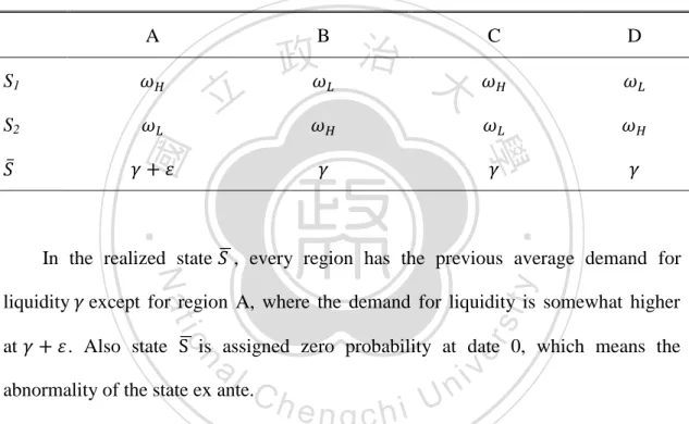
(21) 4. Financial Fragility. To illustrate the financial fragility, we fix the previous model to allow for the occurrence of a state. in which the aggregate demand for liquidity is greater than the. system’s ability to supply and show that this can lead to a global crisis.. TABLE 3 - Regional Liquidity Shocks Realization A. B. S1. 立. S2. C. 政治大. D. ‧. ‧ 國. 學. In the realized state. , every region has the previous average demand for. y. Nat. er. is assigned zero probability at date 0, which means the. al. n. . Also state. io. at. sit. liquidity except for region A, where the demand for liquidity is somewhat higher. Ch. abnormality of the state ex ante.. engchi. i n U. v. In the continuation equilibrium beginning at date 1, consumers will optimally decide whether to withdraw their deposits at date 1 or date 2. Early consumers always withdraw at date 1 while late consumers made the decisions depending on which gives them the larger consumption. On the other hand, banks are required to meet their promised to pay. units of consumption to each depositor who demands. withdrawal at date 1. If they cannot do so, they must liquidate all their assets at date 1 to support it. Once the bank meet it obligations at date 1, then the remaining assets are liquidated at date 2 and given to the late consumers. Here we note another idea of the “liquidation pecking order”. In order to fulfill 18.

(22) the demand at date 1, the banks are assumed preferable to liquidates assets in a particular order, which goes as follows: first, the bank liquidates the short asset, then it liquidates deposits in the neighboring bank, and finally it liquidates the long asset. To ensure the liquidating order, we need to following condition: (4.1) The above equation represents the cost of obtaining the liquidity by liquidating different assets. In order to maximize the interest of depositors, the bank must liquidate the assets by this order.. 政治大 At date 1 a bank can find itself 立 in one of three conditions. A bank is said to be solvent By the pecking order, we can define the terms regarding the status for the bank.. ‧ 國. 學. if it can meet the demands of every depositor who wants to withdraw by using only its liquid assets, that is, the short asset and the deposits in other regions. The bank is said. ‧. to be insolvent if it can meet the demands of its deposits but only by liquidating some. sit. y. Nat. of the long asset. Finally, the bank is said to be bankrupt if it cannot meet the. n. al. er. io. demands of its depositors by liquidating all its assets. We use these terms frequently in the following discussion.. Ch. engchi. i n U. v. 4.1 Liquidation Value and Bank Buffer. Firstly, in order to discuss the value of the deposit at date 1 if the bank is bankrupt, we need to define the “liquidation value” of the deposit,. If. , then all the. depositors will withdraw as much as they can at date 1. The mutual withdrawals will determine the value of. simultaneously and yield the same. to every depositor.. For example, bank A’s liquidation value can be shown as follow: (4.2). 19.

(23) This equation must hold for any region i where the maximum value of. . We can also calculate. and find the “upper bound” of it.. by assuming. (4.3) Now, let’s suppose that a bank is insolvent and has to liquidate some of the long asset. How much can the bank afford to give the consumers at the first date? Here comes the concept of the “buffer”, that is, the maximum amount of the long assets that can be liquidated to support the early withdrawals while keeping the late consumers satisfied at the same time (actually, the bank must give the late consumers. 政治大 and Gale defined the buffer立 as follow:. at date 2; otherwise they would be better off withdrawing at date 1). Allen. 學. ‧ 國. at least. (4.4). The logic for the buffer function is that. The bank must give the late consumers. ‧. at least. at date 2; otherwise they would be better off withdrawing at date 1. So a. y. Nat. of early consumers must keep at least. io. sit. bank with a fraction. of the. n. al. er. long asset to satisfy the late consumers at date 2. Then the amount of the long asset that can be liquidated at date 1 is. Ch. i n U. v. , and the amount of consumption. engchi. that can be obtained by liquidating the long asset without causing a run should be multiple by the early liquidating return r. We show that, by considering the capital requirement, the buffer will be larger in certain circumstances and prevent the bank runs from happening. This result comes from the comparison of the buffer in our model and that in Allen and Gale (2000). we state the result in proposition 1.. 20.

(24) Proposition 1 The bank Buffer. will be larger under the capital requirement is introduced. Proof. The original buffer of the Allen and Gale’s model is . The buffer under capital requirement in our model is . By subtracting. from. , we. can obtain the following results.. 立. 政治大. (4.5). ‧. ‧ 國. 學 er. io. sit. y. Nat. Obviously, the buffer increases after the introduction of capital requirement.. al. n. v i n C h plays an important Notice that the relative cost of capital e n g c h i U role here. Actually,. is. the sufficient condition for the bank buffer to expand. The reasons are that bases on a high cost of capital, the long assets investment increase while the consumption at state 1 decreases, leading to a larger buffer than the original one. The key here is the negative impact of the capital requirement to the early consumptions. Rafael Repullo, CEMFI and CEPR (2002) indicate an increase in the cost of capital has a negative effect on the banks’ incentives for prudent investment behavior, unless they operate in an environment with high capital requirements which has more bite for the gambling strategy. Although in our model there has no assets classified as. 21.

(25) prudent and risky, this statement can still provide some explanations for the improvement for the increase of buffer which lead to the higher banking stability.. 4.2 Bank Runs and Contagions. In this section, we discuss the conditions for the bank runs and contagions to happen, and how our model can effectively lower the possibility of these outcomes. Firstly, we reconsider the condition that the bank would be bankrupt. For example, in region A, the bank has early consumers is. units of the short asset. The fraction of. 政治大. in state , so in order to pay each early consumer. 立. units of consumption by liquidating some. 學. ‧ 國. consumption, the bank will have to get. units of. of the long asset. This is the buffer. Bank A will fall into bankruptcy if the excess is greater than the buffer plus the net value of the interbank. ‧. liquidity demands. deposits of Bank A. We show the condition in equation (4.6).. io. sit. y. Nat. (4.6). n. al. er. It’s important to talk about how the role of the interbank deposits to affect the. Ch. i n U. v. bankruptcy condition. Let’s imagine that once Bank A tries to withdraw its deposits in. engchi. other bank (Bank B), Bank B will observe such action and withdraw their deposit in Bank C as well to protect the value of their deposit. Because they think the excess liquidity demand in region A might spread to other regions and turn into a crisis, and they would like to withdraw the deposit now to get at least. rather than liquidate. the long asset (remember that the pecking order assume the bank will liquidate the deposits in other regions before liquidate the long asset). Finally, all banks will withdraw their deposit at date 1. However, the value of the deposit in Bank B is different from the deposit in Bank A, making Bank A receiving some benefits from the interbank deposits. As the 22.

(26) liquidation value. , but. because of Bank A’s liquidity. problem, bank A gets some supports from its interbank deposits to deal with the excess liquidity demand. In Allen and Gale’s article, they think the liquidation value is determined simultaneously and must be the same for all the regions. Therefore, the mutual withdrawals simply cancel out each other. We have a different opinion about this and try to apply the interbank effect into equation (4.6) to affect the bankruptcy condition. To sum up, if. is large enough and the inequality (4.6) is. satisfied, then we can infer that the bank is bankrupt. We call this inequality as the is small 政治大 enough and the inequality is not satisfied, bank A is insolvent but not bankruptcy. 立. “bankruptcy condition”. Note that, there also exist a situation when. However, the late consumers in region A are worse off because the premature. ‧ 國. 學. liquidation of the long asset at date 1 prevent the bank from paying. ‧. at date 2.. to depositors. sit. y. Nat. The second issue is about the contagion, or spillover effect, of the original. io. er. liquidity shock in region A to other regions. Once the Bank A is bankrupt, there will be a spillover effect to region D. A deposit in region D is worth. n. al. deposit in region A is worth. Ch. n U engchi. iv. and a. , so banks in region D suffer a loss when cross. holdings of deposits are liquidated. The liquidation of region D’s long assets will cause a loss to banks in region C, and this time the accumulated spillover effect large enough that region C too will be bankrupt. As we go from region to region the spillover gets larger and larger, because more regions are in bankruptcy and more losses have accumulated from liquidating the long asset. So once region D goes bankrupt, all the regions go bankrupt. Here we list the “spillover condition” . The term. is the amount promised to the banks in region C, and. (4.7) is the. upper bound on the value of deposits in region A when it is liquidated (see equation 23.

(27) (4.3)). Hence the left-hand side of the condition is the difference between liability and the upper bound on assets in the interbank deposit market for region D. If this exceeds region D’s buffer, the spillover will force banks in region D to be bankrupt. Here we show that the both of the two effects will be reduced under the introduction of capital requirement. In proposition 2 we state the result of the bankruptcy problem, and in proposition 3 we turn to the spillover effect.. Proposition 2. 政治大. Supposed the capital requirement is introduced, there will be less possibility for the. 立. bankruptcy to happen, that is,. ‧ 國. 學. We leave the complete proof in the Appendix B. From equation (4.6), we have. ‧. n. al. after and before the introduction of capital. er. io. bankruptcy in region A. By comparing. , that will trigger the. sit. Nat. equation, we can calculate the minimum liquidity shock,. . Based on. y. the bankruptcy condition. i n U. v. requirement, we can check whether the possibility of bankruptcy is getting lower.. Ch. That is, we want to testify whether where. e n g c h i the with the capital requirement,. represents the minimum liquidity shock that will trigger the bankruptcy. after the capital requirement is introduced, and. represents the one without capital. requirement. The results are as below.. (4.8) We reasonably assume that long asset. Obviously, if. for sufficient large return of the. , the denominator will be smaller and the numerator 24.

(28) will be larger, which makes the value of the ratio increase. However, we are still uncertain about the sign of the above solution. In order to figure out the net effect of the capital requirement, we take the partial derivative of. .. (4.9) This result is clear. As we raise the capital from the very beginning, the minimum level of liquidity shock. that can trigger the bankruptcy in region A becomes larger.. We conclude that, after the regulation, there is lower probability of the bankruptcy in. 政治大. region A, which enhances the financial stability here in our model. This result actually. 立. meets our ex ante expectation.. ‧ 國. 學. In the next section, we discuss the spillover effect, which is described as the regional liquidity shock in region A to spread out to other regions (such as region D). ‧. and lead to the systematic liquidity risk in Allen and Gale’s model. There is a. sit. y. Nat. important question that whether the required capital can effectively prevent the. n. al. er. io. spillover from happening, and we analyze this issue based on the condition (4.7).. Proposition 3. Ch. engchi. i n U. v. Supposed the capital requirement is introduced, the spillover effect will be reduced, that is,. .. We remain the complete proof in the Appendix C too. In order to discuss whether the spillover effect has been successfully reduced after the capital requirement is introduced, we defined an indicator “SE”, which defined as the difference between the interbank liability and the bank buffer,. for bank D from equation. (4.7). If the spillover effect has been reduced, we can reasonably expect SE will. 25.

(29) decrease or even become negative to represent the improvement of the possibility of contagion. We show the result as below.. (4.10). We reasonably assume that the term. 立. the difference positive. Here,. for sufficiently large R to make. 政治大 is still the sufficient condition for the inequality to hold.. ‧ 國. 學. This result simply told us again that the cost of capital plays an important role in our model. Remember that in chapter 3.1 we conclude that if. , the consumption in. ‧. state 1 and 2 both decrease as the required capital increases; at the same time, the. y. Nat. io. sit. short asset investment y decreases while the long asset investment x increases. These. n. al. er. properties made the buffer increase while the interbank liability decrease, which lead. i n U. v. to lower possibility for the spillover to happen. The key here is that the interbank liability. Bank D owns. Ch. engchi. to the Bank C, while it also has the asset of. for the liquidation value of its deposit in Bank A. After the introduction of capital regulation, the liability for to Bank C decrease while the liquidation value might even increase for a sufficiently large r, pushing the entire interbank liability down. Therefore, we conclude that after the capital regulation, there is less possibility for the financial contagions to happen.. 26.

(30) 5. The Social Welfare and Optimal Capital Requirement. So far, we have considered the regulation of the capital requirement and its impact over the consumption, investment, the bank buffer, the bankruptcy condition and the spillover condition. We show that after the introduction of capital requirement, the possibility of bankruptcy and contagion falls at the same time, which is just what we want to achieve. However, there is no free lunch on the economy world. The use of equity leads the consumption at date 1 and date 2 go down at the same time, which. 政治大. lowers the utility of the consumers. Therefore, we have to find a balance of the. 立. trade-off between the stability of banking system and the lower amount of. ‧ 國. 學. consumption for the consumers. Here we revised the utility function by considering the situation when the banks stay insolvent and the situation it goes bankruptcy.. ‧. Here’s the social welfare function for the representative bank in region A at date 2.. sit. y. Nat. . al. er. . n. 0. io. max k E  u        ln c1*  1      ln(c2*   k )   f  d . v i n  A    Clnhce b      zU  c1  q    f   d  1 n i h   gc   1. *. *. *. (5.1). *. We also denote the probability distribution function (PDF) and cumulative distribution (CDF) function of as possible, we assume. as follow. In order to make the calculation as simple. follow the uniform distribution.. f   . 1       1 . 27. (5.2).

(31) . . 0. 1 . F     f       f  d . Note that. is the liquidity shock and. ,. (5.3). is the critical liquidity shock that will. trigger the bankruptcy as mentioned before, which is bounded in. from the. definition in chapter 4. What’s more, the consumption, buffer and other variables have all been optimized so that they are all the functions of k. To be specific, . Regarding the elements in the utility function, we firstly see the situation when. 政治大. the bank stays insolvent. At date 1, early consumers receive consumption. 立. in order. to cover the excess liquidity demand which is represented in the probability of. ‧ 國. with the probability of. 學. , while the late consumers receive. at date 2. Here we reasonably treat the depositors and shareholders as the same. ‧. and enjoy the identical utility from the representative bank’s perspective. In the. Nat. sit. n. al. er. plus the buffer and interbank deposits. An important assumption. io. they receive only. y. situation of bankruptcy, because all the consumers withdraw their depositors as date 1,. i n U. v. here is that the shareholders get nothing when the bank is broken, and all the utility is realized in date 1.. Ch. engchi. Based on this social welfare function, we try to calculate the optimal capital requirement by the optimization process. Here’s the proposition (See Appendix D).. Proposition 4 By adapting the social welfare function (5.1) and the first-best allocation with capital requirement in chapter 3.2, the optimal capital requirement solving equation (5.4).. 28. can be determined by.

(32) X Y   k k  1            ln  1  k   k   1      ln R  1  k   k  A  r  1   (1   )   R  1           1 2 2 R  R  R       R         1             k  k  2(1   ) 1   1 k  r  1   1  k    1  k       R  R   1.  B  r  1   1  k    k      1 R    ln   k  1     B  r 1  k    R    . 2    1   (1   )  2     B   R        k  k   k      B  r  1   1  k    B  r 1  k   r 1  k   R  R    R     .  B  r  1   1  k    k           B B   R     ln        ln  1  k (1  )   0, k k k     R   B  r 1  k       B  r   1  k     B  r  1   1  k      R  R  R        . where z  r  1  1 r 1    1   1   (1  )   R ,  R 1  z  R     2 k  r 1    R. 立. 政治大 1 z.     k  )   r  1   1  k    ( R  1)  R   R .  . kR  1   (1  1   .   ) R .  . zR 1  r   1   1  k  . ‧.  . B  R  1   (1 . ‧ 國. 1     2. 學. 1    1      k    1   (1   )  zR  1  r   1   (1   )          R  R  , and   A  R   R. .  k  R.  . 1 z. io. sit. y. Nat. n. al. er. In order to testify the effectiveness of capital requirement over social welfare, we. i n U. v. denote U0 and U1 as the social welfare level without and with capital requirement and. Ch. engchi. take the difference of them. Obviously, if U1- U0>0, the entire economy benefits from the introduction of capital requirement by improving the financial stability. 0. U 0        ln c10  1      ln c20   f  d  0 1 A0     0 ln c10  b0       z  c10  q    f  d     . (5.5). 1. U1        ln c1*  1      ln(c2*   k )   f  d  0. .   1 ln c1*  b*       z c1*  q   1. 29. A*. .   f  d  , . (5.6).

(33) where.  1  1  z  1   1  k   r  k    k   z  1  r  z  1  k  1       2   R 1  z     1  z  R  R    R  1    1  r  1  k (1   )     R   R  r.  .  . r 1     1 . 0.   z 1  r  z     R 1 z   1 z  1  r     R 1. . z. (Derivation of  1 and  0 please check Appendix B). 政治大 here 立 because it’s too complicated and hard to explain its’. However, it’s not a good idea to show the general form of the optimal capital requirement. ‧ 國. 學. economic meanings. Therefore, we give each parameter (. and. ) a real value. to stimulate the value of k* and calculate the social welfare based on it. We assume. ‧. and retain the relationship of. .. sit. y. Nat. As mentioned before, the cost of capital plays an important role in our model,. n. al. er. io. which determines the degree of change of the consumption and investment of the. i n U. v. capital requirement. Higher cost of capital reduces early consumption but increases. Ch. engchi. the bank buffer which prevents the bank runs from happening. Therefore, we testify the real effect of the relative cost of capital. by assuming different values of it and. see how such changes affect the optimal k* and the social welfare level. the results are illustrated in table 4.. 30.

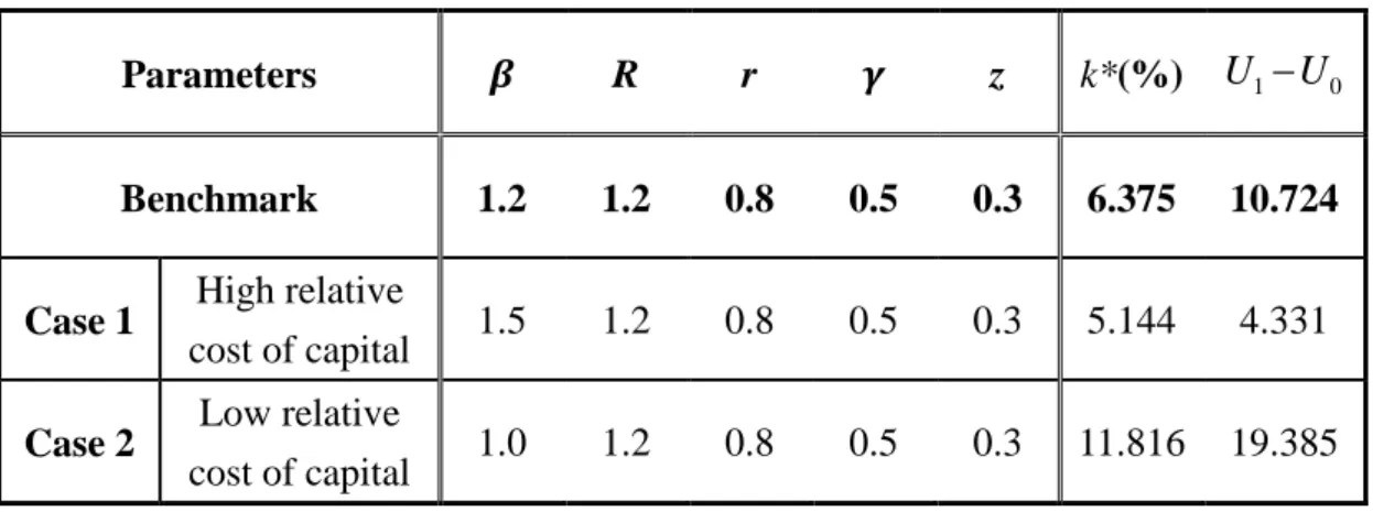
(34) TABLE 4 - Summary of Simulated Values of the Optimal k* R. r. 1.2. 1.2. 0.8. Parameters Benchmark. z. k*(%). U1  U 0. 0.5. 0.3. 6.375. 10.724. Case 1. High relative cost of capital. 1.5. 1.2. 0.8. 0.5. 0.3. 5.144. 4.331. Case 2. Low relative cost of capital. 1.0. 1.2. 0.8. 0.5. 0.3. 11.816. 19.385. Firstly, let’s check the results of our benchmark. With   1.2, R  1.2, r  1,. 政治大.   0.5 and z  0.3, we have the optimal level of capital requirement at 6.375%, which. 立. is quite a reasonable value. The social welfare has a gain of 10.724, showing the. ‧ 國. 學. benefit from the capital requirement. This result is important because it provides the government with a theoretical base for the capital regulation.. ‧. Secondly, we find that k* decreases when the cost of capital is higher R. 1.5  1.0  1.25 ) while it increases when the cost is lower (   0.83 ) relative to 1.2 R 1.2. y. . io. sit. . Nat. (. n. al. er. the benchmark; what’s more, the social welfare further increase with a higher k* at. Ch. i n U. v. 11.816%. This result is rational and shows that bank reduce the using of capital when. engchi. the cost is relatively high. Remember that from Proposition 3, we state that.  R.  1 is a. sufficient condition for the bank to increase buffer and lower the contagion possibility, which seems contradict to our conclusion here. Actually it is not. The result just highlights the fact that the bank will choose the cheaper way to finance itself. Also, the significant surge of the social welfare in case 2 (low cost of capital) indicates the great importance of the financial stability over the economy in our model. To be clear, after the optimization, the gains from financial stability exceed the loss of early consumption; hence, the region with higher level of capital requirement enjoys. 31.

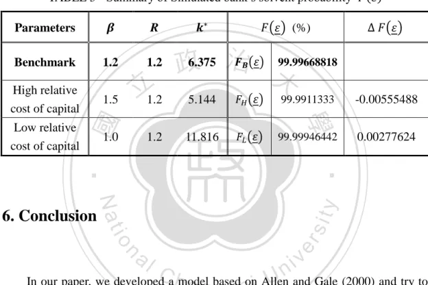
(35) higher social welfare, and vice versa for the bank with lower capital requirement. In addition, TABLE 5 reveals a notable point of solvency. We see that higher k* could raise. the, probability of bank’s. ; that is, higher capital requirement. rate could decrease the risk of bankruptcy, which is consistent with economic intuition. This consequence corresponds with Proposition 2.. TABLE 5 - Summary of Simulated bank’s solvent probability R. Parameters 1.2. 1.2. High relative cost of capital. 1.5. 立1.2. 1.0. 1.2. 99.99668818 政6.375 治大. 5.144. 99.9911333. 11.816. 99.99946442. 學. Low relative cost of capital. ‧ 國. Benchmark. (%). -0.00555488 0.00277624. ‧ y. Nat. er. io. sit. 6. Conclusion. al. n. v i n C U and Gale (2000) and try to In our paper, we developed ahmodel e n based g c honi Allen analyze the effectiveness of the capital requirement to the financial contagion phenomenon in the banking system. We find that, after the introduction of capital requirement, the capital structure of the bank has changed which affects the equilibrium consumptions and investment levels, and hence the possibility of bank runs. One important feature is that only as the return of equity owner. is larger than. the return of long asset investment R, the banks are willing to hold larger buffer to support the early withdrawals, and the spillover effect of the regional liquidity is also improved. However, by consider both the gain from the less possibility of banking. 32.

(36) crises and the loss of consumers (depositors) consumptions, we show that there exists an optimal capital level. to maximize the social welfare for the whole economy. (representative bank). By simulations, we find that the. is higher when the cost of. capital is relatively low, indicating the consideration of the price effect for the bank to finance itself. Finally, the social welfare increase with higher capital requirement rate, which emphasizes the gain of financial stability over the loss of early consumptions. This conclusion is consistent with our prior expectation. Our paper provides some important implications for the policy makers. Firstly,. 政治大 and financial contagion phenomenon in our model, which provide with a theoretical 立. we prove that the capital requirement can successfully reduce the risk of bankruptcy. fundamental for the policy maker to refer. Secondly, we formulate the optimal capital. ‧ 國. 學. requirement. as the function of different parameters, such as cost of capital ( ),. , and so on. The government can utilize this model. sit. y. Nat. bank’s solvency probability (. ‧. long term and short term asset return (R and r), probability of early withdraw ( ), the. io. er. to evaluate the degree of impact of the capital regulation by altering these parameters. Finally, the crucial conclusion about the positive relationship between k* and the. al. n. v i n C h of capital requirement social welfare highlight the effectiveness again, which support engchi U the current regulation from the Basel Accord.. However, there remain some space for future study and improvement. The Basel Accord requires the bank to hold capital based on a risk weighted basis of the portfolio, and they also consider different kind of risks such as credit risk, market risk and operational risk. In our model, for simplicity, we use a single k to represents the overall capital requirement among all the assets instead of setting different weight of asset x and y. The more complicated model is worth considering by adapting the above settings which match the reality more. The structure the financial linkage in our model is also of great interests. We showed that financial fragility only happen in the 33.

(37) incomplete market form and the capital requirement can effectively reduce the contagion, however, is the capital requirement still effective in other kind of market structure, such as the disconnected market? Finally, whether there exist other regulations methods such as deposit insurance that can also improve the financial fragility, or multiple methods can be implemented at the same time and achieve better performance? (both the prevention side and welfare side). These topics all need advanced study in the future.. 立. 政治大. ‧. ‧ 國. 學. n. er. io. sit. y. Nat. al. Ch. engchi. 34. i n U. v.

(38) 7. Appendix. Appendix A: Optimal risk sharing with capital requirement. Subject to: (A.1) (A.2). 立. 政治大. (A.3). ‧ 國. the function of. 學. From the constraints (A.1), (A.2) and (A.3), we rearrange and translate. into. , resulting the below equation.. ‧. (A.4). Nat. n. al. er. io. sit. y. Thus, we change the original problem into the new form without any constrain.. F.O.C.. Ch. engchi. i n U. , therefore, we have the optimal level of. v. as below.. (A.5) (A.6) (A.7) (A.8). 35.

(39) Appendix B: Effectiveness of k to Reduce Bankruptcy Probability. Follow the bankruptcy condition, we have the following inequality: , where. .Therefore,. we have that,. (B.1). .. Here. 政治大. represents the minimum excess liquidity demand that will trigger the. 立. bankruptcy of Bank A when there’s no capital requirement. Following the same logic,. ‧ 國. which is under capital requirement.. 學. where. ‧. io. sit. y. Nat. . Therefore, we have that,. n. al. er. we can calculate. Ch. Here we can exam that if let. engchi. i n U. v. , the result will just be the same as. (B.2). , and. this demonstrates our solution is correct. Our goal is to calculate the difference between. and. , namely,. , and see whether the minimum level of the. liquidity demand actually increases after the capital requirement is introduced, which means there is lower possibility for the bank to be bankrupt.. (B.3). 36.

(40) We reasonably assume that long asset. Obviously, if. for sufficient large return of the. , the denominator will be smaller and the numerator. will be larger, which makes the value of the ratio increase. However, we are still uncertain about the sign of the above solution. In order to figure out the net effect of the capital requirement, we take the partial derivative of. .. (B.4). 政治大. The above result is obvious positive without any conditions.. 立. Appendix C: Effectiveness of k to Reduce Spillover Effect. ‧ 國. 學. Recall the spillover condition (4.7) as follow:. ‧. ,. sit. n. al. er. io. and. y. Nat Substitute. into the complete form, we have:. Ch. engchi. i n U. v. (C.1). Before the capital requirement is introduced, we firstly calculate the SE by using. (C.2). After the capital requirement is introduced, we can define the spillover effect by using. 37.

(41) (C.3). Then we have the difference of the two the SEs.. (C.4). Obviously,. 政治大. is positive if the relative cost of capital. 立. for sufficiently large R). This means the spillover. 學. ‧ 國. assume that the term. (we reasonably. effect has been reduced successfully.. ‧. Appendix D: Derivation of Optimal Capital Requirement k*. sit. y. Nat. er. io. According to the equation (5.3), the process of optimization is shown as. a. v. n. . max k U  E u        lnlc1*C  1      ln(c2*   k )  nf i d  0. . . 1. h e n g c h i U .  ln c1  b      z  c1  q  *. . *. *. A*  .   . (D.1). f   d . where. c1*  (1  k . k R. ), c2*  R(1  k . k R. ), f ( ) . 1 , 1 . k     k 1    [1  k   R ]  b       r 1   1  k     , and R R     *. q. A*.   k  k   k     1  k   R  r  1   1  k   R )   z 1  k  R        1 z . 38.

(42) Let. and. denote the left-side and right-side terms, that is. . X . 0     ln c1  1      ln(c2   k )   f  d *.  ln c1  b      z  c1  q. 1. Y. *. . *. *. *. A*. (D.2).   f   d ,. (D.3). Also we let U  X  Y to represent the original welfare function, and then replace all the variables by the above values. To maximize the utility, we differentiate this function with respect to k, that is,. U X Y   k k k. 政治大. 立. ‧ 國. 學. By using Leibniz Differentiation Formula, we obtain. (D.4). 1   1  k  . R  1.  k R. .  B  r 1   1  k    k  R  ln  k B  r 1  k    R. . . .  B  r 1   1  k    k  R  ln  k B  r 1  k    R. . y. . sit.  . ). . al. n. r. R. er. . . io. k. . A  r 1   (1 . Nat. Y. ‧.            ln 1  k   k   1      ln R 1  k   k   1        X 1  1 R  R   2 2     R      1             k 2(1   )  1  k   k  1  1 k     R .    .  . . 1 1. Ch. en  g ch i 2. i n U. 1   (1  )   R     B  r 1   1  k    k   R. .   B   k   B  r 1   1  k     R. . where z  r  1  1 r 1    1   1   (1  )   R  R 1  z  R     2 k  r 1    R. 39. . . . v. . . . 2. B  r 1  k . . B. B  r 1  k . k R. k R. .     r .  .        ln  . . B 1 k . 1  k (1 . k R.  R. ). . .  0,.

(43) 1    1      k    1   (1   )  zR  1  r   1   (1   )          R  R  , and    A  R   R. 1     2. 1 z.     k   B  R  1   (1  )   r  1   1  k    ( R  1)  R   R  . For the first order condition, we have that. X Y   k k.  . kR  1   (1  1   .   ) R .  . zR 1  r   1   1  k   .  k  R.  . 1 z. U X Y    0 , therefore, k k k. 政治大.  1            ln  1  k   k   1      ln R  1  k   k  A  r  1   (1   )   R  1          1  2 2 R  R  R      R      1               k   k  2(1   ) 1   1 k  r  1   1  k    1  k       R  R   1. ‧ 國. 立. 2    1   (1   )  2     B   R        k  k   k      B  r  1   1  k    B  r 1  k   r 1  k   R  R    R     . 學.  B  r  1   1  k    k      1 R    ln   k  1     B  r 1  k    R    . ‧.  B  r  1   1  k    k           B B   R     ln       ln  1  k (1  )   0, D   k   k  k  R       B  r   1  k     B  r  1   1  k    B  r 1  k     R  R  R        . er. io. sit. y. Nat. Due to the complexity of the equation, we use simulation method for the parameters. al. n. v i n C h the optimal capital to calculate requirement k engchi U. such as. and. is discussed in Section 5.. *. 40. The process.

(44) 8. References Allen, Franklin, & Gale, Douglas. (1998). Optimal Financial Crises. Journal of Finance, 53(4), 1245-1284. Allen, Franklin, & Gale, Douglas. (2000). Financial contagion. Journal of Political Economy, 108(1), 1. Amil Dasgupta, “Financial Contagion through Capital Connections: A Model of the Origin and Spread of Bank Panics”, 2004, Journal of the European Economic Association, 2(6), pages 1049-1084.. 政治大 Solution for Capital and Liquidity", 2010, OECD Journal: Financial Market 立. Adrian Blundell-Wignall and Paul Atkinson, " Think beyond Basel III: Necessary. Trends, Volume 2010, Issue 1. ‧ 國. 學. Basel Committee on Banking Supervision, "Basel III: A global regulatory framework. sit. y. Nat. Settlements.. ‧. for more resilient banks and banking systems", 2010, Bank for International. io. er. Douglas W. Diamond; Philip H. Dybvig, "Bank Runs, Deposit Insurance, and Liquidity", 1983, The Journal of Political Economy, 91(3), page 401-419.. al. n. v i n Hellman, Murdock and Stiglitz,C “Liberalization, MoralUHazard in Banking, and hengchi. Prudential Regulation: Are Capital Requirements Enough?”, 2000, The American Economic Review, 90(1), page 147 - 65.. Jean-Charles Rochet, “Why Are there So Many Banking Crises?”, 2007, chapter 8, page 227-259. Patricia Jackon, “Capital Requirement and the Bank Behavior: The Impact of the Basel Accord”, 1999, Bank of International Settlement, Switzerland. Rafael Repullo, CEMFI and CEPR, "Capital Requirements, Market Power, andRisk-Taking in Banking", 2002, Journal of Economic Literature. Sangkyun Park, “The Bank Capital Requirement and Information Asymmetry”, 1994, 41.

(45) Federal Reserve Bank of St. Louis. Xavier Freixas, Jean-Charles Rochet, “Microeconomics of Banking” 2ed, 2000, chapter 9.4, page 319-328. Viral V. Acharaya and Tanju Yorulmazer, “Information Contagion and Bank Herding”, Journal of Money, Credit, and Banking, 2008, 40(1), page 215-231. Van den Heuvel, Skander J, "The welfare cost of bank capital requirements," 2008, Journal of Monetary Economics, Elsevier, vol. 55(2), pages 298-320. 立. 政治大. ‧. ‧ 國. 學. n. er. io. sit. y. Nat. al. Ch. engchi. 42. i n U. v.

(46)