An Energy-Aware, Cluster-Based Routing Algorithm
for Wireless Sensor Networks
JYH-HUEI CHANG
Department of Computer Science National Chiao Tung University
Hsinchu, 300 Taiwan
Cluster-based routing protocols have special advantages that help enhance both scal-ability and efficiency of the routing protocol. Likewise, finding the best way to arrange clustering so as to maximize the network’s lifetime is now an important research topic in the field of wireless sensor networks. In this paper, we present an Energy-Aware, Cluster- Based Routing Algorithm (ECRA) for wireless sensor networks to maximize the network’s lifetime. The ECRA selects some nodes as cluster-heads to construct Voronoi diagrams and rotates the cluster-head to balance the load in each cluster. A two-tier architecture (ECRA-2T) is also proposed to enhance the performance of the ECRA. The simulations show that both the ECRA-2T and ECRA algorithms outperform other routing schemes such as direct communication, static clustering, and LEACH. This strong performance stems from the fact that the ECRA and ECRA-2T rotate intra-cluster-heads to balance the load to all nodes in the sensor networks. The ECRA-2T also leverages the benefits of short transmission distances for most cluster-heads in the lower tier.
Keywords: sensor networks, energy aware, network lifetime, clustering, Voronoi diagram
1. INTRODUCTION
In recent years, the Micro-Electro-Mechanical Systems (MEMS) technologies have been booming. These MEMS technologies combined with advances in the wireless com-munication, make it possible to deploy low-cost, and low-power sensor networks. There are many civil and military applications of wireless sensor networks such as environmental monitors, informational gathers, battlefields monitors, and detectors of ambient conditions. The power for these sensor nodes comes from their batteries. Thus, finding the best use for the limited battery power is a crucial research issue in wireless sensor networks.
Many studies have focused on saving energy in different ways such as reducing the power spent on the modulation circuits [1], or managing the power usage on the MAC layer of sensor nodes [2, 3]. However, these schemes focused of the individual device, and that approach is too narrow when working with wireless sensor networks. Since sensor nodes have limited transmitting ranges, only a few nodes can communicate directly with the sink node. In most cases, the sensor nodes gather sensing data which must then be forwarded by the other node to the sink node. However, these cumbersome relaying opera-tions consume too much energy, thus causing the relay nodes to rapidly expend much of their power. Therefore, developing a load-balanced routing algorithm to maximize the network’s lifetime has become an important research topic.
A large number of routing protocols [4-10] for wireless sensor networks have been
proposed, but most are flawed in one way or another. In the fixed path schemes [4, 5], sensor nodes arrayed in a fixed path will consume much energy and get exhausted rapidly because they continually provide relaying service. The flooding scheme consumes too much energy for relaying duplicate packets. Source routing schemes [6, 7] solved some of the drawbacks of the flooding approach; however, they can not operate well when the number of hops between the source and sink is large. Energy-aware, multi-path routing schemes [8-10] have the advantage of sharing the energy among all the sensors in the wireless networks. Nevertheless, the chief disadvantage of multi-path routing schemes [8, 9] is that the sensor nodes only keep a local view of energy usage and the nodes in the network can not have an even traffic dispatch.
In addition, many studies have focused on cluster-based energy-efficient routing pro-tocol for wireless sensor networks [11-25]. Power-Efficient Gathering in Sensor Informa-tion Systems (PEGASIS) [11] prolongs the network lifetime with a chain topology. But the delay is significant although the energy is saved. Hybrid Energy-Efficient Distributed Clustering (HEED) [22] considers a hybrid of residual energy and communication cost when selecting cluster-head. A sensor has highest residual energy can become a cluster- head. However, if the residual energy of the sensors in a cluster is nearly the same, it takes many iterations and expends much energy to elect cluster-head. The Low Energy Adap-tive Clustering Hierarchy (LEACH) [23, 24] randomly selects some nodes as cluster- heads and rotates the cluster-head to distribute the load to all sensors in the wireless sen-sor networks. Its performance is better than that of the direct communication and static clustering routing protocols.
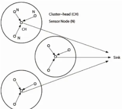
Fig. 1 shows an example of the cluster-based routing scheme for wireless sensor net-works. In Fig. 1, each cluster has one cluster-head. The non-cluster-head nodes transmit their sensing data to cluster-heads which then forward the aggregated data to the sink node. The use of clusters leverages the benefits of short transmission distances for most nodes. The cluster-head acts as a fusion point to aggregate the sensing data so that the amount of data that is actually transmitted to the sink node is reduced [23, 24]. Thus, network clus-tering can increase system lifetime and energy efficiency. Cluster-based routing protocols have special advantages: they can enhance the scalability and efficiency of the routing protocol to reduce the routing complexity [25], reduce the complexity of location man-agement [26], and improve the power control procedure [27].
However, LEACH may also have several problems: First, if the coverage of the ter-heads is too small, then some cluster-heads may not have any members in their clus-ters. Second, LEACH has a long transmission range between the cluster-heads and the sink node. Third, the LEACH requires global cluster-heads rotation. This cluster-head selection greatly increases processing and communication overhead, thereby consuming more energy.
Thus, this paper presents an energy-aware routing scheme, called an Energy-Aware Cluster-Based Routing Algorithm (ECRA), to overcome the LEACH’s problems and re-duce the overhead of cluster-heads rotation for cluster-based wireless sensor networks. The goal of ECRA is to maximize the network’s lifetime. The ECRA algorithm includes three phases: clustering, data transmission and intra-cluster-head rotation. In our work, we assume that the sensors are location-aware. The ECRA algorithm selects some nodes as cluster-heads to construct a Voronoi diagram. The sensor nodes transmit their sensing data to cluster-heads which forward the aggregated data to the sink node. Then, in the next round, ECRA chooses a sensor node from the previous cluster as a cluster-header, called an intra-cluster-head rotation. In this way, ECRA can balance the load for all sensors and avoid too many cluster-heads focusing on a small area. In addition, a two-tier architecture for ECRA, denoted as ECRA-2T, is proposed to enhance the performance of the original ECRA. The simulation results show that both ECRA-2T and ECRA outperform all other routing schemes: direct communication, static clustering, and LEACH. The system life-time of ECRA-2T is approximately 2.5 life-times than that of LEACH. ECRA-2T also requires much less energy consumption than that of direct communication. Simply put, the ECRA- 2T scheme shares the load evenly to all sensor nodes in the wireless sensor network and it has a longer lifetime. The ECRA-2T scheme also performs better than direct commu-nication and LEACH in terms of energy x delay. This advantage comes from the fact that the two-tier architecture leverages the benefits of short transmission distances for most cluster-heads in the lower tier.
The remainder of this paper is organized as follows. In section 2 we describe the en-ergy model of ECRA. Section 3 illustrates the details of the ECRA algorithm. The simula-tion results and performance analysis are shown in secsimula-tion 4. Finally, the conclusions are given in section 5.
2. ASSUMPTIONS AND ENERGY MODEL OF ECRA
In this paper we make the following assumptions: (1) All sensors are location aware. That is, they can convey their location information to the base station in the initialization phase (phase 0). (2) The base station has a power supply so we assume it has infinite en-ergy. Therefore, the energy required for the base station to inform each cluster-head can be ignored. (3) Base stations can compute the residual energy of all sensors in each round according to their location and the amount of transmission data.
The energy model of our study is the same as in [23]. In this energy model, the elec-tronic energy Eelec = 50 nJ/bit is needed to operate the transmitter or receiver circuit.
The transmitter amplifier is εamp = 100 pJ/bit/m2. Eqs. (1) and (2) are used to calculate
the transmission energy, denoted as ETx(k, d), required for a k bits message over a
ETx(k, d) = ETx_elec(k) + ETx_amp(k, d), (1)
= Eelec * k + εamp * k * d2. (2)
To receive this message, the energy required is:
ERx(k) = ERx_elec(k) = k * Eelec, (3)
where ETx_elec is the energy dissipation of transmitter electronics and ERx_elec is the energy
dissipation of receiver electronics. ETx_amp is the energy of the transmitter amplifier.
As-sume that ETx_elec = ERx_elec = Eelec. From Eq. (3), one can see that receiving data is also a
high overhead procedure. Thus, the number of transmission and receiving operations must be cut to reduce the energy dissipation. We also assume that the radio channel is symmetric such that the energy required to transmit a message from node i to node j is the same as the energy required to transmit a message from node j to node i for a given signal-to-noise ratio.
3. DETAILS OF THE ECRA ALGORITHM 3.1 Three Phases of ECRA
Our ECRA algorithm includes three phases: clustering, data transmission, and intra- cluster-head rotation. The details of the algorithm are given as follows.
Phase 1: Clustering
First, we define the Voronoi diagram and Centroidal Voronoi Tessellation (CVT) [28-30]. Consider an open set Ω ⊆ ℜ2
and a set of points {zi}in=1 belonging to Ω where Ω is the closed set of Ω. Let | . | denote the Euclidean norm in ℜ2
. The Voronoi region
Vi corresponding to the points zi is defined by
Vi = {x ∈ Ω | |x − zi| < |x − zj| for j = 1, …, n, j ≠ i} (4)
where Vi ∩ Vj = 0/ for i ≠ j and ∪in=1Vi = Ω.The set of {Vi}in=1 is a Voronoi diagram of Ω and each Vi is referred to as the Voronoi region corresponding to zi. The points {zi}in=1 are called generators.
CVT is a Voronoi tessellation whose generating points are the centroids of mass for their corresponding Voronoi regions. Formally, CVT can be defined as follows. Given a region Vi ⊆ ℜ2 and a density function ρ(x), defined in Vi, the mass centroid zi* of Vi is
defined by ( ) , for 1, , . ( ) i i V i V x x dx z i n x dx ρ ρ ∗=
∫
=∫
… (5)Given n points {zi}in=1, if the points zi = zi* for i = 1, …, n, then we call the Voronoi
tessellation defined by Eq. (4) as a CVT. That is, the points zi that serve as the generators
for Voronoi regions Vi are themselves the mass centroids of those regions. Fig. 2 shows
Fig. 2. The examples of CVTs for n = 2, 3, 4, 5. Fig. 3. Voronoi diagram of the 100-node random sensor network with centroidal points.
Fig. 4. Voronoi diagram of the 100-node random sensor network without centroidal points.
We apply the following two steps to partition the sensor nodes into n clusters. Step 1: Given sensing field Ω, a positive integer n, and a density function ρ(x) = c, con-struct a centroidal Voronoi tessellation such that Vi is the Voronoi region for zi* and zi* is
the mass centroid of Vi for each i. That is, the sensing field is partitioned into n Voronoi
regions.
Step 2: Let wi, i = 1, …, m, denote the sensor nodes in sensing field Ω.
(a) For each node wi, if wi ∈ Vj, then we assign node wi to cluster Cj.
(b) For each Cj, j = 1, …, n, find a sensor node wj* that is closest to zj*, the mass centroid
of Vj. Then, we choose sensor node wj* as the initial cluster head of cluster Cj.
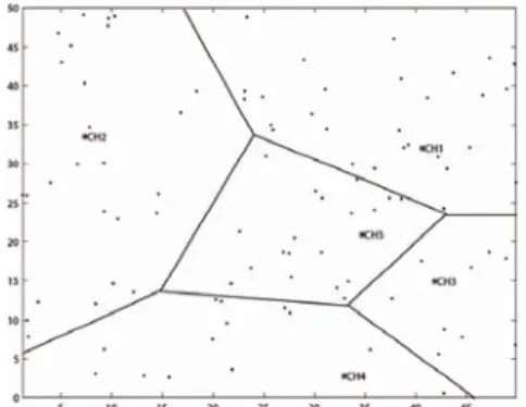
Fig. 3 shows that these cluster-heads are located nearest their corresponding cen-troidal points. The advantage of the above clustering method is that each cluster head has a nearly equal number of members. This is because the sensor nodes are uniformly distrib-uted. In contrast with Fig. 3, Fig. 4 shows the Voronoi diagram in which the generating points were selected randomly. Note that the clusters have diverse number of members.
In the ECRA scheme, we assume that the sensor nodes are location-aware. That is, the base station knows every sensor node’s location. The base station constructs CVT for
the sensing field. Each cluster has only one cluster-head. The base station tells each clus-ter-head which nodes are its member. The clusclus-ter-head broadcasts an advertisement to their members. By listening to the advertisement, each node knows which cluster it be-longs to. Then, the sensor node sends an acknowledgement to its cluster-head and con-firms that it will be a member of the cluster. During this time, all cluster-heads must re-main in active.
Phase 2: Data transmission
When the clusters are created, data transmission can begin. The nodes use single hops to communicate with their cluster-heads, and the cluster-heads communicate with the base station. Each node has M bits messages to transmit. The non-cluster-head node can be turned-off until its allocated transmission time in order to minimize energy usage. When all data from the nodes have been received, the cluster-head aggregates the total data into a single message to reduce the amount of information transmitted to the base station. Phase 3: Intra-cluster-head rotation
When a round is ended, next rotate the cluster-head within the same cluster based on a parameter called Oij which is a function of communication cost Edij and residual
energy Eniejw. The distance dij, i = 1, …, n, j = 1, …, |Ci| represents the distance from node
j in cluster Ci to the base station and is given as
2 2
( ) ( )
ij ij ij
d = x −x∗ + y −y∗ (6) where (xij, yij) is the position of node j in cluster Ci and (x*, y*) is the position of the base
station. The residual energy Eniejw is defined as
Eniejw = Eoiljd− Eeixjpend (7)
where Eoiljd is the residual energy of node j in cluster Ci at the beginning of the current
round. Eeixjpend is the energy expended by the node in the current round. Edij is the energy
expended by the cluster-head to transmit data to base station. Then, we define the pa-rameter Oij as , 1, , , 1, , | |. ij new ij ij i d E O i n j C E = = … = …
For each cluster Ci, we find
O(i) = max{Oij | j = 1, …, |Ci|}.
Node j in cluster Ci with the value of O(i) will become a cluster-head of cluster Ci at the
next round. That is, when all data are received in the current round, the base station first calculates the value of Oij for each node j in cluster Ci, then finds O(i) for each Ci, and
finally informs the node with value O(i) to become the new cluster-head at the next round. Note that the base station has the location of each node and it also knows that each sen-sor node has sent M bit messages, and thus the base station can calculate the value of Oij.
When the current round is ended, the role of the cluster-head will rotate to the node with value O(i) that is designated by the base station. Then, the new cluster-head begins to advertise using the method given in phase 1.
3.2 Enhancement of ECRA
The ECRA can be enhanced by adding an extra tier, called a high tier, on top of the original architecture (see Fig. 5). The high tier has only one cluster. All cluster-heads in the low tier are also the members in the high tier. This architecture is called a two-tier ECRA (denoted as ECRA-2T). The nodes in the high-tier forward their aggregated data to the node with the maximal remaining energy, called the main cluster-head.
(a) T. (b) T + d.
Fig. 5. The operation of high-tier architecture in enhanced ECRA, where T is the current round and
T + d is the next round, and so on.
The main cluster-head transmits the aggregated data to the sink. When a round is over, rotate the cluster-head of the low-tier in the sensing field based on the parameter Oij
(see Eq. (8)). The members of the high-tier in the next round consist of these cluster- heads. Fig. 5 illustrates the high-tier operation in ECRA-2T. In current round T, CH2 is the main cluster-head. In the next round, T + d, CH3 has a maximal remaining energy that is selected as the main cluster-head, and so on.
4. SIMULATION RESULTS 4.1 Performance Metrics and Environment Setup
This section presents the performance analysis of the ECRA algorithm. The per-formance metrics are given as follows.
(1) The lifetime for the first node to die (FND): FND is defined as the time required for the first node to run out of energy. The non-cluster-head nodes transmitted their
sens-ing data to the cluster-head. The cluster-heads forwarded their aggregated data to the sink periodically. We use the number of rounds to represent the network lifetime of FND. A round is defined as all nodes in the wireless network that finish returning their gathered data to the sink. The time interval between two rounds is assumed to be large enough for the last node to return its sensing data.
(2) The lifetime for the last node to die (LND): LND is defined as the time required for the last node to run out of energy, at which time the network crashed. We also use the number of rounds to represent the network lifetime of LND.
(3) The total energy dissipation (TED): This value is defined as the energy dissipation for all nodes that finish returning their gathered data.
(4) The cost of energy × delay: This value is the cost for each round of data gathering from sensor node to sink node. The energy cost can be calculated from the energy model described in section 2. The delay cost can be calculated as units of time. On a link with 2Mbps, a message of 2,000 bits can be transmitted in 1ms. Therefore, each unit of delay will be about 1ms for a sensor node with a single channel. We assume that the delay cost is 1 unit for each message of 2,000 bits transmitted.
We evaluate the performance of our study implemented with C++ and MATLAB. Four different sizes of deploying regions were simulated: 50 × 50 m2, 100 × 100 m2, 150 × 150 m2 and 200 × 200 m2. In each region, 100 nodes were deployed by uniform distribu-tion. Assume that the energy model is the same as in [23]. The electronics energy can be expressed as Eelec = 50 nJ/bit, εamp = 100 pJ/bit/m2. The energy of data aggregation is 5
nJ/bit/message. The cluster-heads use a 1-bit message to inform their members in each
round. Then, the members send their data to their cluster-heads. The negotiation energy consumption is included in each round. The sink node was located at the position ((x, y) = (25, − 100)). Each sensor has 2,000 bits of data sent to the base station during each round.
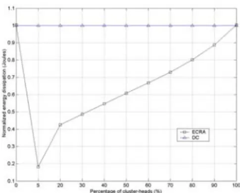
First, we determined the number of cluster head n. Note that if n is small, then the average length from sensor node to its cluster is large. This means that the energy costs between sensor node and cluster head is large. However, if n is large, then the total energy costs between cluster head and the base station is large. By simulation, Fig. 6 shows the normalized total energy dissipation related to different percentages of cluster-heads in ECRA. From Fig. 6 we learn that the normalized total energy dissipation is minimized at
Fig. 6. The normalized total energy dissipation related to different percentages of cluster-heads in ECRA.
5% of the total number of sensor nodes for ECRA. Thus, we chose n = 5 from 100 sensor nodes as cluster-heads.
4.2 Numerical Results
Comparisons of the four performance metrics were made for six schemes: the direct communication (DC), static clustering (SC), LEACH, PEGASIS [11], HEED [22], ECRA and ECRA-2T. The results are given as follows.
(1) The lifetime of FND under different initial energy levels: Fig. 7 shows that the lifetime of ECRA-2T in FND is better than LEACH, HEED, direct communication, and static clustering if the initial energy of each sensor is 1 J. Fig. 8 shows the lifetime of FND under different methods with different initial energy of each node. Overall, the life-time of FND increases when the initial energy of each sensor is greater. Both ECRA and ECRA-2T have better performance than other schemes. The lifetime of FND in ECRA-2T is approximately twice that of LEACH, but over eight times than that of direct communication and static clustering. That is, ECRA-2T gives better perform-ance than DC, SC, HEED and LEACH in the lifetime of FND.
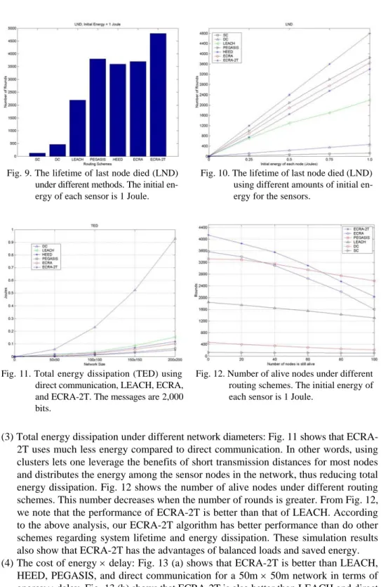
(2) The lifetime of LND under different initial energy levels: Fig. 9 shows that the life-time of ECRA-2T in LND is better than that of LEACH, HEED, PEGASIS, direct communication and static clustering if the initial energy of each sensor is 1 J. Fig. 10 shows the lifetime of LND under different methods with different initial en-ergy of each node. Overall, the lifetime of LND increases when the initial enen-ergy of each sensor is greater. Both ECRA and ECRA-2T have better performance than other schemes. The lifetime of LND in ECRA-2T is approximately 2.5 times longer than LEACH but over nine times greater than direct communication and static clustering. The results show that ECRA-2T gives better performance than DC, SC, PEGASIS, HEED and LEACH in the lifetime of LND. From Figs. 7 and 9, note that if a scheme shares the load evenly with all sensor nodes in the network, it can achieve a longer lifetime.
Fig. 7. The lifetime of first node died (FND)
under different methods. The initial en- ergy of each sensor is 1 Joule.
Fig. 8. The lifetime of first node died (FND) using different amounts of initial en-ergy for the sensors.
Fig. 9. The lifetime of last node died (LND)
under different methods. The initial en- ergy of each sensor is 1 Joule.
Fig. 10. The lifetime of last node died (LND) using different amounts of initial en-ergy for the sensors.
Fig. 11. Total energy dissipation (TED) using
direct communication, LEACH, ECRA, and ECRA-2T. The messages are 2,000 bits.
Fig. 12. Number of alive nodes under different routing schemes. The initial energy of each sensor is 1 Joule.
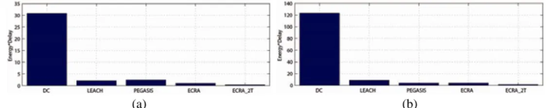
(3) Total energy dissipation under different network diameters: Fig. 11 shows that ECRA- 2T uses much less energy compared to direct communication. In other words, using clusters lets one leverage the benefits of short transmission distances for most nodes and distributes the energy among the sensor nodes in the network, thus reducing total energy dissipation. Fig. 12 shows the number of alive nodes under different routing schemes. This number decreases when the number of rounds is greater. From Fig. 12, we note that the performance of ECRA-2T is better than that of LEACH. According to the above analysis, our ECRA-2T algorithm has better performance than do other schemes regarding system lifetime and energy dissipation. These simulation results also show that ECRA-2T has the advantages of balanced loads and saved energy. (4) The cost of energy × delay: Fig. 13 (a) shows that ECRA-2T is better than LEACH,
HEED, PEGASIS, and direct communication for a 50m × 50m network in terms of energy × delay. Fig. 13 (b) shows that ECRA-2T is also better than LEACH and direct
communication for a 100m × 100m network in terms of energy × delay. This is be-cause the two-tier architecture leverages the benefits of short transmission distances for most cluster-heads in the low-tier.
(a) (b)
Fig. 13. (a) Energy × Delay cost for different routing schemes in a 50m × 50m network; (b) Energy × Delay cost for different routing schemes in a 100m × 100m network.
5. CONCLUSIONS
Cluster-based routing protocols have special advantages to enhance scalability and efficiency of the routing protocol. This paper presents an energy-aware cluster-based routing algorithm for wireless sensor networks. Compared with direct communication, static clustering, and LEACH, our ECRA-2T scheme can easily achieve longer lifetimes. This is because the ECRA-2T rotates intra-cluster-heads to balance the load to all nodes in the sensor networks. The CVT in clustering phase of our scheme is the key different from previous schemes. The CVT can achieve a better performance than other previous schemes. The numerical results also prove that ECRA-2T balances loads better and saves more energy than do other schemes. We are confident that ECRA-2T is an efficient and useful algorithm for further wireless ad hoc sensor networks.
REFERENCES
1. C. Chien, I. Elgorriaga, and C. McConaghy, “Low-power direct-sequence spread- spectrum modem architecture for distributed wireless sensor networks,” in
Proceed-ings of the 6th ACM International Symposium on Low Power Electronics and Design,
2003, pp. 251-254.
2. A. Sinha and A. Chandrakasan, “Dynamic power management in wireless sensor networks,” IEEE Design and Test of Computers, Vol. 8, 2001, pp. 62-74.
3. Y. Wei, J. Heideman, and D. Estrin, “An energy-efficient MAC protocol for wireless sensor networks,” in Proceedings of the 21st Annual Joint Conference of the IEEE
Computer and Communications Societies, 2000, pp. 1567-1576.
4. J. Moy, “OSPF version 2,” RFC 2178, Internet Engineering Task Force, 1997. 5. J. Moy, OSPF: Anatomy of an Internet Routing Protocol, Addison-Wesley, Boston,
1998.
6. A. Boukerche, X. Cheng, and J. Linus “Energy-aware data-centric routing in micro- sensor networks,” in Proceedings of the 6th ACM International Workshop on
Model-ing Analysis and Simulation of Wireless and Mobile Systems, 2003, pp. 459-468.
networks,” in Proceedings of Wireless Communications and Networking Conference, 2001, pp. 1028-1037.
8. X. Hong, M. Gerla, R. Bagrodia, J. K. Taek, P. Estabrook, and P. Guangy, “The mars sensor network: efficient, power aware communications,” in Proceedings of Military
Communications Conferences, 2001, pp. 418-422.
9. X. Hong, M. Gerla, W. Hanbiao, and L. Clare, “Load balanced, energy-aware com-munications for mars sensor networks,” in Proceedings of IEEE Aerospace
Confer-ence, 2002, pp. 1109-1115.
10. K. Sohrabi and J. Pottie, “Protocols for self-organization of a wireless sensor net-work,” IEEE Personal Communications, Vol. 7, 2000, pp. 16-27.
11. S. Lindsey and C. Raghavendra, “PEGASIS: Power-efficient gathering in sensor information systems,” in Proceedings of IEEE Aerospace Conference, Vol. 3, 2002, pp. 1125-1130.
12. W. R. Heinzelman, J. Kulik, and H. Balakrishnan, “Adaptive protocols for informa-tion disseminainforma-tion in wireless sensor networks,” in Proceedings of the ACM
Mobi-Com, 1999, pp. 174-185.
13. J. Kulik, W. R. Heinzelman, and H. Balakrishnan, “Negotiation-based protocols for disseminating information in wireless sensor networks,” Wireless Networks, 2002, pp. 521-534.
14. C. Chiasserini, I. Chlamtac, P. Monti, and A. Nucci, “An energy-efficient method for nodes assignment in cluster-based ad hoc networks,” ACM Wireless Networks, Vol. 5, 2004, pp. 223-231.
15. S. Bandyopadhyay and E. J. Coyle, “An energy efficient hierarchical clustering al-gorithm for wireless sensor networks,” in Proceedings of IEEE INFOCOM, Vol. 3, 2003, pp. 1713-1723.
16. M. Younis, M. Youssef, and K. Arisha, “Energy-aware routing in cluster-based sen-sor networks,” in Proceedings of the 10th IEEE International Symposium on Modeling,
Analysis, and Simulation of Computer and Telecommunications Systems, 2002, pp.
129-136.
17. V. Mhatre and C. Rosenberg, “Homogeneous vs. homogeneous clustered sensor net-works: a comparative study,” in Proceedings of IEEE International Conference on
Communications, 2004, pp. 3646-3651.
18. A. A. Abbasi and M. Younis “A survey on clustering algorithms for wireless sensor networks” Computer Communications, 2007, pp. 2826-2841.
19. J. Yick, B. Mukherjee, and D. Ghosal, “Wireless sensor network survey” Computer
Networks, Vol. 52, 2008, pp. 660-669.
20. S. Basagni, “Distributed clustering algorithm for ad hoc networks,” in Proceedings of
the International Symposium on Parallel Architectures Algorithms and Networks,
1999, pp. 310-315.
21. H. Chan and A. Perrig, “ACE: An emergent algorithm for highly uniform cluster for-mation,” in Proceedings of the 1st European Workshop on Sensor Networks, 2004, pp. 154-171.
22. O. Younis and S. Fahmy, “HEED: A hybrid, energy-efficient, distributed clustering approach for ad-hoc sensor networks,” IEEE Transactions on Mobile Computing, Vol. 3, 2004, pp. 660-669.
com-munication protocol for wireless microsensor networks,” in Proceedings of the 33rd
Hawaii International Conference on System Sciences, 2000, pp. 1-10.
24. W. R. Heinzelman, A. Chandrakasan, and H. Balakrishnan, “An application-specific protocol architecture for wireless microsensor networks,” IEEE Transactions on
Wireless Communications, Vol. 1, 2002, pp. 660-669.
25. A. Iwata, C. C. Chiang, G. Pei, M. Gerla, and T. W. Chen, “Scalable routing strate-gies for ad hoc wireless networks,” IEEE Journal on Selected Areas in
Communica-tions, Vol. 17, 1999, pp. 1369-1379.
26. W. Chen, N. Jain, and S. Singh, “ANMP: ad hoc network management protocol,”
IEEE Journal on Selected Areas in Communications, Vol. 17, 1999, pp. 1506-1531.
27. T. Kwon and M. Gerla, “Clustering with power control,” in Proceedings of Military
Communications Conferences, 1999, pp. 1424-1428.
28. K. Mulmuley, Computational Geometry, Prentice Hall, Englewood Cliffs, NJ, 1994. 29. F. Aurenhammer, “Voronoi diagrams − A survey of a fundamental geometric data
structure,” ACM Computing Surveys, Vol. 23, 1991, pp. 345-405.
30. Q. Du, V. Faber, and M. Gunzburger, “Centroidal Voronoi tessellations: applications and algorithms,” Society for Industrial and Applied Mathematics Review, Vol. 41, 1999, pp. 637-676.
Jyh-Huei Chang (張志輝) received his M.S. degree in Computer Science from National Chiao Tung University, Taiwan in 2002. He is currently working toward the Ph.D. degree in Com-puter Science at National Chiao Tung University, Taiwan. He is a Ph.D. candidate now. His research interests include wireless net-works, wireless sensor networks and mobile computing.