Integral variable structure control of nonlinear system using CMAC-based learning approach

Proceedings of the American Control Conference Anchorage, AK May 8-1 0,2002

Integral Variable Structure Control of Nonlinear System Using CMAC-based Learning Approach

Wei-Song Lin' and Chin-Pao Hung'.'

'Institute of Electrical Engineering National Taiwan University

Taipei, Taiwan, R.0.C

*

Department of Electrical Engineering Taichung, Taiwan, R. 0. C. National Chin-Yi Institute of Technology E-mail: cbhong@chinyi.ncit.edu.tw

Abstract

A CMAC-based controller with a compensating neural network and an update rule is proposed to design the integral variable structure control (IVSC) of nonlinear system. The control scheme comprises a stabilizer controller and a CMAC neural network. Based on the Lyupunov theorem, the stabilizer controller guarantees the global stability of the system. The CMAC neural network performs the equivalent control by a real-time learning algorithm. The proposed control scheme is globally stable in the sense that all signals involved are bounded. The new IVSC control scheme reduced the dependency to system parameters. Simulation results of numerical example demonstrate the effectiveness and robustness of the proposed controller.

Keywords: integral variable structure control, CMAC, nonlinear system, neural network control, leaming control, sliding mode,

vsc

1.

Introduction

Dr. Chern first proposed the integral variable structure control (IVSC) to solve the steady state error problem, and to improve the robustness of traditional variable structure control (VSC) in 1991[1]. Then Chem applied this control scheme to robot manipulator [2], brushless DC servo system [3-4][8], DC motor [5], and induction motor [6][9][11], to demonstrate the feasibility of IVSC. The related researchers also proposed a new design method for IVSC [7]. Other applications are such as the engine system [lo], the UPS

system [ 131, and the voltage regulator system [ 121. Since the IVSC introduced the integral state variable into the controller design, it can solve the steady state error problem of conventional VSC because of the dead zone or the boundary layer [ 14-15]. However, regardless of either the traditional VSC or the IVSC scheme, the controller design is

a parametic scheme that more dependent on the system model or parameters.

In the past year, the authors developed a real time leaming scheme to solve the VSC design problem of unknown parameters dc servo system 1161. In [16], we introduced a CMAC [17] neural network into the VSC. The CMAC, in a table look-up fashion, produced a vector output in response to a state vector input. It is like the models of human memory, using local data to perform reflexive processing. Fig. 1 shows a schematic diagram of CMAC network, through a serious of mapping every input state x map to produce an output y [18]. The mapping processes

satisfy the similar inputs excite similar memory addresses, i.e. if the input states are close in input space will have their corresponding sets of association cells overlap. For example, if x I and x2 are similar (close), X I excites the memory addresses al,u2,u3,a4, x2 should excite the memory addresses a2,a3,a4,a5 or a3,a4,a5,a6..

If

two inputs fire up the same memory addresses, we say the similarity of the two inputs is high. Low similarity would active fewer same memory addresses. If the reference input state is a smooth function, every adjacent state can be thought of as similar inputs (with proper quantization level width). Assuming similar input command should have similar control force, the characteristic of local reflexive action makes CMAC attractive to on line application in control system.

In this paper we expand the control scheme to the IVSC

of

nonlinear system and improve the learning law to demonstrate why the CMAC can work well. In this new IVSC structure, the controller design only needs little model information. Based on the Lyapunov theorem, a stabilizer controller guarantees the system stable running. The e CMAC neural network with learning algorithm approximates and performs the equivalent control depending on the uncertainties and the constraints of the desired integral sliding surface. This is unlike the conventional parametric methods in that equivalent control is obtained from the nominal model assume free uncertainty. With application of this scheme to a nonlinear system, computer simulations demonstrate the success of the proposed method.

2. Problem formulation

Consider the n-order nonlinear systems of the form [ 191

where f is an unknown continuous function, b is a positive unknown constant, and U

E R

and y E

R

are the input and output of the system, respectively. We assume that the state vector g = (xl ,x2,. .xn) =(x,x,-. . , x ( ~ ' ) ) ' ER" is available for measurement. Therefore, the control objective of this paper can be described as follows:

Determine a feedback control U(&)@ and a leaming law for adjusting the vector _ ~ = ( ~ q , w ~ ; ~ . w , ) ' ~ R ~ l , g is the selected memory size, such that the following conditions are met:

1) The closed loop system must be globally stable in the sense that all variables, x_(t).w(t) and u(gld, must be uniformly bounded; i.e., In_(t)lI MX<q IE(t)l I

M,<ca

and

lu(x1~)I IMu<co, Ms, M,, Mu are design parameters specified x'") = f(x,X

,...,

x'"-'))

+

bu ,

y = x (1)

by the designer.

2) The tracking error e=ycy, should be as small as possible under constraints in 1) and

xd

=(yd,yd;..,yd

(n-1))T

,

e=(~t..;k"'))T=(~,q,..;%)Tand

k

=

(k,,...kl)T

E R "

be such that all roots of the polynomial h(s) = s"

k,

are in the open left-half plane. Here,

k,,i

= 1, n are designed to satisfy the IVSC sliding surface function defined as following [ 13 klsn n K , Z

+

c , e l 0 (2) Z = y d - x l = e (3) C, =l,c,

,

= k i , i =l;..n l , k ,

K ,

(4) 1 1 and

3.The CMAC-based integral variable structure control 3.1 The structure of proposed controller

known (CIVSC)

As described above, if the exact system model is

. K , Z

+

c l e f 0 ( 5 ) K , ( y , - x I )

+

c,e,+,

+

( Y , ' ~ '

-

x'")) 0 ( 6 ) K , e ,

+

c,e,+l + y , ' " ) -

f(x)

- bu 0

(7)

I I n - l , I n - l I I

Then the optimal equivalent contr

where k = ( k , , . . . k , ) T = ( K , , c

,,...,

c, results in Applied(8) to(1) x(") = f ( x ) - f ( x ) y d f n )

/&)

i.e. e(,) + k l e ( "

+...+

k , e = O (9) which implies that lime(t) 0

,

the main objective is achieved. Since

f

and b are not exactly known, the optimal equivalent control cannot be implemented. Our purpose is to design an IVSC controller using CMAC-based learnirg approach to approximate the optimal equivalent control U

.

CMAC control uN

(x

1

2) and a stabilizer control U,

(x)

:

Substituting (10) into (l), we have

Now adding and subtracting b(f,Ju' to (1 1) and after some

t+

Suppose the control U ( X

1

E) is the summation of a

U(X

I

E) = U N

(x

I

E) + U , W (10)

dn)

=

f(x)

b[u,(x 12) U,(X)l (11)

straightforward manipulation we obtain the following error equation goveming the closed-loop system:

or, equivalently,

where

e(,)

=+'e

b[u* - v N ( ~ ( w ) - u S ( x ) ] (12)

k Ace

+ - U N

(x

1

w)

-

U,

(x)]

(13) [ O 1

o

0.-

01

pi

.

.bc=

l o

: 0 0 1

o...

0 A c =

I:

.

1 - k ,

-k,

- k l J IbJ Define V,

definite matrix satisfy the kyapunov equation

where P O is specified by designer.

Using (15) and the error equation (1 3), we have

O.SgTPg, where P is a symmetric positive

AT,P+ PA, = Q (15)

V, O.StjTPg

+

0.5g"Pg (16)

1

= 0.5 Acg + ecru' u N Q 1 E) u,Q)])TPg + 7g'P Acg + kc[u' U& I?) I&)]] -0.5gTQg+grP~,[u* -iaN(x l w ) - u s ( z ) ]

4 0.5eTQg+

I

g T P ~ ,

II*H

[ U i- un(xlw)l gTPbcu,(x)l (17) Our task now is to design U, such that

V,

I 0 . In order to do

so, we need the following assumption:

Assumption 1: We can determine a fimctionf'($ and a constant bL such that f(iJI srfu(x) and O<bL 2 b.

Therefore, substituting (8) into (17) we construct the U,

as

follows:

_ -

where Zl* = I , if V,

designer) and 1; = 0, if V, 5

Considering the 1; = 1 case, substituting (18) and (15) into (1 7) we have

V ( V is a constant specified by the

.

Therefore, using the supervisory control U,, we always have

V,

I

v .

Because DO, the boundedness of V, implies the

boundedness of

e,

which in

turn

implies the boundedness of g. From (18) U, is nonzero only when the error state is greater than specified value. That is, if the CMAC is well behaved, the U, is zero to avoid the control signal being too large.

3.2 Learning process vector 411.

Define the optimal weighting vector [ 191:

-

w *

argmin

(20)

E U N ( X ~ W 4 ) (21)

and the minimum approximation error:

The CMAC output is described as [ 2 3 ]

where ( 5 ) R' is the mapping function

of

CMAC network. Note that the

~ ( d

only contains the elements of 0

and 1. The numbers of 1 are equal to the numbers of fired memory cells A' and thenL(X)I

Then the error equation (13) can be rewritten as

U N

(x

I

E) =

Jx)w

( 2 2 )

-

U .

i

= A , E + b , l U N ( X

I

E*) UN(&

I

E91

b,u,(x)

b,

=

&e

+

b,

&)

btu,

(z)

b,

( 2 3 )

where =E* E.

Define the Lyapunov function candidate

-

1 bA* T

V = - - e T P q

-

2 - 2 p -

-

the following theorem guarantees the properties of the proposed control scheme.

Theorem 1: Consider the nonlinear plant (1) with the control (lo), where u,d&) is the CMAC output and U,& is given by (18). Let the weighting vector be updated by the learning law ( 3 0 ) and let the assumption 1 be true. Then, the overall control scheme guarantees the following properties.

and

L J

for all t 2 0 , where is the minimum eigenvalue of P (34) I 2 1 2 2 .

_,

_I

e(r)l d r 5 a

+

c

I<(r)l

d r , 0 where have

is a Positive constant. Using ( 2 4 ) and (1719 we _{for all t 2 0, where a and c are constants, and is defined} by

(2

1 ).

1 T T bA* p

2 -

V=---e @ + g P b c ( p ( x ) - u , - C ) + - ( 2 5 ) 3 . If is squared integrable, i.e.

I

(r)12dt < , then

P - -

0

- -

let

en

be the last column of P; then from (14) we have _{Iim,+ k(t>l= 0 .}

i) To p r o v e k t 5 M,, we let V , =0.5_wT_w. If the first line of (30) is true, we have either

hl5

M , or

"

Pn 'w

-

I O w h e n W = M ,

,

it is clear that we T

e r p i ,

e

p , b ( 2 6 ) Proof:

Substituting ( 2 6 ) into ( 2 5 ) ,

1

and using the fact

Ax_)

(5)

= T ( x ) p T ( x ) a n d (sincep R' g,

R g

'

1,

we have T

-

-

-

-

-

-

I b 2 - p - V = -e'Qe_+-#' / ? e _ ' ~ , ~ ~ ( , x ) + A ' d g'Pb,u, grPb, (27) ' W =-' A*

-

Since

_-

= -E, therefore, if we choose the learning law as have

kl

'

M w . If the second line is we have

bI

=

M,

and

follows:

then (27) becomes Therefore we always have

always have

v,

5

v .

Therefore,

I M cI, ,Vt 2 0

.

As described above, using the supervisor control

_-

U , , , we

(29)

best we can achieve. Fortunately, assume the memory size is

to zero. A large enough Q matrix will easily have V 0

.

T V

I

-0.5gTQg

-e

Pb,

where we use the fact gTPb,tr, 2 0 (cf.(18)). This is the large enough the CMAC can approximate function to arbitrarily accurate [ 2 3 ] . The second term

of

(29) will tend

2 7

)%

( 3 5 )

-

1 2

-

_{$ ' ~ g V , i.e.}

_kl

_(--- 2 min 2 v Since< ~ ~ -we h a v e k l i - k d I 2 , k \ 5 1 i d l

(-1

,

In order to guarantee the 5 M,,., we modify the mm

leaming law as which is (32). Finally, we prove

(33).

Since,

-(&)E is only the sum of fired memory cells, =

$A

kl

I

$A

M , , .

fPe'pP&T(g

. U,,,(&

I

E)

we have

luN(x

1

_w)I

I

I (&)lbl

ii) From (27), ( 3 0 ) , we have

,4.

.

if

14

< A(,

or14

= .M, andg'p _ n - w r - '(E) i 0

(30)

I ( = (

- p & - Q I ) I <,

if14

= M, a n d ~ ~ e ~ ~ ' - ~ ( ~ ) > 0

I I ,4' J Therefore, from (10) and (18), we have (33).

where 11=0(1) if the first (second) line of (30) is true. Now we will show that the last term of (36) is nonpositive. If 11=0, the conclusion is trivial. If II=1, which means that

bI

M,

a n d g T

p,_w

T

-

T

(x)

0 . S i n c e W = M ,

w'

,

therefore the last term of (36) is nonpositive, and we have

(37) 1

2 -

V < -eT& gTPb,u, gTPb,

As described above, gTPb,u, 2 0 ; therefore, (37) can be

further simplified to

1

where Qmln is the minimu eigenvalue of Q. Integrating

both side of (38) and selecting that Q m i n 1 (we can choose such a Q to satisfy this condition), we hbve

7

and 2

Define a=- IV(O>l SUPt

o p ( 0 J

c = - IPb,r

,

then (39) becomes (34).

Q m i n -

Q m i n -

iii)lf ( I )

L,,

then from (34) we have g L , , since all the variable of the right-hand side of (23) are bounded, we have

2

L

,

using Barbalat's lemma, we have

lim,+ k(t)l= 0 . Q.E.D.

Remark 1: For real control system, the state x_ and control force U are required to be constrained within a certain region.

Such as the robot system, the joint positions are constrained within workspace and the control signal should be smaller or equal to the output of the computer interface card. Depending on the practical constrain, the designer specified M, and

Mu.

Then based on (33) and (34) the sliding surface,

M,,

Q, and

V

can be chosen to satisfy the required performance and let the state x_ and control force U be within

the constraint sets.

3.3 Control algorithm

The structure of the proposed scheme is shown in Fig. 2 and the control algorithm is summarized as follows: Step 1. Specify the design parameters Mx,

M u

based on

practical constraints.

Step

2.

Specify the integral sliding surface function ad,

kf,,

Q and

y ,

based on (33) and (34). And using Matlab

lyap() and eig() functions to solve the P matrix,

Step 3. Transform the sliding surface to the desired error Step 4. Send the desired next error states ~ ( t ) to the CMAC Step 5 . Perform a series of mappings to transform the input Step 6. Calculate the stabilizcr control signal u,(t).

Step 7. The uN(t) is assumed to be an optimal equivalent control signal and is added to the output of the u,(t) to form the control signal U(?).

Step 8. Send U($ to plant to produce the actual output states

e, (t)

.

Step 9. Calculate the values of the actual error state

e.

Step 10. Update the fired weights using equation (30). Step 11. If t

and

Qmin '

states for the next control cycle

od

( t ) 3 g d ( t )

.

network.

values to the CMAC output uN(t).

T

, stop.

( T

is the control cycle.) Otherwise, Noted that the step 1 to step 3 are off-line processes and others are on line computing. Th,e related parameters of CMAC, quantization levels and A

,

are also specified off line. They can be adjusted depending on the weighting distribution plot.

4. Numerical example

as following [ 161: go to step

3.

Considering a simplified. robot system model described

(40)

XI ( t ) = x2 ( t )

x2(f) =Oxl -(33 5sint)x2 (300 50sint)u where

x,

=

x

is the end-effector output. Define the error output

_e

₌

_{y ,}

_-

_x

_e,,

_{6, e2}

.

y ,

is the desired end-effector output. Without lose of generality, we let

Y ,

=1 .We choose the integral sliding surface as following: = K ,

e,&

c,e,

e 2 ,

K ,

= l,c, = 10 (41) i.e.

k

= [l 101

.

In equation (15) the design parameters Q is given by Q = 101,

.

The P matrix can be obtained easily using the Matlab lyap( ) function. The associated design parameters of CMAC network are list as follows:

y ,

=l,quantization level 30, memory size 4096, fired memory cells

A*=lO,M,=!j(rad),Mu=lO(volt),

Mw=2,

v

=1, and P =

[

]

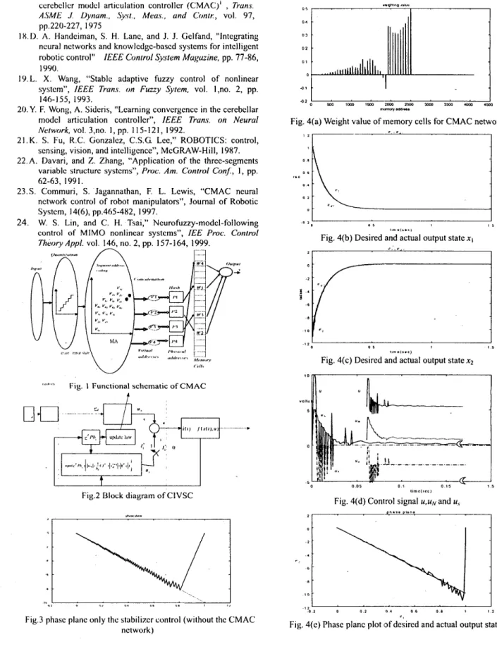
.Fig. 3 shows the phase plane output only the stabilizer controller. Introducing the CMAC network into the system (shown as Fig. 2), the simulation results are shown in Fig. 4. Fig.4 (a) shows the weighting values of the memory cells. Fig.4 (b)(c') are the error output, it is clear that the new CIVSC approach can give an almost accurate

servo

tracking response to partial known parameters system. Figs. 4(d) shows the wavef'orms of control functions, and we p=0.8,bL=250,

f u

= 38.1~21

,

emin

= l o , ,,,in =OS049

51 - 5 - 5 1

see

that the

CMAC

outputs are dominant gradually. Fig. 4(e), the phase plane plot, also shows the output nearly tracks the integral sliding surface.

Remark 2: The selection of M ,

M u

and

M ,

are dependent on practical constraints. M, and

Mu

represent the maximum rotated angle of robot arm and the maximum control signal

of the D/A card output. It is easy to specify as 5 rad and

10

volt. Using (33) we let the

M i

=2. The control result of Fig. 4(a) shows

CWI

1.226 that is smaller than

M,.

5. Discussion

In FigA(e) we see that the trajectory vibrated in the neighborhood of hitting point. Before the trajectory hit the sliding surface, the leaming is blind. It is easy to cause over tuning and give rise to the chattering. We wish the leaming behavior happened in the neighborhood of the desired surface, therefore using multiple segments sliding surface is better than only one sliding surface. But related sliding surfaces design and leaming law proof are under studying.

The stabilizer control just to preserves the output states near the sliding surface, the switching gain depends on the parameters bounds should be chosen carefully. Too large switching gain is easy to cause vibration. Fortunately, the stabilizer control is only active when some special conditions exist. In Fig.4(d) we see that U, is equal to zero for most time.

The training gain is related to the leaming effect. In generally, the value of is between 0 and 1 for supervised leaming

[18],

i.e. O< 1. The memory size of CMAC also affects the control performance. The memory size depends on the desired input signal and the performance requirement It is hard to make a clear decision but

we

can obtain some idea from the activity of memory address. For example, the weighting value distribution plot (Fig. 4(a)) shows that not all the addresses excited, in this case the memory size is enough. We can reduce the quantization level or association cells number to decrease the memory size. On the other hand, if all the addresses have been excited, the memory size may be not enough. We need to adjust the quantization level or association cells number to increase the memory size. When the memory size is too large beyond the computer specification, the Hash coding is needed.

6. Conclusion

In this paper, a new integral variable structure control scheme is proposed to control the nonlinear system. A CMAC network is used to leam the equivalent control of

CIVSC for the partial known system model. A stabilizer controller based on Lyapunov synthesis approach is designed to guarantee the stability of the proposed scheme in the sense that all signals involved are uniformly bounded. This CIVSC scheme only used little model information to design the contfoller. Using the generalization property

of

neural network, the CMAC can leam the approximated equivalent control signal on line and yield a robust sliding mode control. It can keep all the advantages of IVSC and alleviate the dependency to system parameters. Applying this scheme to a simplified robot manipulator model, it can

produce an integral variable structure control signal for specified sliding surface. The simulation results demonstrate the success of the proposed scheme.

6. Reference

1. T. L. Chem, Y. C. Wu,” Design of integral variable structure controller and application to electrohydraulic velocity servosystems”, IEE Proc. D vol. 138, no. 5, pp. 439-444, 1991.

2. T. L. Chem, Y. C. Wu,” Integral variable structure control approach for robot manipulator”, IEE Proc. D vol. 139, no. 2, 3. T. L. Chem, Y. C. Wu,” Design of brushless DC position servo

systems using integral variable structure approach”, IEE Proc. Bvol. 140, no. 1, pp. 27-34, 1993.

4. S. K. Chung, J. H. Lee, J. S. KO, M. J. Youn,” Robust speed control of brushless direct-driver motor using integral variable structure control”, IEE Proc. Elect,: Power Appl.,

vol. 142, no. 6, pp. 361-370, 1995.

5. T. L. Chem, J. S. Wong,” DSP based integral variable structure control for DC motor servo drivers”, IEE Proc. Control Theory Appl. vol. 142, no. 5, pp. 444-450, 1995.

6. T. L. Chem, C. S Liu, C. E Jong, and G M Yan, “Discrete integral variable structure model following control for induction motor drivers”, IEE Proceedings-Electric Power Applications, vol. 143, no. 6, Nov., pp. 467-474, 1996. 7. J. D. Wang, T. L. Lee, Y. T. Juang,” New methods to design an

integral variable structure controller”, IEEE Trans. Automation Control, vol. 41, no. 1, pp. 140-143, 1996. 8. T. L. Chem, J. Chang, G K. Chanf,” DSP based integral

variable structure model following control for brushless DC motor drivers”, IEEE Trans. Power Electronics, vol. 12, no. 1, 9. T. L. Chern, J. Chang, ” DSP based induction motor drivers

using integral variable structure model following control approach”, IEEE Trans. Power Electronics, vol. 12, no. 1, pp. 10.T. L. Chem, C. W Chuang, “Design of optimal MIMO DIVSC systems and its application to idle speed control of spark ignition engine”, ASME Journal of Dynamic Systems Measurement and Control, vol. 119, June, pp.175-182, 1997. 11 .T. L. Chem, J. Chang, K. L. Tsai, “IVSC-based Adaptive Speed

Estimator and Resistance Identifier for an Induction Motor”, Intemational Journal of Control, vol. 69, no. 1, pp.31-47, 1998.

12.T. L. Chem, G K. Chang, “Automatic voltage regulator design by modified discrete integral variable structure model following control”, Automatica, pp. 1575-1 582, 1998. 13.T. L. Chem, J. Chang, C. H. Chern, H. T. Su,

”Microprocessor-based Modified Discrete Integral Variable Structure Control for UPS,” IEEE Trans. Industrial Electronics, Apirl, 1999.

14.K. K. D. Young, ” Controller design for a manipulator using

theory of variable structure systems”, IEEE Trans. Syst., Man, Cybern. ,vol. SMC-8, no. 2, pp.101-109, 1978.

15.J. J. Slotine, S. S. Sastry, Tracking control of nonlinear systems using sliding surface, with application to robot manipulators , INI: J. Control, v01.38, no. 2 , pp. 465-492, 1983.

16. W. S. Lin, C. P. Hung,” Variable structure control of unknown parameter dc servo systems using CMAC-based leaming approach”, Proc. Am. Control ConJ, 2001.

pp. 161-166, 1992.

pp. 53-63, 1997.

53-63, 1997.

cercbellcr model articulation controller (CMAC)' , Truns.

ASME J. Dynum.. Sy.st.. Meus.. and C b n t ~ , vol. 97, pp.220-227, 1975

1X.D. A. Handeiman, S. H. Lane, and J. J. Gelfand, "integrating

neural networks and knowledge-based systems for intelligent robotic control" IEEE Control System Muguzine, pp. 77-86, 1990.

19.L. X. Wang, "Stable adaptive fuzzy control of nonlinear system", IEEE Trans. on Fuzzy Sytem, vol. 1,no. 2, pp. 20. Y. F. Wong, A. Sidcris, "Learning convergence in the cerebellar modcl articulation controller", IEEE Truns. on Neural Network, vol. 3,no. 1,pp. 115-121, 1992.

21.K. S. Fu, R.C. Gonzalez, C.S.G Lee," ROBOTICS: control, sensing, vision, and intelligence", McGRAW-Hill, 1987. 22.A. Davari, and Z. Zhang, "Application of the three-segments

variable structure systems", Proc. Am. Control Conf.', 1, pp. 23.S. Commuri, S. Jagannathan, F. L. Lewis, "CMAC neural network control of robot manipulators", Journal of Robotic System, 14(6), pp.465-482, 1997.

W. S. Lin, and C . H. Tsai," Neurofuzzy-model-following control of M I M O nonlinear systems", IEE Proc. Control Theory Appl. vol. 146, no. 2, pp. 157- 164, 1999.

146-155, 1993.

62-63, I99 I .

24.

Fig. 1 Functional schematic of CMAC

,:..a.. I

f

I I I

Fig.2 Block diagram of CIVSC

Fig.3 phase plane only thc stabilizer control (without the CMAC network)

mm- amre.

Fig. 4(a) Weight value of memory cells for CMAC network

I5

>tm . O . C ,

0 5

Fig. 4(b) Desired and actual output state xI

I I

flr".(,.C,

2

3 5

0 5

Fig. 4(c) Desired and actual output state xz

I , m c ( r c c )

Fig. 4(d) Control signal u,uN and U ,

o z o a ? n 4 o s 0 8 1 2