地理資訊系統整合之都市地區淹水模式(3/3)

行政院國家科學委員會專題研究計畫 成果報告

地理資訊系統整合之都市地區淹水模式(3/3)

研究成果報告(完整版)

計 畫 類 別 ： 個別型 計 畫 編 號 ： NSC 95-2221-E-002-260- 執 行 期 間 ： 95 年 08 月 01 日至 96 年 07 月 31 日 執 行 單 位 ： 國立臺灣大學生物環境系統工程學系暨研究所 計 畫 主 持 人 ： 許銘熙 計畫參與人員： 博士班研究生-兼任助理：黃成甲 碩士班研究生-兼任助理：江明晃 報 告 附 件 ： 出席國際會議研究心得報告及發表論文 處 理 方 式 ： 本計畫可公開查詢

中 華 民 國 96 年 10 月 20 日

行政院國家科學委員會專題研究計畫報告

地理資訊系統整合之都會地區淹水模式(3/3)

A GIS-Based Inundation Model for Urban Areas (3/3)

計 畫 編 號：NSC 95 - 2221 - E - 002- 260 執 行 期 限：95 年 8 月 1 日至 96 年 7 月 31 日 計畫主持人：許 銘 熙 執 行 單 位：國立臺灣大學生物環境系統工程學系(所)

摘要

近年來，由於都會地區高度發展，建物 林立，洪水期間地表逕流受建物限束影響， 流況大幅改變。綜觀國內外現有之各種淹水 模式，在地文條件輸入方面，通常僅使用地 表高程資料，而未針對都會地區建物可能對 於水流運動造成之影響加以考慮，因此採用 傳統模式之淹水模擬結果，無法充份反映實 際物理現象。 本研究三年期程，運用地理資訊系統， 整合都會地區地形、防洪排水設施、道路以 及建物等空間資訊，建置適用於與地理資訊 系統整合之都會地區淹水模式，以合理反映 洪水於市區受到人為設施影響之傳播情形， 使模擬結果更能接近實際水理現象。 為落實研究成果之應用，本研究引進資 訊專業技術，研發完成之都會區淹水模式演 算核心，配合使用者操作及展示介面之開 發，製作完整的都會區淹水模擬及地理資訊 軟體，提供水利相關專業人員進行研究及實 務應用，並與國際研究學者專家進行合作交 流。 關鍵詞：淹水模式, 都會地區, 地理資訊系統, 建物, 模式比較

Abstract

In the recent years, the urban areas in Taiwan are highly developed with many buildings, which constrain the surface runoff during floods and change the flow conditions. The existing domestic and foreign inundation models usually use the ground elevations as the only input of geographic data, without considering the effect, of buildings in urban areas, on the water movements. Consequently, the simulation results of the traditional models

can not completely reflect the physical hydraulic phenomena.

The study also collects the related researches and well-developed inundation models for model comparisons. The theory, numerical method, applicability, limit, functions, and operation interface of these models were reviewed and compared. The comparisons provide as the reference for the model developing of the follow-up researches.

For practical applications, the information techniques have been introduced to improve the user operation and result displaying interfaces for the developed numerical model. The integrated software package of the GIS-based inundation model for urban areas are supplied to the professional users of water authorities for further researches and applications, and to international academic scholars and experts for cooperation and experience exchanges.

Keywords ：inundation model, urban areas, Geographic Information Systems, buildings, model comparisons

一、 前言

1-1 計畫背景 台灣地區由於積極發展工商業，經濟快 速成長，而造成人口急速增加且過度集中於 都會區。區域人口密度過高，不僅增加環境 之負荷，一旦遭遇災害(天然的洪災、震災； 人為的火災)，往往造成嚴重的人命傷亡與資 產損失。又台灣地處亞熱帶地區，常受颱風 及暴雨的侵襲，造成全台平均每年水災損失 逾百億元，如民國 90 年 9 月侵台之納莉颱 風，造成台北都會精華區嚴重積水，除癱瘓 各防洪工程設施外，洪水更長趨直入建物地 下室(如台北市政府大樓、信義計畫區內大型

購物中心、南港中央研究院區等)及地下化的 鐵路系統，使得捷運系統除木柵線及淡水線 之高架段與平面段未受波及外，遭受通車以 來最嚴重之損壞。 近年來，由於都會地區高度發展，建物 林立，洪水期間地表逕流受建物限束影響， 流況大幅改變。綜觀國內外現有之各種淹水 模式，在地文條件輸入方面，通常僅使用地 表高程資料，而未針對都會地區建物可能對 於水流運動造成之影響加以考慮，因此採用 傳統模式之淹水模擬結果，無法充份反映實 際物理現象。 1-2 計畫目的 本研究主要目的在研發及建立一套適用 於都會區之淹水模式，除具備處理都會區常 見的水利設施(如抽水站、閘門、都市下水道 排水系統、滯洪池及截流設施等)之基本功能 外 ， 並 利 用 地 理 資 訊 系 統 (Geographic Information Systems, GIS) 有效整合流域數 值高程資料 (Digital Elevation Model, DEM) 與交通系統及大型建物等資訊，而進一步將 道路阻隔效應、超大型建物阻水及蓄水效應 之影響納入淹水模式中，期能更精準掌握都 會區於淹水歷程中之水位變化。

二、 前人相關研究

早期，由於地形資料較為缺乏，資料處 理的軟硬體設備能力亦有限，通常使用較為 簡 化 之 均 勻 流 方 程 式 (Uniform flow formulae) 配合瀦蓄核胞 (Storage cell) 及堰 流公式(Weir-type equation)， 以模擬管渠及 洪水 平原之流況 [Priestnall et al., 2000; Cunge et al., 1980; Romanowicz et al., 1996; Estrela, 1994; Bechteler et al., 1994 ]，此類方 法 通 常 使 用 大 型 之 不 規 則 三 角 格 網 (Triangular Irregular Network, TIN) 建立模式 所需之地形。 近年來，隨著科技日新月異，電腦計算 能力快速成長，各種測量及影像判識技術亦 持續提昇，隨著空間資料量大幅成長，可進 行大量空間資訊處理之地理資訊系統應運而 生，因而，高精度之淹水模式開發亦成為趨 勢。部份採用較高精度均勻網格地形資料提 供較佳之模擬結果 [Bates and De Roo, 2000]，部份研究則提昇模式理論並改善數值 方法，如採用完整之一維 [Fread, 1984; Ervine and MacCleod, 1999] 或 二 維 [Feldhaus et al., 1992; Bates et al., 1992; Bates et al., 1995] 迪 聖 凡 南 方 程 式 (de Saint Venant equations) 模擬管道與洪水平原之流 況。針對都會地區具有雨水下水道、滯洪池、 抽水站等複雜水理情況，過去在國科會之協 助下，國內亦已建立一套完整之市區排水淹 水模式 [Hsu et al., 2000; Hsu et al., 2002]。

三、 研究步驟及方法

3-1 研究步驟 本研究擬以三年的時間，依照淹水模式 之建立、案例模擬、介面開發等主要研究內 容，逐步建置具備處理都會區建物阻水及蓄 水效應影響之淹水模式，以更精準掌握都會 區於淹水歷程中之水位變化。本研究原訂各 年度之進行步驟與進度如下： 1.

第一

年度(民國 93 年 8 月~民國 94 年 7 月)： (1) 蒐集國內外相關研究與實務應用之 淹水模式。 (2) 分析各淹水模式採用之理論基礎及 模式架構，探討模式之限制條件及適 用範圍。 (3) 都市地區淹水模式理論之分析與數 值方法之建立。 (4) 依矩形格點法建構都市地區淹水模 式。 2.第二年度(民國 94 年 8 月~民國 95 年 7 月)： (1) 依非結構性網格法建構都市地區淹 水模式。 (2) 以假設案例進行淹水模式模擬與比 較。 (3) 矩形格點法與非結構性網格法淹水 模式之比較。 (4) 實際案例資料蒐集與模式輸入建置。 3.第三年度(民國 95 年 8 月~民國 96 年 7 月)：

(1) 以實際案例進行淹水模式模擬與比 較。 (2) 綜合及比較各模式實例應用之模擬 成果。 (3) 都市地區淹水模式使用者操作界面 建立。 (4) 都市地區淹水模式與地理資訊系統 整合。 本研究第一年度已就模式理論基礎、適 用與限制條件、數值方法、模式功能與使用 操作介面及案例模擬等不同角度進行分析， 並選定台中都會區為研究案例，比較國內外 淹水模式之特性，作為後續淹水模式開發改 進之參考。 第二年度原規劃使用國外 UnTRIM 模 式，依非結構性網格法建構都市地區淹水模 式，並與使用矩形格點法之淹水模式進行比 較，但由於規劃經費未獲核定補助，無法購 得模式進行分析，故重新調整研究重點，針 對與都市淹水息息相關之雨水下水道系統， 分析管線密度與淹水之關係，進而建立效能 評估指標，以為第三年整合模式研發奠定基 礎。 第三年引用 SOBEK 模式，探討數值地 形解析度對數值淹水模擬結果之影響。本研 究第三年以台中都會區西屯區及南屯區之易 淹水區為研究範圍，研究過程中蒐集了地表 高程、排水系統、下水道系統及土地利用情 形等相關資料，並將資料作整理、檢驗以及 建置於淹水模式上，並以納莉颱風(民國 90 年 9 月)進行模式驗證及重現期 50 年降雨為 模擬案例，納莉颱風以格網間距 40m、20m 二組 DTM 進行模擬；重現期 50 年降雨以格 網間距 80m、40m、20m、10m 四組 DTM 進 行模擬，以比較數值地形解析度對數值淹水 模擬結果之影響。 3-2 研究方法 3-2-1 淹水數值模式 採用 SOBEK 模式執行淹水模擬分析， 該模式可進行一維管渠變量流、二維漫地流 及雨水下水道之模擬，並可考慮等多種水利 設施功能之操作。同時，淹水模擬結果並可 搭配地理資訊系統進行後續分析。 SOBEK 模式在進行二維漫地流演算 時，採用二維動力波方程式為基礎，如下所 示，其中式(1)為連續方程式，式(2)、式(3) 分 別為沿 x, y 方向之動量方程式。

   

0 ud vd h t x y   _{  }    (1) 2 0 u V u u u h u v g g au u t x y x C d _ __ _{  }     (2) 2 0 v V v v v h u v g g av v t x y y C d _ _ _ _{  }     (3) 式中， x y, _{： 模擬地模擬區標示之迪卡兒空} 間座標 [m]； t： 時間座標 [s]； , u v： 分別為沿x y, _{方向之平均流速} [m/s]； d： 模擬區地表水深 [m]； g ： 重力加速度 [m/s2]； h： 地表水位h d z [m]； C： Chezy 係數； a： 邊牆摩擦係數； V： 2 2 u v ，流速[m/s]。

四、 不同解析度數值網格模擬結果

評估

本研究於第一年度工作中，以台中都會 區為研究區域，採用市區排水模式及 SOBEK 模式分別進行淹水境況模擬。第二年度則進 一步探討不同下水道管線密度境況、土地利 用類別、降雨重現期與淹水面積及體積之關 係，據以評估雨水下水道之效能。因目前台 中地區已有高解析度 5m x 5m 之數值地形高 程資料，故第三年度主要工作為探討不同解 析度模擬網格對淹水精度之影響。 4-1 模擬區域劃分 第三年度研究區域為台中市之西屯及南 屯區，全區域模擬範圍邊界劃定分成三大部 分，分別為筏子溪上游邊界區、山區逕流及 二維模擬範圍。山區逕流部份係山區逕流模 式[張等, 2005]所模擬之結果作為二維模擬 範圍之河道上游邊界。 全區模擬範圍地形邊界資料，如圖 4-1-1 所示。進行高解析度之 DTM 模擬淹水時，

因無法將圖 4-1-1 中二維模擬範圍全部以高 解析度數值網格進行模擬，因此本研究將二 維模擬區域劃分為西屯分區及南屯分區。 模擬西屯分區時，其模擬區之上游邊界 分別銜接大肚山區逕流及筏子溪上游集水區 之逕流，如圖 4-1-1 所示。而筏子溪上游區 之逕流歷線當做各河川之上游邊界，圖 4-1-2、4-1-3 分別為納莉颱風及重現期 50 年 降雨之逕流歷線。 圖4-1-1 全區模擬邊界說明 0 10 20 30 40 50 60 70 0 2 4 6 8 10 12 14 16 18 20 22 24 時間(hr) 流 量 (C M S ) 圖4-1-2 筏子溪上游邊界流量(納莉颱風) 0 10 20 30 40 50 60 70 80 90 0 2 4 6 8 10 12 14 16 18 20 22 24 時間(hr) 流 量 (C M S ) 圖4-1-3 筏子溪上游邊界流量(重現期 50 年) 4-2 相關資料說明 4-2-1 DTM 資料處理 地表高程資料由經濟部水利署水利規劃 試驗所提供之台中市區及週邊市鎮最新 5m x 5m 實測資料，將 DTM 之 5 公尺間距之高 程資料統計平均後得到 80 m、40 m、20 m 及 10 m 網格間距之平均高程資料。本研究 西屯分區及南屯分區各分區格網數整理如表 4-2-2 所示。 4-2-2 土地利用資料 不同的土地利用型態會有不同的曼寧 n 值，因此根據內政部地政司的台灣省國土利 用現況調查資料來決定各網格的土地利用狀 況，各土地利用型態所選定之曼寧 n 值，如 表 4-2-1 所示。 4-2-3 河道資料 根據研究區域內筏子溪河川治理基本計 畫規劃資料蒐集河川斷面資料及各河段堤防 資料，包括研究區域的主要河道、重要支流 及銜接上游山區逕流之渠道，以納入淹水模 式進行演算。 4-2-4 下水道資料 本研究中考慮雨水下水道系統與漫地流 之交互作用，研究區域內之下水道相關資 料，透過經濟部水利署水利規劃試驗所及台 中市政府之協助，將研究區域內的下水道系 統納入淹水模式中以進行模擬，共計完成建 置 19 個下水道系統，總長爲 31,276.81 公尺， 如圖 4-2-1 所示。 4-2-5 雨量資料 二維漫地流淹水模式所要輸入的降雨資 料中，以台中市及週邊雨量記錄資料，並且 以對數皮爾森第三型分佈進行頻率分析後， 再以 Horner 公式之形態，建立降雨強度-延 時公式。設計雨型部份，本研究選用台中站 50 年重現期降雨進行模擬，逐時降雨分佈資 料如表 4-2-3 所示。 表4-2-1 選定之曼寧 n 值 土地利用型態 地表曼寧 n 值 農業用地 0.2 交通用地 0.03 水利用地 0.02 建築用地 0.1 工業用地 0.075 遊憩用地 0.15 其他 0.05 表4-2-2 各解析度分區格網數

DTM 解析度 分區 格網數目 格網總數 西屯分區 3105 80 公尺 南屯分區 2609 5624 西屯分區 12398 40 公尺 南屯分區 10775 23173 西屯分區 49741 20 公尺 南屯分區 42707 92448 S1 39880 S2 47471 S3 41291 西屯分區 S4 70987 N1 74691 10 公尺 南屯分區 N2 98439 372759 表4-2-3 重現期 50 年一日暴雨逐時雨量 降雨時序(hr) 1 2 3 4 5 6 7 8 降雨量(mm) 2.9 5.4 7.5 9.2 11.3 13.3 15.4 17.5 降雨時序(hr) 9 10 11 12 13 14 15 16 降雨量(mm) 21.2 23.2 31 38.3 56.3 73.7 63.1 43.3 降雨時序(hr) 17 18 19 20 21 22 23 24 降雨量(mm) 30.5 24.5 17.9 15.1 14.9 13 9.8 6.2 圖4-2-1 模擬區域下水道人孔分布 4-3 模擬結果分析 4-3-1 模式驗證---納莉颱風事件 本研究分別先以解析度 40m x 40m 及 20m x 20m 之 DTM 並採民國 90 年 9 月 17 日納莉(Nari)颱風事件進行模式之驗證事 件，並比較 2 組模擬結果之差異。納莉颱風 為台灣各地區帶來相當豐沛的雨量，造成全 省許多縣市平地精華地區相當嚴重之淹水災 情，圖 4-3-1 為納莉颱風台中水湳雨量站之 24 小時降雨組體圖。圖 4-3-2 為台中市政府 提供納莉颱風台中市淹水地點調查淹水範 圍。 解析度 40m x 40m 及 20m x 20m 之模擬 結果如圖 4-3-3 至圖 4-3-6 所示。由兩組圖上 皆可看出位於西屯區之筏子溪上游與港尾溪 排水匯流處由於地勢低窪及中港交流道東側 之 12 期重劃區，有較大之淹水範圍，水深大 約在 0.5~1m，與實際調查淹水範圍相符接 近；而南屯區在五權西路二段與環中路交叉 口處、南屯交流道與南屯路交叉口，兩處模 擬結果與實際調查淹水範圍相當接近。 將模擬結果之最大淹水深度達 30 公分 以上的淹水面積統計如圖 4-3-7，比較淹水深 度 0.3-0.5m 之模擬淹水面積，解析度 20m x 20m 模擬結果小於解析度 40m x 40m 模擬結 果；而 0.5m 以上各淹水深度之模擬淹水面 積，解析度 20m x 20m 模擬結果皆大於解析 度 40m x 40m 模擬結果。 4-3-2 50 年重現期降雨之模擬結果 將重現期 50 年降雨及上一章節所描述 之資料輸入 SOBEK 模式，以解析度 80m、 40m、20m、10m 共 4 組 DTM 進行淹水模擬， 並比較數值地形解析度對數值淹水模擬結果 之影響。各解析度之模擬結果如圖 4-3-8 至 圖 4-3-15 所示。由圖上可看出 4 組模擬結果 與市政府提供易淹水區(圖中紅圈所示)大致 相同。 將西屯區及南屯區各水深之模擬淹水面 積結果統計如圖 4-3-16、圖 4-3-17。由圖上 可看出，解析度 80m x 80m、40m x 40m、20m x 20m、10m x10m，隨著解析度提高，水深 1.0 公尺以上之模擬淹水面積則逐漸增加，在 水深 1.0 公尺以上的模擬淹水面積，在西屯 區部分，解析度 40m x 40m 比解析度 80m x 80m 多 1.55%；解析度 20m x 20m 比解析度 80m x 80m 多 1.73%；解析度 10m x 10m 比 解析度 80m x 80m 多 2.30%。在南屯區部分 在水深 1.0 公尺以上的模擬淹水面積，解析 度 40m x 40m 比解析度 80m x 80m 多 1.42%；解析度 20m x 20m 比解析度 80m x 80m 多 1.76%；解析度 10m x 10m 比解析度 80m x 80m 多 2.02%。 綜合上述結果顯示水深 1.0m 以下之模

擬淹水面積不ㄧ定會隨著解析度的提高而有 規律的變化，但在水深 1.0 公尺以上之模擬 淹水面積則逐漸增加，高解析度之 DTM 較 能反應出局部低漥地區之地形變化，因此模 擬結果較能反應出淹水 1.0 公尺以上之淹水 情況。 解析度愈高確實愈能反映實際的地形變 化，然而解析度每提高一倍，則數值計算格 網數目增加 4 倍，就本研究區域而言，連續 模擬一場降雨之時間，如圖 4-3-18 所示。若 同時考慮模擬結果之正確性及效率性，以解 析度 20m x 20m 之 DTM 模擬情況爲最佳。 納莉颱風降雨組體圖 0 10 20 30 40 50 60 70 1 2 3 4 5 6 7 8 9 10 11 12 13 14 15 16 17 18 19 20 21 22 23 24 _小時 降 雨 量 ( m m ) 0 100 200 300 400 500 600 累 積 降 雨 量 (mm) 小時降雨 累積降雨 圖4-3-1 納莉颱風降雨組體圖 圖4-3-2 納莉颱風事件調查淹水範圍 圖4-3-3 納莉颱風事件西屯分區淹水模擬結果(解 析度 40m x 40m) 圖4-3-4 納莉颱風事件南屯分區淹水模擬結果(解 析度 40m x 40m) 圖4-3-5 納莉颱風事件西屯分區淹水模擬結果(解 析度 20m x 20m) 圖4-3-6 納莉颱風事件南屯分區淹水模擬結果(解 析度 20m x 20m) 單位: 公尺 0.30 - 0.50 0.50 - 1.00 1.00 - 1.50 1.50 - 2.00 2.00 - 2.50 2.50 - 3.00 3+ 單位: 公尺 0.30 - 0.50 0.50 - 1.00 1.00 - 1.50 1.50 - 2.00 2.00 - 2.50 2.50 - 3.00 3+ 單位: 公尺 0.30 - 0.50 0.50 - 1.00 1.00 - 1.50 1.50 - 2.00 2.00 - 2.50 2.50 - 3.00 3+ 單位: 公尺 0.30 - 0.50 0.50 - 1.00 1.00 - 1.50 1.50 - 2.00 2.00 - 2.50 2.50 - 3.00 3+ 單位: 公尺 0.30 - 0.50 0.50 - 1.00 1.00 - 1.50 1.50 - 2.00 2.00 - 2.50 2.50 - 3.00 3+ 單位: 公尺 0.30 - 0.50 0.50 - 1.00 1.00 - 1.50 1.50 - 2.00 2.00 - 2.50 2.50 - 3.00 3+ 單位: 公尺 0.30 - 0.50 0.50 - 1.00 1.00 - 1.50 1.50 - 2.00 2.00 - 2.50 2.50 - 3.00 3+ 單位: 公尺 0.30 - 0.50 0.50 - 1.00 1.00 - 1.50 1.50 - 2.00 2.00 - 2.50 2.50 - 3.00 3+

0 50 100 150 200 250 0.3-0.5 0.5-1.0 1.0-1.5 1.5-2.0 2.0-2.5 2.5-3.0 3.0+水深(m) 淹 水 面 積 (h a ) DTM: 40公尺 DTM: 20公尺 圖4-3-7 納莉颱風事件不同水深之模擬淹水面積 圖4-3-8 重現期 50 年降雨西屯分區淹水模擬結果 (解析度 80m x 80m) 圖4-3-9 重現期 50 年降雨南屯分區淹水模擬結果 (解析度 80m x 80m) 圖4-3-10 重現期 50 年降雨西屯分區淹水模擬結 果(解析度 40m x 40m) 圖4-3-11 重現期 50 年降雨南屯分區淹水模擬結 果(解析度 40m x 40m) 圖4-3-12 重現期 50 年降雨西屯分區淹水模擬結 果(解析度 20m x 20m) 圖4-3-13 重現期 50 年降雨南屯分區淹水模擬結 果(解析度 20m x 20m) 圖4-3-14 重現期 50 年降雨西屯分區淹水模擬結 果(解析度 10m x 10m) 單位: 公尺 0.30 - 0.50 0.50 - 1.00 1.00 - 1.50 1.50 - 2.00 2.00 - 2.50 2.50 - 3.00 3+ 單位: 公尺 0.30 - 0.50 0.50 - 1.00 1.00 - 1.50 1.50 - 2.00 2.00 - 2.50 2.50 - 3.00 3+

0

1

1

1

1

0

1

1

1

1

1

0

1

1

1

1

1

單位: 公尺 0.30 - 0.50 0.50 - 1.00 1.00 - 1.50 1.50 - 2.00 2.00 - 2.50 2.50 - 3.00 3+ 單位: 公尺 0.30 - 0.50 0.50 - 1.00 1.00 - 1.50 1.50 - 2.00 2.00 - 2.50 2.50 - 3.00 3+ 單位: 公尺 0.30 - 0.50 0.50 - 1.00 1.00 - 1.50 1.50 - 2.00 2.00 - 2.50 2.50 - 3.00 3+ 單位: 公尺 0.30 - 0.50 0.50 - 1.00 1.00 - 1.50 1.50 - 2.00 2.00 - 2.50 2.50 - 3.00 3+ 單位: 公尺 0.30 - 0.50 0.50 - 1.00 1.00 - 1.50 1.50 - 2.00 2.00 - 2.50 2.50 - 3.00 3+ 單位: 公尺 0.30 - 0.50 0.50 - 1.00 1.00 - 1.50 1.50 - 2.00 2.00 - 2.50 2.50 - 3.00 3+ 單位: 公尺 0.30 - 0.50 0.50 - 1.00 1.00 - 1.50 1.50 - 2.00 2.00 - 2.50 2.50 - 3.00 3+ 單位: 公尺 0.30 - 0.50 0.50 - 1.00 1.00 - 1.50 1.50 - 2.00 2.00 - 2.50 2.50 - 3.00 3+ 單位: 公尺 0.30 - 0.50 0.50 - 1.00 1.00 - 1.50 1.50 - 2.00 2.00 - 2.50 2.50 - 3.00 3+ 單位: 公尺 0.30 - 0.50 0.50 - 1.00 1.00 - 1.50 1.50 - 2.00 2.00 - 2.50 2.50 - 3.00 3+ 單位: 公尺 0.30 - 0.50 0.50 - 1.00 1.00 - 1.50 1.50 - 2.00 2.00 - 2.50 2.50 - 3.00 3+ 單位: 公尺 0.30 - 0.50 0.50 - 1.00 1.00 - 1.50 1.50 - 2.00 2.00 - 2.50 2.50 - 3.00 3+

圖4-3-15 重現期 50 年降雨南屯分區淹水模擬結 果(解析度 10m x 10m) 0 50 100 150 200 250 300 350 0.3-0.5 0.5-1.0 1.0-1.5 1.5-2.0 2.0-2.5 2.5-3.0 3.0+ 水深(m) 淹 水 面 積 ( ha ) 解析度: 80mx80m 解析度: 40mx40m 解析度: 20mx20m 解析度: 10mx10m 圖4-3-16 西屯區不同水深之模擬淹水面積 0 20 40 60 80 100 120 140 160 180 0.3-0.5 0.5-1.0 1.0-1.5 1.5-2.0 2.0-2.5 2.5-3.0 3.0+ 水深(m) 淹 水 面 積 ( h a ) 解析度:80mx80m 解析度:40mx40m 解析度:20mx20m 解析度:10mx10m 圖4-3-17 南屯區不同水深之模擬淹水面積 0 500 1000 1500 2000 2500 0 10 20 30 40 50 60 70 80 DTM格網間距 模 擬 時 間 (min) 圖4-3-18 模擬時間比較圖

五、 結論與建議

5-1 結論 1. 由納莉颱風事件及重現期 50 年降雨模擬 結果顯示，解析度愈高模擬最大淹水深度 及模擬淹水總面積逐漸略增。解析度愈高 確實愈能反映實際的地形變化，表示高解 析度之 DTM 更能反應出零星局部低漥之 淹水情形。 2. 重現期 50 年降雨全區模擬淹水面積結果 統計顯示，水深 1.0m 以下之模擬淹水面 積不ㄧ定會隨著解析度的提高而有規律 的變化，但在水深 1.0 公尺以上之模擬淹 水面積則逐漸增加，高解析度之 DTM 較 能反應出局部低漥地區之地形變化，因此 模擬結果較能反應出淹水 1.0 公尺以上之 淹水情況。 3. 由西屯分區及南屯分區兩區 DTM 及模擬 水深資料統計結果，顯示解析度愈高，愈 能反應地形起伏情形，因此解析度愈高 DTM 標準差愈大，解析度 80m x 80m 與 40m x 40m 模擬結果無太大之差異，而解 析度 40m x 40m 及 20m x 20m 模擬結果差 異最大。最高解析度 10m x 10m 所模擬與 20m x 20m 模擬結果已無太大之差異。若 同時考慮模擬結果之正確性及效率性，以 解析度 20m 之 DTM 模擬情況爲最佳。 4. 若選擇解析度愈高的 DTM，數值計算之 格網數目增加，解析度每提高一倍，則 DTM 格網數目增加 4 倍，執行單一降雨 事件淹水模擬所需時間遞增，因此在淹水 模擬上應依不同情況審慎考量選用之 DTM 解析度，以增進淹水模擬結果之正 確性及效率，若使用 Sobek 模式模擬淹 水，建議單區DTM格網點數在10萬點內。 5-2 建議 1. 對於應用解析度較高之 DTM 模擬面積較 大之集水區，除了分割集水區模擬外，未 來可全區以不同粗細格網搭配應用，以期 增進淹水模擬結果之正確性及效率。 2. 若要使用更高解析度之 DTM 進行淹水模 擬，可考慮建物及地下室之效應。本研究 成果對於某區域在缺乏完整下水道資料 時，可提供淹水模式對於該區域模擬淹水 情況參考的依據；或者是某新市鎮規劃下 水道系統時預估其減輕淹水之效用。

六、 參考文獻

Bates, P. D., Anderson, M. G., Baird, L., Walling, D. E., Simm, D., 1992, Modeling floodplain flow with a two-dimensional finite element schme. Earth Surface Processes and Landforms 17, 575-588.

1

0

1

1

1

1

單位: 公尺 0.30 - 0.50 0.50 - 1.00 1.00 - 1.50 1.50 - 2.00 2.00 - 2.50 2.50 - 3.00 3+ 單位: 公尺 0.30 - 0.50 0.50 - 1.00 1.00 - 1.50 1.50 - 2.00 2.00 - 2.50 2.50 - 3.00 3+

Bates, P. D., Anderson, M. G., Hervouet, J.-M., 1995, Initial comparison of two two-dimensional finite element codes for river flood simulation. Proceeding of the Institution of Civil Engineers, Water Maritime and Energy 112, 238-248.

Bates, P. D., De Roo A. P. J., 2000, A Simple Raster-based Model for Flood Inundation Simulation. Journal of Hydrology, 236, 54-77. Bechteler, W., Hartmaan, S., Otto, A. J., 1994.

Coupling of 2D and 1D models and integration into Geographic Information System (GIS). In: White, W. R., Watts, J. (Eds.). Proceedings of the 2nd International Conference on River Flood Hydraulics, John Wiley and Sons, pp.155-165.

Cunge, J. A., Holly, F. M. and Verwey, A., 1980, Practical Aspects of Computational River Hydraulic, Pitman Publishing Ltd., London. Ervine, D. A., MacCleod, 1999. Modeling a river

channel with distant floodbanks. Proceedings of the Institution of Civil Engineers, Water Maritime and Energy 136, 21-33.

Estrela, T. 1994. Use of a GIS in the modeling of flows on floodplains. In: White, W. R., Watts, J. (Eds.). Proceeding of the 2nd International Conference on River Flood Hydraulics, Wiley, pp.177-189.

Feldhaus, R., Hottges, R., Brockhaus, T., Rouve, G., 1992, Finite element simulation of flow and pollution transport applied to part of the River Rhine. In: Falconer, R. A. Shiono, K., Matthews, R. G. S. (Eds.). Hydraulic and Environmental Modeling: Estuarine and River Waters, Ashgate, Aldershot, pp.323-334. Fread, D. L., 1984, In: Anderson, M. G. Burt, T. P.

(Eds.). Hydrological Forecasting, Wiley, Chichester(chap.14).

Hsu, M. H., Chen, S. H., and Chang, T. J., 2000, Inundation Simulation for Urban Drainage Basin with Storm Sewer System, Journal of Hydrology, 234(1-2). pp. 21-37.

Hsu, M. H., Chen, S. H., and Chang, T. J., 2002, Dynamic Inundation Simulation of Storm Water Interaction between Sewer System and Overland Flows, Journal of the Chinese Institute of Engineers, 25(2). pp. 171-177. Priestnall, G., Jaafar, J., Duncan, A., 2000, Extracting

urban features from LiDAR-derived digital surface models. Computers, Environment and Urban Systems.

Romanowicz, R., Beven, K. J., Tawn, J., 1996, Bayesian calibration of flood inundation models. In: Anderson, M. G. Walling, D. E.,

Bates, P.D. (Eds.). Floodplain Processes, Wiley, Chichester, pp.333-360. 台灣省水利局水利規劃總隊, 1989, 大里溪水系 治理基本研究, 台中. 台灣省水利局水利規劃總隊, 1995, 筏子溪低水 治理規劃報告, 台中. 張倉榮, 許銘熙, 王如意, 鄭克聲, 2005, 台中市 及週邊排水淹水潛勢與預警系統建立研究 ─淹水潛勢圖建置 (2/2)第二年研究報告,經 濟部水利處水利規劃試驗所委託研究計畫 報告, 國立台灣大學水工試驗所,台北市. 經濟部水利處水利規劃試驗所, 2000a, 烏溪水系 九二一地震災後治理規劃檢討, 台中. 經濟部水利處水利規劃試驗所, 2000b, 台中旱溪 排水路排水規劃─基本資料測量調查工作 報告, 台中. 經濟部水利處水利規劃試驗所, 2000c, 台中旱溪 廢河道排水檢討規劃報告, 台中. 經濟部水資源局, 中華民國八十九年台灣水文年 報, 台北.

出席第 32 屆國際水理年會報告

許銘熙 國立臺灣大學生物環境系統工程學系教授

第 32 屆國際水理年會已於 2007 年 1 日至 6 日在義大利威尼斯舉行，本屆國際水利大 會由義大利國家研究院義大利帕多瓦大學(University of Padua)及 University of Bolongna 主 辦，有來自美國、德國、英國、日本、中國、澳大利亞等國學者及專家共 800 多人參加與 會。大會中強調，水利工程技術與大自然之協和，本次主辦地在威尼斯，更象徵水利工程 設施之永續發展的重要性。大會主席為加拿大籍的 Dr. E.P.D. Mansard 主持，會議分水資 源管理與工程、資料分類分析及過程，流體力學及水理學、海岸及海岸工程等四大議題進 行，有 737 篇論文發表，分成 16 個會議議場同時進行。

個人出席此次會議以 Poster 方式發表，主題為 Real-time Feedback Routing of River

Flood Forecasting Model in Tanshui River Basin, Taiwan (詳見附錄 1)。另於 7 月 3 日下午

參加國際水理學會亞太地區執行委員會，本人為亞太地區之執行委員，當天重要會議為 2010 年國際水理亞太地區年會在紐西蘭奧克蘭舉行(記錄詳見附錄 2)。

附錄 1

Real-time Feedback Routing of River Flood Forecasting Model in Tanshui

River Basin, Taiwan

Jin-Cheng Fu(1), Ming-Hsi Hsu(2)

(1) Assistant Researcher, Flood and Drought Disasters Reduction Division, National Science & Technology Center for Disaster Reduction, Taipei County 231, Taiwan.

phone: +886-2-66286066 ext 616 ; fax: +886-2-66282588; e-mail: [email protected]

(2) Professor, Department of Bioenvironmental Systems Engineering, National Taiwan University, Taipei 106, Taiwan.

phone: +886-2-33663468; fax: +886-2-23635854; e-mail: [email protected]

ABSTRACT

Taiwan is threatened by the disastrous storms that result from tropical cyclones or typhoon every year. The torrential rainfall of these storms,togetherwith Taiwan’sspecialgeographical

features such as the steep slope and short length of its river systems, often result in the disastrous losses. The Tanshui River Basin flood forecasting system was used to guard against flood damage for the metropolitan city of Taipei in northern Taiwan.

However, during typhoon Nari (2001), the inaccuracy results of flood forecasting were caused the excessive preparations in flood damage mitigation and a surfeit of civilians were evacuated (about24,000),thesemeasuresnotonly formed thelocalgovernment’seconomic loss but also decreased the populace to government's confidence. For solving this issue, providing a reliable river stages forecasting before planning proper actions is a critical task. Therefore, an attempt to improve the precision with real-time river stages was conducted in the study. Based on the dynamic wave theory of unsteady flow in open channels and a four-point implicit finite-difference method, a river flood forecasting model with real-time feedback routing was developed for the Tanshui River Basin. During processes of the real-time feedback routing, there are two updating steps using the observed river stages in the present time. In the first step, the least-squares method is employed to solve the over-determined problem because of the number of discritized equations adding the observed river stages is more than flow variables to update the water stage profiles and discharges as the flood forecasting initiation. As for the second step, a roughness updating technique taking observed stages as the targets was developed. The optimal method is used to find the new Manning n and to minimize the differences between observed and forecasting river stages in each time step of the routing processes.

The typhoon Nari (2001) was used to examine the validity of the feedback routing. The root-mean-square of dimensionless water stage differences between the simulated and the observed are compared to evaluate the accuracy of the proposed model. The results show that the proposed model achieves better accuracy for 1~3-hr ahead predictions of river stages than 4~6-hr ahead predictions. The new approach of river flood forecasting model with real-time feedback routing really provides a useful tool for flood forecasting.

Keyword：River flood forecasting; Feedback routing; Tanshui River, Taiwan

1 INTRODUCTION

The Tanshui River basin (Figure 3), located in northern Taiwan, consists of three major tributaries: Tahan Creek, Hsintien Creek and Keelung River. They are confluent in the lowest part of the basin to form the Tanshui River. Within the lowland area, there is the metropolitan city of Taipei with a population about six million and a great deal of economic and cultural activities. The drainage area of the river basin is 2,726 km2 with the mean annual precipitation of 3,001 mm. The total channel length is 327.6 km and the channel slope ranges from 0.015 % to 2.7 %. The steep land slopes and short river courses make the time of floodwater convergence very short, about three to six hours. Flood inundation in the lowland of the metropolitan Taipei often occurs and causes heavy losses when typhoons or rainstorms strike. The Central Weather Bureau has reported that the mean annual loss due to flood events in Taiwan is about 500 million US dollars (Yen et al., 1998). In order to reduce the loss of life and property caused by flood, the Taipei Flood Mitigation Project was initiated in 1982, and completed in 1997. The project was designed for protection against the 200-year flood. The major components include: levees, a diversion channel (the Erchung Floodway, Figure 3), pumping stations, flood control gates, drainage systems, and channel improvement. In addition, the Water Resources Agency of the Ministry of Economic Affairs established the Tanshui River Flood Forecasting System to mitigate flood damage in 1977. Real time flood forecasting system was completed in December 1998 (Yen et al., 1998). In these projects, fixed values of the Manning roughness were used in

the model to predict the flood stage.

Taiwan is located at the intersection of the Euro-Asian continent and the Pacific Ocean. In the summer and fall, heavy storms induced by typhoons or tropical cyclones often bring serious disasters. Central Weather Bureau states that the average annual loss caused by flood events in Taiwan is 500 million US dollars. To effectively mitigate flood disasters, the structural approaches, such as building levees or constructing flood diversion channel, should be supplemented with hydrological and/or hydraulic techniques. Along with the advance in computer technology, researchers have been able to develop accurate models for real-time flood forecasting during storm events. By using a system of forecasting models, flooding warning can be issued timely for flood damage mitigation.

In order to protect human lives and properties against inundations, many countries have worked to build up the flood forecasting system for flood mitigations. The US National Weather Service was charged to develop and manage the Flash Flood Warning System. (Monro and Anderson, 1974) The National Research Council of Italy developed a semi-distributed adaptive model to provide real-time flood forecasting for the Tiber River Basin (Corradini et al., 1986). Solomon et al. (1986) developed a multiple regression model for the Tocantin River in Brazil. A simple mass flow curve model was developed for flood forecasting in Poland (Bokinski and Mierkiewicz, 1986). On the other hand, the flood forecasting models were also applied to improve the efficiency of reservoir management in the Lenne River catchment, Germany (Goppert et al., 1998).

In Taiwan, the Water Conservancy Agency (WCA) of the Ministry of Economic Affairs established the Flood Warning System based on a storage function method for Tanshui River Basin in 1977. The system was evaluated and an improvement plan was formulated in 1995. In order to develop an accurate real-time Forecast System Model for Tanshui River Basin, an integrated project was initiated, which encompasses five subprojects: (I) Precipitation Forecasting Model, (II) Runoff Forecasting Model, (III) Reservoir Flood Operations Model, (IV) Flood Routing Model, and (V) Integration and Decision Support Model.

This paper focuses on the fourth subproject in which a flood routing model is developed with a strategy of real-time stage correction to provide efficient and accurate flood stage forecast. Two typhoon events are employed to illustrate the accuracy and efficiency of the model.

If the observed stage data along the river are available, it is possible by optimization method to determine a better parameter so that the computed water levels match the observed stages. In this study, the Manning n is updated to minimize the differences between observed and forecasting river stages during the routing process.

Because of the steep terrain, tropical cyclone storms often result in disastrous flash floods in rivers in Taiwan, with a very short time delay following the storm. A flood forecasting model can be used to provide adequate warning in advance for flood-mitigation. The objective of this paper is to present a roughness updating technique combined with one-dimensional flood routing model for flood forecasting. During the roughness updating process, the real time observed stage was used as a target for the optimization.

2 River Flood Forecasting Model Real-time Feedback Routing

The dynamic routing model is based on the dynamic wave theory of the Saint-Venant equations which consist of the continuity and momentum equations

0 2 1     q q x Q t A     (1)

0 2 1 1 2                _{ }           A Q q V q S x Y S gA A Q x t Q f o       (2)

where A is cross-sectional area, Y water depth, Q discharge, q1 lateral inflow per unit channel

length, q lateral outgoing overflow per unit channel length,2 S0 channel bottom slope, Sf

friction slope,V₁ longitudinal velocity component of lateral inflow, g gravitational acceleration, t time, and x distance along the channel. Since the cross-sectional area can be expressed as a function of water depth, only two flow variables, Q and Y, need to be solved in Eqs. (1) and (2).

2.1 Numerical Approach

Eqs. (1) and (2) are hyperbolic partial differential equations and no analytical solution exists. However numerical solution can be obtained if appropriate initial and boundary conditions are properly prescribed. In this work, the four-point implicit finite-difference approximation (Amein and Fang, 1970) is used to solve the flow variables. In the discretization processes, the adjoining two cross-sections can be organized into two equations with four unknown flow variables at the advance time step:







, , , , , , ,



0 0 , , , , , , , 1 1 1 1 1 1 1 1 1 1 1 1 1 1 1 1                   t t t t t t t t t t t t t t t t Y Q Y Q Y Q Y Q M Y Q Y Q Y Q Y Q C                   (3)

where is the cross-section index,for1,2,….,N, numbering from upstream to downstream, C_

and M represent discretized continuity and momentum equations between the_ -th and the

(+1)-th sections, respectively, t present time, and (t+1) advanced time. With N cross-sections, a total of (2N-2) equations with 2N unknowns should be yielded. The deficiencies are supplemented by boundary conditions in order to solve the unknowns.

Because of the nonlinearity, the solutions in Eq. (3) are solved with an iterative procedure. The Newton-Raphson iterative method for solving the nonlinear system used herein can be written as

     

     

m t m t m t m t m t m t Y Y Y Q Q Q 1 1 1 1 1 1 1 1                     (4) where

 

1 ₁   m t Q_ ,

 

1 ₁   m t Y_ , and

 

t _m Q_1 ,

 

t _m

Y_1 represent flow variables at the advanced time for the (m+1)-th and m-th iterations, respectively,

 

Q_t1 _m and

 

Y_t1 _m current increments of flow variables for the m-th iteration, m iterative index. For m = 1, the initial trials of flow variables at the advanced time can be set to the flow variables at the present time,

 

t t

Q Q_1 ₁  _

and

 

t t

Y Y_1 ₁  _.

In each step of iterations, the current increments of flow variables are solved by a banded set of equations to adapt the flow variables at the advanced time

i j j

i

s

a

_,







(5)

where i = 1,2,…,2N, j =1,2,…,2N.  is the current increment of flow variables, Qj  or Y ,

from the flow variable derivative of the equation of continuity or momentum, s residuals_i

calculated from Eq. (3). These coefficients of ai,j and s depend not only on the flow variablesi

of present time, but also on that of the current iteration. The Gaussian elimination method with pivoting is used to solve these instantaneous equations. It is clearly seen that the computation of flood routing can be proceeded by solving Eq. (5) for each time step without observed stage correction.

2.2 Real-time stage correction

The real-time observed water depths are true values that may be different from the computed stages at the present time. To improve the situation, the flood routing should recalculate the flow variables at present time (t) from the flow of previous time (t-1). During the recalculation procedure, the real-time observed water depths are used, instead of the iterative computed depths in Eq. (5), t k t Y Y_  (6)

where k isthegaugestation index,for1,2,….,L , L the total number of gauge stations, Y the_kt

real-time observed water depth at the k -th gauge station. In addition, the current increments of

water depths are set to zero at the cross-sections where the gauge stations located, which are 0



t

Y_

 (7)

In order to satisfy the conservation of mass and momentum as well as the real-time stage observations, Eq. (5) is expanded by adding equations for zero current increments of water depth at the gauge stations. Combining Eqs. (5) and (7), the extension of equations becomes

i j j

i

r

b

_,







(8)

where i = 1,2,…,(2N+L), j = 1,2,…,2N. bi,j are the extended matrix coefficients that j

i

b, = ai,j for i 2N and that bi,j = 1 for j 2and bi,j = 0 else where for i 2N. ri

are extended residuals that ri = si for i 2N , ri = 0 for i 2N . Eq. (8) can be

expressed as the matrix form.

R

B





(9)

In Eq. (9), the number of equations is (2N+ L ), which is more than that of the unknown flow variables of 2N. There is no solution for  to satisfy all equations. To solve the over-determined problem, the least-squares method is used to minimize the error and to find the optimum current increments  for each iteration. Suppose that a solution  is given that yields an estimator Rˆof the Eq. (9) as RˆB. The solution is found which minimizes the error squares between R and

Rˆ.The function of error squares can be defined as





2 2   

B R

e (10)

       B B R B e T T 2 2 2 (11)

The least-squares solution can be found by setting Eq. (11) equal to zero, then the optimum solution  can be derived as (Gilbert, 1986; Bernard and Hill, 1999)

   

BTB BTR



 1 (12)

where BTB is a square matrix obtained by multiplying the rectangular matrix B with its transpose T

B , the least-squares solution for over-determined system.

Eq. (12) enables us to solve the problem of over-determined system. Fig. 2 presents the procedure for flood routing with least-squares method. As a result, the present-time flow variables can be adjusted with the real-time observed values and almost maintain the conservation of mass and momentum at the same time. The adjusted discharges and water depths at present time can then provide a better initial condition for the subsequent forecasting.

2.3 Real Time Roughness Updating

Suppose that interior gauge stationsarenumbered 1,2,3,….,K from upstream to downstream in a river. The river can be divided into K river segments according to the gauge stations. A segment consists of a number of cross-sections with the boundaries at the gauge stations or downstream boundary of the model. The first river segment is located between the first and second gauge stations. The last river segment is situated between the K-th gauge station and the downstream boundary (shown in Figure 1). The study assumes that the cross-sections in a river segment have the same n-values, so that each segment gives a Manning n and there are K segments used for n-updating in a river.

During the flood period, there are K gauge stations at which water depths are observed in a river. The real time observed water depths are considered as the targets for the computation at the present time. Therefore, the goal is to update the Manning n (denoted by ) of river segments for the dynamic routing model, so that the numerically computed water depths at the gauge stations, denoted by Yk _{, are as close as possible to the targets} Yk _{at the present time. The}

updating n-values technique can offer the optimal roughness at the present time for the flood forecasting. The roughness updating technique is formulated as a nonlinear, least-square minimization problem with respect to the objective function as follows







     K k k k Y Y f 1 2 2 1 ) ( min (8)

where f is the objective function and the variables  is the updating vector of n-values in those identifying river segments. The Y and_k Y are the present time computed and the observed water_k

depths at the k -th gauge station, respectively.

In this study, the Gauss-Newton method is used to solve the nonlinear least-square problem. According to the Gauss-Newton method, we can determine the updating n-values



m1 _from



m _{by using the following expression (Jorge and Stephen, 1999)}

and

 



 

m



T m m T m m [ ] [ ] [ ] [ ] 1            (10)

where the subscript m is iteration number, superscript T matrix transposes.

 



T

m K m n1,n2,n3,....,n

 represents n-values matrix of river segments,

  



T

m K

m n n n n

 ₁, ₂, ₃,...., the current increment of n-values, and [ the difference]_m between the computed and observed water depths,

m K K m Y Y Y Y Y Y Y Y                        3 3 2 2 1 1 ] [ (11) m K K K K K K K K j i m n Y n Y n Y n Y n Y n Y n Y n Y n Y n Y n Y n Y n Y n Y n Y n Y n Y                                                                                 3 2 1 3 3 3 2 3 1 3 2 3 2 2 2 1 2 1 3 1 2 1 1 1 , ] [ (12)

The subscript i and j of the matrix [ in Eq. (12) are the indices of gauge station and n-]m

updating river segment, respectively, for1,2,…,K, numbering from upstream to downstream.

The final n-values []m₁ can be found through iteration until the absolute value of current

increment of Manning n (

 

 ) is smaller than the tolerance (m

4

10

1 ). In the updating processes, the water depths at the gauge stations

 

Yk are calculated by Eqs. (6) and (7) where the

newly updated n-values are used.

The Jacobian of the residuals [ expressing the derivative of water depth in]_m termsofthe full momentum equation (Eq. (2)) is complicated. Because the acceleration terms and the momentum flux of lateral flows are always small to compare with other terms in Eq. (2), including bed slope (So), friction term (Sf) and pressure gradient for flood routing in a river

(Henderson, 1966), the steady gradually varied flow is assumed and used in the processing of n-updating iteration. Thus the elements

j i n Y ,        

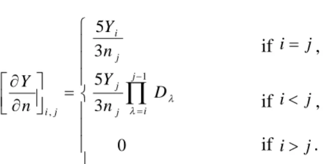
in Eq. (12) are expanded by the non-uniform flow equation. With the consideration of relative locations between the gauge station (i) and n-updating river segment (j), the elements of [ in Eq. (12) give three possible cases]m

                 



  0 3 5 3 5 1 , j i j j j i j i D n Y n Y n Y   if ij, if ij_, if ij. (17)

For the river system with tributaries, we assume that the n-updating in a tributary has no effect on the water depth of river segments in the main stream and other tributaries. The downstream n-updating in the main stream can affect the water depths in upper tributaries. Thus, the coefficient D is used to represent the backwater effects in the main stream as well as

tributaries.

2 ANALYSIS OF FLOOD FORECAST

As described in the previous section, the rationality and capability of the roughness updating technique in the dynamic routing model have been verified. Three typhoon events, Bilis (2000), Paripoo (2000), and Nari (2001), are then used to validate reliability of the roughness updating technique for stage forecasting. In the three typhoon events, the upstream and downstream boundary conditions are specified as the discharge and tidal stage, respectively. The input of the forecasting model includes the present time, observed and lead times forecasting data. The present time observed data are determined from the real time observed runoff at the five upstream boundaries and tidal stage at the river mouth. The six hour lead time forecast data at the upstream and downstream boundaries were obtained from the rainfall-runoff and tidal stage forecasting models, which were developed by Wang and Hsieh (2000) and Hsu et al. (2000). The model is run to perform the stage forecasting using roughness updating technique and the fixed Manning n for one to six hour ahead.

The stage profiles are used to examine the reliability of the initialization of stage profile for flood forecasting. The spatial variation of the maximum stage (t=15hr) along the Tanshui River-Tahan Creek is computed for the Xangsane typhoon event (shown in Figure 5). The figure shows that the stage profiles calculated with roughness updating technique is about the same as that calculated with real time stage correction (Hsu et al., 2003), and they agree better with the observed data than the values calculated with the fixed Manning n. The results illustrate that the dynamic routing model with roughness updating technique can provide the reliability of the initialization of stage profile that improves the accuracy of subsequent forecast.

Figure 12 exhibits the RMSE for one to six hours predictions. The RMSE values of stage increase with the forecasting lead time for the fixed Manning n. They are 0.588 m, 0.662 m, and 0.718 m for the one, three, and six hour lead-time predictions, respectively. The average RMSE is about 0.662 m. The results indicate that the fixed Manning n fails to respond to the resistance of river flow and provide inaccurate prediction. The RMSE of water stage calculated by the least-square method of stage correction (Hsu et al., 2003) were increased with lead time, such as, the one, three, and six hours ahead are 0.207 m, 0.405 m, and 0.676 m, respectively. The result shows that the improvement with real time stage correction method gradually diminished when one predicts far ahead in time. With the roughness updating in this study, the RMSE values for the one, three, and six hours lead time predictions are 0.201 m, 0.259 m, and 0.308 m, respectively. The average RMSE is about 0.262 m. The study found that the roughness updating

technique can promote a flood forecasting model in accuracy. The results indicate that the roughness updating technique can be an effective tool to minimize the error of the stage forecasting.

3 CONCLUSION

With the availability of the real time observed water depths at gauge stations in Tanshui River, the roughness updating technique of dynamic routing model has been presented using the Gauss-Newton method to minimize the error of the stage forecasting. Moreover, the Jacobian of the residuals is expanded by the Manning formula and the non-uniform flow equation to produce an automatic updating technique for the Manning roughness coefficient. The Xangsane typhoon event is selected to examine the initialization of stage profile, conservation of mass, iteration convergence, effectiveness evaluation, and convergence with different initial values by using the roughness updating technique. The results reveal that the dynamic routing model with roughness updating technique improves predictive capability.

Three typhoon events are used for the analysis of flood forecasting. The model is run to perform the stage forecasting using the roughness updating technique and the fixed Manning n for one to six hour lead time. The results demonstrate that the roughness updating technique is suitable for modeling the stages. However the model can improve the accuracy of stage hydrograph, stage profile, peak time, and satisfactory forecast stages from a lead time up to six hours. Therefore the new approach by combining the dynamic routing model with real time roughness updating technique can provide a useful tool for flood forecasting.

REFERENCES

Pizzuto, JJ.E. (1990), Numerical simulation of gravel river widening, Water Resources Research, 26(9), 1971-1980.

P.F. Randerson (1979), A simulation model of salt-marsh development and plant ecology, in Estuarine and Coastal Land Reclamation and Water Storage, edited by B. Knights and A.J. Phillips, pp. 48-67, Saxon House, Farnborough.

Steel, T.J., Pye, K. (1997), The development of salt marsh tidal creek networks: Evidence from the UK, in Proceedings of the Canadian Coastal Conference, pp. 267-280, CCSEA.

附錄 2

Minute of IAHR-APD ExCo Meeting in Venice, July, 2007

Time: July 3rd, 2007, 14:15-15:45

Place: room Sala Rossi Orago, Palazzo del Casino, Lido Island, Venice, Italy Attendants: Total 18 persons, they are:

J H W Lee, V Sundar, Hitoshi Tanaka, Bruce Melville, Gregory De Costa, Ming-Hsi Hsu, Lianxiang Wang, Babak Bozorgy, Chang Wan Kim, Etienne Mansard, Fulin Cai, Jianhua Wu, Xingnan Zhang, Mohamed S. Ghidaoui, Hyoseop Woo, Meg B Bishwakarwa, Guinevere Nalder, Janaka Wijiefunge

On the Occasion of the 32nd IAHR Congress in Venice, the IAHR-APD Executive Committee had a meeting to discuss a few things relating to APD affairs in the afternoon of July 3rd, 2007. The meeting lasted for about one and half hours. Prof. V Sundar, Chairman of APD ExCo, chaired the meeting that was attended by eighteen members. After self-introduction by the members present, a few issues were

addressed and discussed, which are listed below:

1. Reports were made by a few ExCo members on their activities after the 15thAPD Congress in India, relating to APD affairs. Prof. Melville expressed his desire to witness more IAHR activities in APD region. Prof.Tanakareported aworkshop “Vietnam- Japan Estuary Workshop”that was held in Vietnam during 22nd to 24th August, 2006 in which more than 150 scientists and engineers participated. Prof. Lianxiang Wang reported his participation at the IAHR-LAD Congress and ISHS symposium in Venezuela in October 2006 and also reported his discussion with the Hydraulic Structures section members on jointly holding 16thIAHR-APD congress and 3rdISHS symposium in China.

2. Prof. JHW Lee reported that, after three years of preparation, the quarterly Journal of

Hydro-Environment Research has been launched. The Launching Symposium was held in January 2007 in University of Hong Kong. The first issue would be printed in two weeks. Prof. Lee also said that the strategy of the IAHR Council meetings should be to attract more young scholars to join the organization. A suggestion is to have more student chapters. It was emphasized that ExCo members should try hard towards this. Field trip, for students could be another activity that could be looked into.

3. Dr. EPD. Mansard, the IAHR President, pleaded with members that efforts should be in by members

towards enrolling more members to IAHR. For the purpose to improve the financial position of IAHR it was suggested that it could be a policy to collect contribution of 3% of registration fee from the organizers of all IAHR-sponsored conferences.

4. Prof. Xingnan Zhang and his colleagues from Hohai University, reported the progress of the 16th IAHR-APD Congress and their preparations. The congress will be conducted jointly with 3rdInternational Symposium on Hydraulic Structures. A thorough discussion had been made on how to perform the two events in parallel and in cooperation. The first announcement will be distributed during the 32ndIAHR congress in Venice. In addition, Prof. Zhang introduced the details of getting to Nanjing, weather in Nanjing in October and the three proposed post-Congress tour lines, etc. Discussion was conducted on the date of the congress and proceedings. A few members expressed concerns that faculty members in the universities may not be able to attend the congress in October. A suggestion on proceedings was to have printed one as well as electronic one (CD Rom) similar to 15thIAHR-APD.

5. Decision on the venue of 17thIAHR-APD Congress was conducted. Two countries presented proposals for holding the 17thIAHR-APD Congress in 2010. Dr. B. Bozorgy from Iran read a letter, on behalf of Dr. Farhad Yazdandoost, to express their interest in holding the 17thIAHR-APD Congress, 2010 in Tehran, Iran.

Dr. De Costa and Dr. G Nalder from New Zealand submitted a report to hold the 17thIAHR-APD Congress, 2010 in Auckland, New Zealand. The Chairman opened a discussion. Some concerns on financial issue, potential participants and congress date etc. were put forward. After a deep discussion, a final decision has been made to conduct the 17thIAHR-APD Congress in New Zealand. An alternative date may be towards the end of November if concerning Spring Festival in February for many Asia countries. The First Announcement should be ready at the 17thIAHR-APD Congress in 2008.

6. Prof. V Sundar suggested having more workshops, seminars, ex. combined conference on tsunami

among Korea, Japan and Sri Lanka. He had informed about holding a Joint INDO-JAPAN workshop on Coastal protection in IIT Madras in India during 16thand 17thJuly that is sponsored by IAHR. For the next term of APD Executive Committee, there will be about 4 vacancies. Potential candidates may come from Malaysia, Sri Lanka, Thailand, Hong Kong and India, etc.

Attendants name list

IAHR-APD Executive Committee Meeting, in Venice, 2007-07-03

name country Email address ID

J H W Lee Hong Kong, China [email protected]; EC member

V Sundar India [email protected]; EC member

Hitoshi Tanaka Japan [email protected]; EC member

Bruce Melville New Zealand [email protected]; EC member

Gregory De Costa New Zealand [email protected]; EC member

Ming-Hsi Hsu Taiwan, China [email protected]; EC member

Lianxiang Wang China [email protected]; EC member

Babak Bozorgy Iran [email protected]; representative

Chang Wan Kim Korea [email protected]; representative

Etienne Mansard Canada [email protected]; IAHR Council

Fulin Cai China [email protected] invited

Jianhua Wu China [email protected]; invited

Xingnan Zhang China [email protected]; invited

Mohamed S. Ghidaoui Hong Kong, China [email protected]; invited

Hyoseop Woo Korea [email protected]; invited

Meg B Bishwakarwa Nepal [email protected]; invited

Guinevere Nalder New Zealand [email protected]; invited