國立臺灣大學工學院土木工程學系 博士論文
Department of Civil Engineering College of Engineering
National Taiwan University Doctoral Dissertation
應用支援向量機於颱風雨量及洪水預報
Typhoon Rainfall and Flood Forecasting Using Support Vector Machine
周揚敬
Chou, Yang-Ching
指導教授:林國峰 教授 Advisor: Lin, Gwo-Fong
中華民國 102 年 7 月
July, 2013
i
誌謝
首先誠摯的感謝指導教授林國峰老師悉心的指導,使我得以順利的完成博士 論文,老師對創新研究知識的追求以及嚴謹的做事態度,使我在這些年中獲益匪 淺。而論文初稿也承蒙老師與四位口試委員游保杉教授、陳主惠教授、陳明杰教 授、賴進松教授的指導,使內容更加完善,在此也至上十二萬分的謝意。
非常感謝谷榕學長帶我進入學術領域,陪著我克服許多困難,也讓我第一次 感受到文章被接受的喜悅。同樣非常感謝明璋學長幫研究室承擔了許多壓力,使 我可以更專注在學術研究上。珮瑜學姐的細心,亦讓我在論文撰寫上不會犯太多 錯。而在這漫長而苦悶的研究生涯中,感謝柏凱學長帶我們去光華散心,並帶領 我們進入快打領域。在準備畢業口試的過程中,更感謝學弟軒宇的大力幫忙。學 弟秉宸、明瑞、致瑋、信華、爵廷和學姊宜欣及學妹靚芸在研究上的協助,在此 亦致上由衷的感謝。
感謝所有家人的支持,以及恩威並施的爸媽。最後,要感謝一路陪伴,當我 最低潮時總是會鼓勵及支持我的老婆昭欣,因為有妳和寶貝兒女抖寶和菈菈,我 才可以堅持完成博士學位,非常感謝。
ii
中文摘要
本論文的主要目標為將支援向量機應用於洪災消減及災害預警上,主要可分為 以下兩個部分:
當颱風來襲時,雨量預報在大部分災害預警系統中皆扮演了非常關鍵的角色。
為了能更快速的得到準確的降雨預報,各個防災單位總是積極研發各種新式的預 報模式。本研究提出一種稱為支援向量機(support vector machine, SVM)的類神經網 路,並以此為基礎架構有效的颱風時雨量預報模式。相較於傳統上較常被使用的 倒傳遞類神經網路,基於統計學習理論的支援向量機具有三項優勢。第一、支援 向量機具備了更佳的學習能力(generalization ability),第二、支援向量機在架構和 權重的決定上保證有唯一解並且為全域最佳解,最後、支援向量機大量減少架構 模式所需的訓練時間。本研究以實際案例來說明支援向量機所具備的優勢。研究 結果顯示支援向量機相較於倒傳遞類神經網路不但能得到更加準確的預報結果,
並且有更佳的強健性,其中最大的優勢是能大幅的縮短架構模式所需的時間。除 了模式間的比較,為了能進一步提升長期預報的準確度,本研究更是新增了颱風 因子做為降雨預報模式的輸入項,並與沒加入颱風因子做為輸入項的模式進行比 較,以探討颱風因子對於雨量預報的影響。研究結果也證明了颱風因子可以有效 提升中長期預報的準確度。總結來說,本研究提出以支援向量機為基礎納入颱風 因子做為輸入項的預報模式確實能提升颱風時期雨量預報的準確度。而本模式亦
iii
預期能為洪水預報、土石流警戒等災害預警系提供幫助。
對於洪水預警來說準確的流量預報是非常重要的關鍵。因此在第二階段的研究 中提出一個以支援向量機為基礎,整合型的洪水預報模式來提升洪水預報的準確 度。整合型的洪水預報模式可以分為兩個部分,雨量預報單元及流量預報單元。
在第一階段,將以雨量及颱風因子作為輸入項發展雨量預報單元。接著將預報雨 量及觀測流量作為輸入項發展流量預報單元。為了驗證整合型洪水預報模式的能 力,本研究另外架構了直接納入觀測流量、雨量及颱風因子的洪水預報模式進行 比較。並以實際發生的颱風事件作為研究案例並預報未來 1 至 6 小時的流量。研 究結果顯示第一階段的雨量預報單元可以得到合理的預報結果。而將此預報雨量 納入輸入項的整合型洪水預報模式,相較於直接納入各因子的洪水預報模式能得 到更為準確的預報結果,甚至連尖峰流量亦有顯著的改善。值得注意的是,本研 究提出的模式更是顯著的提升了中長延時的預報準確度。歸納結果,本研究提出 的模式有效的減少了輸入項和輸出項間,隨著預報時間延長所帶來的負面影響,
因此才能在中長延時仍能維持一定的準確度。而此一優勢將對於提升颱風時期洪 水預警的反應時間有所幫助。
關鍵字:雨量預報,洪水預報,支援向量機,颱風因子,災害預警系統
iv
Abstract
The objective of this dissertation is to apply support vector machine for flood mitigation and disaster warning. There are two major parts in this paper, which are summarized in the following manner.
Typhoon rainfall forecasting plays a critical role in almost all kinds of disaster warning systems during typhoons. To obtain more effective forecasts of hourly typhoon rainfall, novel models with better ability are desired. Based on support vector machines (SVMs), which is a kind of neural networks (NNs), effective hourly typhoon rainfall forecasting models are constructed. As compared with back-propagation networks (BPNs) which are the most frequently used conventional NNs, SVMs have three advantages: (1) SVMs have better generalization ability; (2) the architectures and the weights of the SVMs are guaranteed to be unique and globally optimal; (3) SVM is trained much more rapidly. An application is conducted to clearly demonstrate these three advantages. The results indicate that the proposed SVM-based models are more well-performed, robust and efficient than the existing BPN-based models. To further improve the long lead-time forecasting, typhoon characteristics are added as key input to the proposed models. The comparison between SVM-based models with and without typhoon characteristics confirms the significant improvement in forecasting performance due to the addition of typhoon characteristics for long lead-time
v
forecasting. The proposed SVM-based models are recommended as an alternative to the existing models. The proposed modeling technique is also expected to be useful to support reservoir operation systems and flood, landslide, debris flow, and other disaster warning systems.
Accurate runoff forecasts are required to provide early warning of impending floods.
In this part, an integrated flood forecasting model based on the support vector machine (SVM) is proposed to improve the flood forecasting performance. In the first stage, the observed typhoon characteristics and rainfall are used to produce rainfall forecasts.
Then the forecasted rainfall and observed runoff are used to yield runoff forecasts. An actual application is performed to yield 1- to 6-h lead time runoff forecasts. The results show that the rainfall forecasting in the first stage can generate reliable rainfall forecasts, and the proposed model can provide accurate runoff forecasts, especially for the peak values. It is worth noting that the proposed model can significantly improve the 4- to 6-h lead time flood forecasting performance. In conclusion, the proposed model effectively mitigates the negative impact of increasing forecast lead time and is useful to improve the long lead time flood forecasting during periods of typhoon.
Keywords: rainfall forecasting, flood forecasting, support vector machines, typhoon characteristics, disaster warning systems.
vi
Contents
誌謝 ... i
中文摘要 ... ii
Abstract ... iv
Contents... vi
List of tables ... ix
List of figures ... x
Chapter 1 Introduction ... 1
1.1 Motivations ... 1
1.2 Backgrounds and Inspiration ... 3
1.2.1 Effective forecasting of hourly typhoon rainfall ... 3
1.2.2 Typhoon flood forecasting using integrated SVM ... 6
Chapter 2 Support vector machine ... 10
Chapter 3 Effective forecasting of hourly typhoon rainfall ... 15
3.1 Application ... 15
3.1.1 The Study Area and Data ... 15
3.1.2 Development of Models ... 17
3.1.3 Cross Validation and Performance Measures ... 19
3.2 Results and Discussion ... 21
vii
3.2.1 The Improvement Due to the Use of SVM-based Models Instead of BPN-based
Models ... 23
3.2.2 The Comparison of Robustness between SVM-based and BPN-based Models ... 28
3.2.3 The Comparison of Efficiency between SVM-based and BPN-based Models ... 32
3.2.4 The Improvement Due to the Addition of Typhoon Characteristics ... 33
3.3 Summary ... 40
Chapter 4 Typhoon flood forecasting using integrated SVM ... 42
4.1 Model development ... 42
4.1.1 Model construction ... 42
4.1.2 Performance measures ... 46
4.2 Application, results and discussion ... 48
4.2.1 Application ... 48
4.2.2 Results of rainfall forecasts ... 51
4.2.3 Influence of forecasted rainfall on flood forecasting ... 54
4.3 Summary ... 63
Chapter 5 Conclusions ... 65
5.1 Effective forecasting of hourly typhoon rainfall ... 65
5.2 Typhoon flood forecasting using integrated SVM ... 66
References ... 69
viii
Publications ... 74
ix
List of tables
Table 3.1 Descriptions of typhoon events used in the modeling ... 16
Table 3.2 Coefficient of efficiency (CE), mean absolute error (MAE) and root mean square error (RMSE) for various models ... 22
Table 3.3 Paired comparison t-tests of three performance measures (CE, MAE and RMSE) resulting from SVM-RT and BPN-RT and from SVM-RT and SVM-R ... 22
Table 4.1 Description of typhoon events used in the modeling ... 50
Table 4.2 Input variables to the NN models ... 52
Table 4.3 MCE and MEPR for various models ... 54
Table 4.4 Paired comparison t-tests of two performance measures (CE and EPR) resulting from SVM-QRT and SVM-QRf. ... 60
x
List of figures
Figure 2.1 Architectural graph of SVM ... 14
Figure 3.1 The study area ... 16
Figure 3.2 Flowcharts of (a) the model development and (b) the lag length determination ... 18
Figure 3.3 (a) CE values of SVM-RT and BPN-RT and (b) the improvement in CE due to the
use of SVM-based models instead of BPN-based models ... 25
Figure 3.4 (a) MAE, (b) RMSE values of SVM-RT and BPN-RT, and (c) the percentages of
decrease in MAE and RMSE due to the use of SVM-based models instead of BPN-based
models ... 27
Figure 3.5 (a) CV values for each typhoon event resulting from BPN-RT trained with 30
different sets of initial weights. (b) RMSE values of BPN-RT trained with 30 different sets of
initial weights and the constant CE value of SVM-RT (taking Typhoon Gladys as an example) ..
... 31
Figure 3.6 (a) CE values of SVM-RT and SVM-R and (b) the improvement in CE due to the
addition of typhoon characteristics ... 35
Figure 3.7 (a) MAE, (b) RMSE values of SVM-RT and SVM-R, and (c) the percentages of
decrease in MAE and RMSE due to the addition of typhoon characteristics ... 37
xi
Figure 3.8 The number of events for which the model with each single typhoon characteristic
yields a higher CE value than SVM-R ... 39
Figure 4.1 Architectural graphs of (a) the proposed model and (b) the existing model ... 43
Figure 4.2 Flowchart of the model development ... 45
Figure 4.3 The study area and locations of rainfall and water-level stations ... 49
Figure 4.4 MCE values of SVM-QRT, BPN-QRT and SVM-QRi ... 53
Figure 4.5 RMSE values of the rainfall forecasts ... 53
Figure 4.6 (a) MCE values of SVM-QRT and SVM-QRf and (b) the improvement in MCE due to the use of SVM-QRf instead of SVM-QRT ... 57
Figure 4.7 (a) MEPR values of SVM-QRT and SVM-QRf and (b) the improvement in MEPR due to the use of SVM-QRf instead of SVM-QRT ... 58
Figure 4.8 Number of events for which (a) CE values of SVM-QRf are higher than those of SVM-QRT and (b) EPR values of SVM-QRf are lower than those of SVM-QRT ... 60
Figure 4.9 Comparison of the observed runoff with the 1-h lead time forecasts resulting from (a) SVM-QRf and (b) SVM-QRT for Typhoon Haitang ... 61
Figure 4.10 Comparison of the observed runoff with the 1- to 6-h lead time forecasts resulting from SVM-QRf ... 62
1
Chapter 1 Introduction
1.1 Motivations
The island of Taiwan is situated in one of the main paths of the north-western Pacific typhoons. Each year, three to four typhoons attack the island on average. The torrential rain brought by typhoons (tropical cyclones occurring in the western Pacific Ocean) frequently lead to serious disasters, such as flooding, landslide or debris flow.
To mitigate disasters due to typhoons, the development of flood warning systems are always needed. However, the highly non-linear and complex processes of typhoon rainfall and runoff make it difficult to construct a reliable physically-based model. To obtain more effective forecasts of typhoon rainfall and runoff, the development of better models has always been regarded as an important task.
An attractive alternative to the physically-based models is neural networks (NNs), which is a kind of information processing system with great flexibility in modeling nonlinear processes. The conception of NNs was inspired by a desire to understand human brain. Comprehensive reviews of the applications of NNs in hydrology have been presented by ASCE Task Committee (2000a, 2000b) and Maier and Dandy (2000).
More recently, hydrologists, water resources engineers and managers have inspected more various applications of NNs for hydrologic forecasting, such as streamflow
2
forecasting (e.g., Tingsanchali and Gautam, 2000; Lin and Chen, 2004; Toth and Brath, 2007), tidal level forecasting (e.g., Supharatid, 2003), and groundwater level forecasting (e.g., Lin and Chen, 2005a). In addition to the great flexibility in modeling nonlinear systems, NNs are very suitable for being integrated with decision- support systems due to their high computational efficiency. For instance, NN-based models have been integrated with reservoir operation systems (e.g., Khalil et al., 2005; Chaves and Kojiri, 2007; Tu et al., 2008), city flood control systems (Chang et al., 2008), as well as debris flow warning systems (Chang et al., 2007).
Because of their flexibility in modeling nonlinear systems and their computational efficiency, NNs have gained a considerable attention. More recently, a powerful kind of NNs named Support Vector Machines (SVMs) have attracted the attention of some hydrologists but only limited application are examined, such as hydrologic time series analysis (Liong and Sivapragasam, 2002; Yu et al., 2004; Asefa et al., 2005;
Sivapragasam and Liong, 2005; Yu and Liong, 2007), reservoir inflow forecasting (Lin and Chen, 2009a), and streamflow forecasting (Yu et al., 2006; Kalra and Ahmad, 2009).
Based on statistical learning theory, SVMs have advantages over back-propagation networks (BPNs) which are the most frequently used conventional NNs. Firstly, SVMs have better generalization ability to relate the relatively irrelative input to the desired output. This advantage is very helpful to decrease the negative impact when
3
increasing forecast lead-time. In other words, SVMs are capable of producing acceptably accurate forecasts for longer lead-time. Secondly, the optimization algorithm for SVMs is more robust, and the architectures and the weights of the SVMs are guaranteed to be unique and globally optimal. The performance of SVM-based models is more reliable because of the robust optimization algorithm. Finally, SVMs are trained much more rapidly. Thus, SVM-based models are more suitable to be integrated with disaster warning systems and decision support systems.
Due to the aforementioned attractive advantages, SVMs have emerged as an alternative data-driven tool in many conventional NN dominated fields. In this dissertation, SVMs were introduced and applied to typhoon rainfall and flood forecasting.
1.2 Backgrounds and Inspiration
1.2.1 Effective forecasting of hourly typhoon rainfall
Rainfall forecasting plays a critical role in almost all kinds of disaster warning systems during typhoons. In the Taiwan area, typhoon rainfall often causes casualties and has major economic impacts; however, it is an important water resource. As a typhoon approaches the island, the major goal of reservoir operation is to control floods.
But when the typhoon leaves, the goal switches to restore sufficient water for future
4
usage. To achieve these two goals, reservoir operation should be appropriately conducted. More effective (or more accurate and reliable) forecasts of hourly rainfall are required as a vital reference for hourly reservoir inflow forecasting and for making important reservoir operation decisions. In addition, an improved hourly rainfall forecasting is expected to be useful to support flood, landslide, debris flow and other disaster warning systems.
As to rainfall forecasting, applications of NNs have also been presented (e.g., Luk et al., 2001; Chiang et al., 2007), but studies on NN-based models for hourly typhoon rainfall forecasting are still limited. To provide effective forecasts of hourly typhoon rainfall for being integrated with decision support systems, Lin and Chen (2005b) have assessed the potential of BPNs. The results indicated that BPN-based models yield acceptable forecasts for a lead time of one to two hours only. To provide effective warnings, longer lead-time forecasting is needed. However, as the forecast lead-time increases, the correlation between desired output and available input decreases. The data used for long lead-time forecasting include more relatively irrelative information which seriously undermines the performance of BPN-based models. Based on previous studies (Lin and Chen, 2005b, 2008), the generalization ability of BPNs was not good enough. To obtain effective forecasts of hourly rainfall for longer lead-time forecasting, it is justified to propose novel models with better generalization ability.
5
In this study, SVMs were used to construct typhoon rainfall forecasting models.
Hong and Pai (2007) have constructed a SVM-based typhoon rainfall forecasting model with only antecedent rainfall as input. Their forecasts were acceptably accurate but only for one-hour ahead forecasting. With only antecedent rainfall as input, the performance of models usually decreases rapidly with increasing forecast lead-time.
To further enhance the long lead-time forecasting, typhoon characteristics were regarded as key input and added to the proposed SVM-based models. Lin and Chen (2005b) have confirmed that the trend of rainfall could be demonstrated by typhoon characteristics when a typhoon was nearby. It is reasonable to speculate that typhoon characteristics are capable of providing valuable information for longer lead-time forecasting. Such a speculation has prompted an investigation into the influence of typhoon characteristics on rainfall forecasting, in particular, for long lead-time forecasting.
The objective of this study was to provide effective forecasts of hourly rainfall for supporting reservoir operation systems during typhoons. For this purpose, SVM-based, instead of BPN-based models with typhoon characteristics were proposed to yield 1-to 6-h lead time forecasts. In order to compare SVMs and BPNs, BPN-based models with same input are also constructed. Moreover, to assess the improvement in forecasting performances due to the addition of typhoon characteristics, two types of
6
model input (with and without typhoon characteristics) are designed for SVM-based models. Finally, an application was conducted and 11 typhoon events were used in this study. To reach just conclusions, cross validations were applied to evaluate the overall performance of the models and the statistical significance of the improvement in forecasting performance was identified by paired comparison t-tests. The results demonstrated the superiority of the proposed models more clearly.
1.2.2 Typhoon flood forecasting using integrated SVM
To mitigate disasters caused by typhoons, accurate and reliable flood forecasts are essential to provide early warning of impending floods and their improvement has been verified as a crucial task. In recent years, NNs have been successfully employed in various hydrologic modeling applications (e.g., de Vos and Rientjes, 2005; Hu et al., 2007; Lin and Chen, 2004; Wu and Chau, 2011) and specifically for rainfall and flood forecasting (e.g., Chang et al., 2004; Chiang et al., 2007; Lin and Chen, 2005b; Lin et al., 2010; Luk et al., 2001; Pramanik et al., 2011; Rathinasamy and Khosa, 2012; Toth and Brath, 2007). The major advantage of NNs is their capability to simulate complex relationship between desired output and available input given the existence of sufficient training datasets.
However, flood forecasting performance of most NNs decreases rapidly with
7
increasing of the forecast lead time. Operational agencies which are responsible for flood mitigation and warnings could well benefit from improved forecast accuracy of the longer lead times. Multi-stage NN-based models were developed in attempt to achieve a longer as well as accurate forecast lead time (Chang et al., 2007; Lin and Wu, 2011). The concept of multi-stage NN-based models is that two or more NN-based models are connected. Using the two-stage as an example, the connection between the two stages is that forecasted values from the first-stage module are used as input to the second-stage module. It is widely known that rainfall is one of the most important inputs to flood forecasting model and the accuracy of long lead time flood forecasting can be advanced with more accurate rainfall forecasts. Lin et al. (2009c) improved longer lead time streamflow forecast by adopting BPNs to predict rainfall as input to a Radial Basis Function (RBF)-based reservoir inflow forecasting model. Chiang and Chang (2009) used Quantitative Precipitation Forecasting (QPF) information as input to Recurrent Neural Network (RNN)-based flood forecasting model and reported a similar finding, that is, the forecasted rainfall was capable of providing useful information for flood forecasting, especially for long lead time.
In previous studies, multi-stage NN-based flood forecasting models were based on conventional NNs. The architecture and the weights of these conventional NNs were determined by a trial and error procedure which consisted of iterative time-consuming
8
process. Although the selection of NN-based models generally disregard the efficiency of the model training, it is essential to develop a well-performing model that can be quickly trained.
In this study, an integrated support vector machine (SVM)-based model was developed to yield 1- to 6-h lead time runoff forecasts. SVMs have been used for hydrologic time series forecasting (Liong and Sivapragasam, 2002; Sivapragasam and Liong, 2005; Wu et al., 2009; Yu and Liong, 2007; Yu et al., 2004). More recently, Rasouli et al. (2012) employed SVM and other machine learning methods with weather and climate inputs to forecast daily streamflow. According to statistical learning theory, SVM has better generalization ability and requires less training time than conventional NNs (e.g., BPN). For both rainfall and inflow forecasting, Lin et al.
(2009a, 2009b) demonstrated that SVM-based models outperform BPN-based models.
Moreover, the development of SVM-based models is efficient and thus expected to be suitable for development of the integrated model presented herein.
The objective of this study is to demonstrate an integrated SVM-based model for typhoon flood forecasting. A rainfall forecasting module was established in the first stage to pre-process the typhoon information (namely, typhoon characteristics and rainfall) as well as to produce rainfall forecasts. Afterwards, the rainfall forecasts
9
along with the observed runoff were used as input to the flood forecasting module in the second stage. This procedure was expected to reduce the input dimensionality and improve the performance of the longer forecast lead times, especially for the prediction of peak runoff.
10
Chapter 2 Support vector machine
In the early 1990s, Vapnik developed SVMs for classification and then extended for regression (Vapnik, 1995). There are two major differences between the SVMs and the BPNs. Firstly, instead of empirical risk minimization (ERM), the structural risk minimization (SRM) induction principle is used to construct SVMs. For training BPNs, the only one objective is to minimize the total error (or empirical risk). As to SVMs, according to the SRM induction principle, both the empirical risk and the model complexity should be minimized simultaneously. The use of SRM induction principle results in the better generalization ability of SVMs. Another major difference is the determination of the model architecture and the weights. For BPNs, the architecture and the weights are respectively determined by a trial-and-error procedure and an iterative process (the error back-propagation algorithm), which both are very time-consuming. Vapnik (1995) dispensed with the time-consuming training process and expressed the determination of the architecture and weights of SVMs in terms of a quadratic optimization problem which can be rapidly solved by a standard programming algorithm. In this section, the methodology of the support vector regression (SVR) used in this paper is briefly described and more mathematical details about SVR can be found in several text books (Vapnik, 1995; Vapnik, 1998; Cristianini and Shaw-Taylor, 2000).
11
Based on N training datad [( 1, 1),( 2, 2),...,( , )]
d
d N
N y
y
y x x
x , the objective of the
support vector regression is to find a non-linear regression function to yield the output yˆ, which is the best approximate of the desired output y with an error tolerance of . Firstly, the input vector x is mapped onto a higher dimensional feature space by a non-linear function(x). Then the regression function that relates the input vector x to the output yˆ can be written as
b f
yˆ (x)wT(x) (2.1)
where w and b are weights and bias of the regression function, respectively. Based on the SRM induction principle, w and b are estimated by minimizing the following structural risk function:
Nd
i
i
T C L y
R
1
ˆ) 2 (
1 w
w (2.2)
where the Vapnik’s -insensitive loss function L is defined as
y y y y
y y y
y y
L ˆ for ˆ
ˆ for
| 0
| ˆ ˆ)
( (2.3)
The first and second terms in Eq. (2) represent the model complexity and the empirical error, respectively. The trade-off between the model complexity and the empirical error is specified by a user-defined parameter C and C 1 is set herein.
Vapnik (1995) expressed the SVR problem in terms of the following optimization
12
problem:
l i
y b y
y
b y
y y
C b
R
i i
i i
i T i i
i i
T i i i
N
i
i i
T d
,..., 2 , 1
0
0
) ) ( ˆ (
) ) ( ˆ (
subject to
) 2 (
) 1 , , , (
Minimize
1
x w
x w
w ξ w
ξ w
(2.4)
where and , which are slack variables, represent the upper and the lower training errors, respectively. The above optimization problem is usually solved in its dual form using Lagrange multipliers. Rewriting Eq. (4) in its dual form and differentiating with respect to the primal variables (w,b,ξ,ξ) gives
d i i N
i
i i
N
i
j N
j
i j j i i N
i
i i N
i
i i i
N i
C C y
d
d d
d d
,..., 2 , 1
0
0
0 ) (
subject to
) ( ) ( ) )(
2 ( ) 1 (
) (
Maximize
1
1 1
T 1
1
x x
(2.5)
where and are the dual Lagrange multipliers. Note that the solution to the optimal problem (Eq. (5)) is guaranteed to be unique and globally optimal because the objective function is a convex function.
13
The optimal Lagrange multipliers * are solved by the standard quadratic programming algorithm and then the regression function can be rewritten as
Nd
i
i
iK b
x f
1
* ( , )
)
( x x (2.6)
where the kernel function K(xi,x) is defined as
) ( ) ( ) ,
(xi x xi T x
K (2.7)
The kernel function used in this paper is the radial basis function:
)
| 1 |
exp(
) ,
(x x xix 2
x
i n
K (2.8)
where n is the number of components in input vector x x.
Some of solved Lagrange multipliers () are zero and should be eliminated form the regression function. Finally, the regression function involves the nonzero Lagrange multipliers and the corresponding input vectors of the training data, which are called the support vectors. The final regression function can be rewritten as
sv
1
) , ( )
(
N
k
k
kK b
f x x x (2.9)
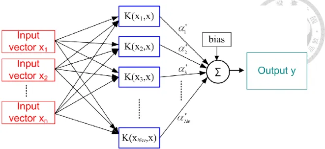
where x denotes the k kth support vector and N is the number of support vectors. sv The architecture of a SVM is presented in Fig. 2.1.
14
Figure 2.1 Architectural graph of SVM
15
Chapter 3 Effective forecasting of hourly typhoon rainfall
3.1 Application
3.1.1 The Study Area and Data
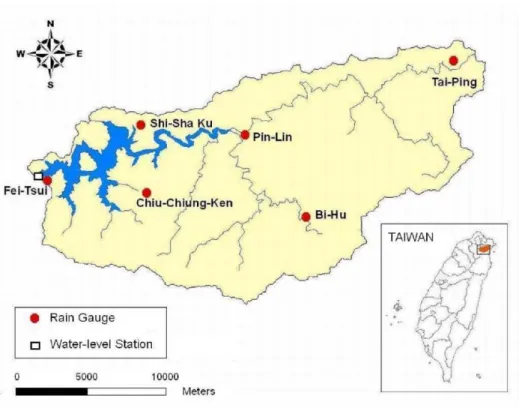
The study area is the Fei-Tsui Reservoir Watershed in northern Taiwan. The Fei-Tsui Reservoir is located downstream of three major tributaries (the Kingkwa Creek, the Diyu Creek and the Peishih Creek). The reservoir has a surface area of 10 km2, a mean depth of 40 m, a maximum depth of 120 m, a full capacity of 406 million m3, and a total watershed area of 303 km2. From 1988 to 2007, the maximum and average yearly rainfall is 5736.6 mm and 3808.6 mm, respectively. Fig. 3.1 shows the study area and the locations of six rain gauges (Fei-Tsui, Pin-Lin, Shi-San-Ku, Chiu-Chiung-Ken, Bi-Hu and Tai-Pin). The rainfall data are obtained from the Water Resources Agency and the typhoon characteristics are collected from the Central Weather Bureau. The time periods of the data of rainfall and typhoon characteristics are hourly. A total of 11 typhoon events with typhoon characteristics and rainfall data available simultaneously are used herein. Table 3.1 summarizes the date of occurrence and duration of these 11 typhoon events. The typhoon characteristics include the position of the typhoon center, the distance between the center and the reservoir, the maximum wind speed near the center, the atmospheric pressure of the center, the radius of winds over 15 m/s, and the speed of the typhoon movement.
16
Table 3.1 Descriptions of typhoon events used in the modeling Name of typhoon Date Duration
(hour)
Maximum wind speed (m/s)
Maximum hourly rainfall (mm)
Ted 1992/09/20 69 108 19.6
Tim 1994/07/09 49 191 16.3
Gladys 1994/08/31 32 126 31.0
Seth 1994/10/08 75 184 18.7
Herb 1996/07/30 70 191 46.7
Haiyan 2001/10/15 28 130 14.1
Rammasun 2002/07/03 32 165 22.5
Nock-Ten 2004/10/24 44 155 35.4
Haitang 2005/07/17 66 198 42.5
Matsa 2005/08/04 48 144 31.2
Talim 2005/08/31 43 191 42.6
Figure 3.1 The study area
17
3.1.2 Development of Models
In this study, SVM-based models with typhoon characteristics (SVM-RT) are proposed to yield 1- to 6-h lead time rainfall forecasts. To make comparisons between SVMs and BPNs, BPN-based models with typhoon characteristics (BPN-RT) are constructed. Otherwise, SVM-based models without typhoon characteristics (SVM-R) are also constructed to evaluate the improvement in forecasting performance due to the addition of typhoon characteristics. Hence, a total of 18 NN-based forecasting models (SVM-RT, BPN-RT and SVM-R for 1- to 6-h lead time forecasts) are constructed.
The SVM-R has a general form as
, 1, , ( 1)
LR
t t
t t
t f R R R
R (3.1)
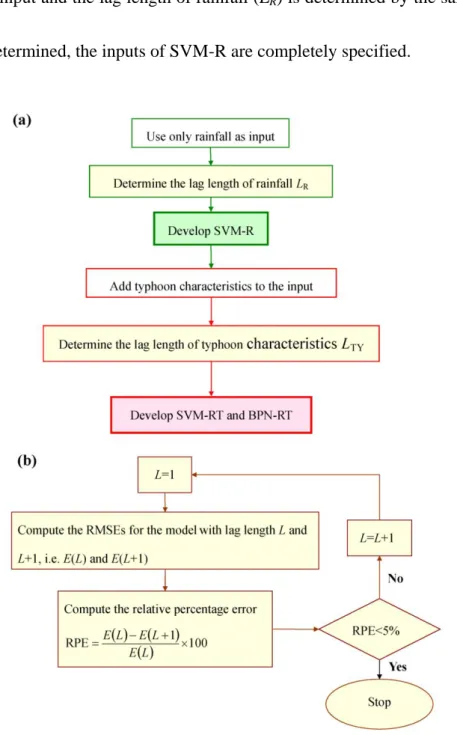
where t is the current time, t is the lead-time period (from one to six hours), R t is rainfall at time t , and LR denotes the lag length of rainfall. The model development is schematized in Fig. 3.2(a). Firstly, only rainfall is used as input and the lag length of rainfall (LR) is determined by the process shown in Fig. 3.2(b). The
criterion for selecting the lag lengths is the relative percentage error (RPE):
1 100RPE
L E
L E L
E (3.2)
where E
L and E
L1
are the RMSEs for models with L and L1 lag18
lengths, respectively. In general, the RMSE decreases with increasing lag term.
When the RPE is less than 5%, the increase of lag lengths is stopped. Then rainfall is added to the input and the lag length of rainfall (LR) is determined by the same process.
Once LR is determined, the inputs of SVM-R are completely specified.
Figure 3.2 Flowcharts of (a) the model development and (b) the lag length determination
19
Based on the SVM-R, all typhoon characteristics (include the position of the typhoon center, the distance between the center and the reservoir, the maximum wind speed near the center, the atmospheric pressure of the center, the radius of winds over 15 m/s, and the speed of the typhoon movement) are then added to develop the SVM-RT and
BPN-RT. The form of the SVM-RT and BPN-RT is
, 1, , ( 1), , 1, , ( 1)
TY
R t t t L
L t t
t t
t f R R R TY TY TY
R (3.3)
where TY is typhoon characteristics at time t, and t LTY denotes the lag length of typhoon characteristics which is determined by the same process shown in Figure 3.2(b).
To further investigate the influence of each typhoon characteristic on rainfall forecasting, a total of six models with single typhoon characteristic are constructed by individually adding each typhoon characteristic in turn to the model without typhoon characteristics (SVM-R).
3.1.3 Cross Validation and Performance Measures
For event-based data, the collected events are usually separated into two sets of data:
training and testing. Some events are chosen as training data and used to construct NN-based models. Then the performance of the NN-based models is tested by the remaining events which are not used in the training process. Different selections of training data and testing data produced different results and sometimes lead to different
20
conclusions. To reach just conclusions, cross validations are conducted herein. Each single typhoon event (except Typhoon Herb) is used to test the NN-based models in turn.
Typhoon Herb yielded the maximum rainfall and should be used as training data.
Then conclusions are drawn based on the overall performance for the 10 testing events.
Three performance measures are used to evaluate the model performance herein.
1. Coefficient of efficiency (CE):
n
t t n
t
t t
R R
R R
1
2 1
2
) (
ˆ ) ( 1
CE (3.4)
where R and t Rˆ denote the observed and forecasted rainfall at time t , respectively, t R is the average of the observed rainfall, and n is the number of forecasts. If the CE value is equal to one, the forecasts are perfect.
2. Mean absolute error (MAE):
n
t
t
t R
n 1 R 1 ˆ
MAE (3.5)
3. Root mean square error (RMSE):
n
t
t
t R
n 1 R
ˆ 2
RMSE 1 (3.6)
21
3.2 Results and Discussion
Table 3.2 presents the three performance measures (CE, MAE and RMSE) of three NN-based models (SVM-RT, BPN-RT and SVM-R) for 1- to 6-h lead time rainfall forecasts. According to the three performance measures, the proposed SVM-based model with typhoon characteristics (SVM-RT) produces the best performance and BPN-RT performs the worst among all models. To further identify whether SVM-RT performs significantly better than BPN-RT and SVM-R for the same testing event, paired comparison t -tests are conducted at the 1% significance level. The equation of
t -tests is defined as
n s X S
t X
X
0
0
(3.7)
The results listed in Table 3.3 show that SVM-RT significantly yields higher CE, lower RMSE, and lower MAE values than both BPN-RT and SVM-R. To clearly demonstrate the superiority of the proposed models (SVM-RT), more performance comparisons are discussed in depth in the rest of this section.
22
Table 3.2 Coefficient of efficiency (CE), mean absolute error (MAE) and root mean square error (RMSE) for various models
Lead time (hour)
CE
SVM-RT BPN-RT SVM-R
1 0.44 0.35 0.43
2 0.32 0.17 0.26
3 0.24 0.04 0.17
4 0.24 0.02 0.10
5 0.21 -0.12 0.01
6 0.21 -0.19 -0.02
Lead time (hour)
MAE (mm)
SVM-RT BPN-RT SVM-R
1 3.21 3.85 3.29
2 3.59 4.34 3.77
3 3.91 4.67 4.12
4 3.93 4.82 4.31
5 4.04 5.08 4.58
6 4.20 5.32 4.75
Lead time (hour)
RMSE (mm)
SVM-RT BPN-RT SVM-R
1 5.14 5.54 5.21
2 5.69 6.27 5.95
3 6.04 6.81 6.30
4 6.06 6.88 6.62
5 6.23 7.40 6.96
6 6.28 7.69 7.11
Table 3.3 Paired comparison t-tests of three performance measures (CE, MAE and RMSE) resulting from SVM-RT and BPN-RT and from SVM-RT and SVM-R
Model Alternate
hypothesis
t-statistic Statistically significant at the 1% level
SVM-RT CESVM-RT>CEBPN-RT 3.18 Yes
and MAESVM-RT<MAEBPN-RT 4.35 Yes
BPN-RT RMSESVM-RT<RMSEBPN-RT 3.37 Yes
SVM-RT CESVM-RT>CESVM-R 6.47 Yes
and MAESVM-RT<MAESVM-R 7.20 Yes
SVM-R RMSESVM-RT<RMSESVM-R 6.85 Yes
Note: The critical t-value is 2.39.
23
3.2.1 The Improvement Due to the Use of SVM-based Models Instead of BPN-based Models
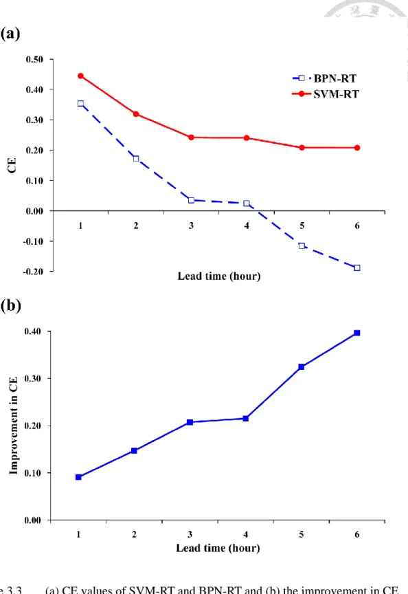
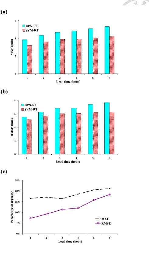
To highlight the improvement in forecasting performance due to the use of SVM-based models instead of BPN-based models, we first focus on the comparison between the proposed SVM-based models (SVM-RT) and BPN-based models with the same input (BPN-RT). As shown in Fig. 3.3(a), the CE values of both SVM-RT and BPN-RT decrease with increasing forecast lead-time. However, it is clear that SVM-RT yields significantly higher CE values than BPN-RT for 1- to 6-h lead-time forecasting. Thus, it is concluded that SVM-based models perform better than BPN-based models. Fig. 3.3(a) also shows that the CE values of SVM-RT decrease more slowly than those of BPN-RT. For 1- to 2-h lead time forecasts, the CE values of SVM-RT only decrease from 0.44 to 0.32, but those of BPN-RT rapidly decrease from 0.35 to 0.17. Then, for 3- to 6-h lead time forecasts, the performance of BPN-RT gets worse and the CE values are almost equal or even lower than zero. It is clear that BPN-RT cannot yield effective forecasts when the forecast lead-time is greater than two hours. As to SVM-RT, the performance is still acceptable for long lead-time forecasting. For 3- to 6-h lead time forecasts, the CE values only decrease from 0.24 to 0.21. The use of SVM-based models instead of BPN-based models effectively decreases the negative impact of increasing forecast lead-time.
24
The improvement in CE due to the use of SVM-based models instead of BPN-based models presented in Fig. 3.3(b) more clearly shows that the proposed SVM-based models (SVM-RT) effectively improve the forecasting performance. For 1- to 6-h lead time forecasts, the improvement in CE increases from 9% to 40%. It is clear that SVM-based models are more appropriate for long lead-time forecasting than BPN-based models. There are reasonable explanations for the results presented in Fig.
3.3. As the forecast lead time increases, the correlation between desired output and available input decreases. Hence the data used for long lead-time forecasting include more relatively irrelative information and the models require better generalization ability to relate the input to the desired output. Based on the statistical learning theory, SVMs have better generalization ability than BPNs. Thus, a greater improvement in performance could be obtained by using SVM-based models instead of BPN-based models, especially for long lead-time forecasting.
25
Figure 3.3 (a) CE values of SVM-RT and BPN-RT and (b) the improvement in CE due to the use of SVM-based models instead of BPN-based models
26
According to other two performance measures (MAE and RMSE), similar results are also obtained. For 1- to 6-h lead time forecasts, the bar charts presented in Fig. 3.4(a) and 3.4(b) clearly show that both MAE and RMSE values of SVM-RT are lower than those of BPN-RT. In addition, the MAE and RMSE values of SVM-RT increase more slowly than those of BPN-RT with increasing forecast lead-time. The negative impact of increasing forecast lead-time has been effectively decreased by using SVM-based models instead of BPN-based models. The percentages of decrease in MAE and RMSE due to the use of SVM-based models instead of BPN-based models are presented in Fig. 3.4(c). For 1- to 6-h lead time forecasts, SVM-RT respectively decreases MAE and RMSE values from 17% to 21% and from 7% to 18% as compared to BPN-RT.
Again, the results confirm that the proposed SVM-based models (SVM-RT) effectively improve the forecasting performance.
27
Figure 3.4 (a) MAE, (b) RMSE values of SVM-RT and BPN-RT, and (c) the percentages of decrease in MAE and RMSE due to the use of SVM-based models
instead of BPN-based models
28
3.2.2 The Comparison of Robustness between SVM-based and BPN-based Models
A robust parameter optimization algorithm is required to construct a robust model which can yield reliable forecasts. But for hydrological models, there are very limited studies on the related topics. In addition to better generalization ability, the robustness of optimization algorithm for SVMs is one of the major advantages over BPNs. For a robust optimization algorithm, the obtained optimal weights are slightly influenced by the initial conditions, such as initial weights. On the contrary, the optimization algorithm is less robust, if obtained optimal weights highly depend on the initial weights.
For BPNs, the weights are determined by an iterative process and the optimal weights depend on the initial weights which are usually set randomly. Even when a BPN is trained with the same training data, but different initial weights may lead to different optimal weights and, of course, different forecasting performance. Hence, enough sets of initial weights should be tried to get the globally optimal weights. Based on our experiences, at least 30 sets of initial weights are required to obtain a reliable forecasting performance. As to SVMs, the determination of the architecture and the weights is expressed in terms of a quadratic optimization problem with a convex objective function, and the weights are solved by the standard programming algorithm.
The solved weights are guaranteed to be unique and globally optimal. Thus, the same
29
optimal weights could be always obtained when a SVM is trained with the same training data. Theoretically, the performance of SVM-based models is more reliable than that of BPN-based models
To demonstrate the robustness of SVM-based models more clearly, SVM-RT and BPN-RT are taken for example herein. Being trained with 10 typhoon events and tested by the remaining one event, SVM-RT yields a constant RMSE. As to BPN-RT, different initial weights lead to different RMSE values even when the same training and testing data are used. In this case, BPN-RT is trained with 30 different sets of initial weights and hence yields 30 different RMSE values for each testing typhoon event.
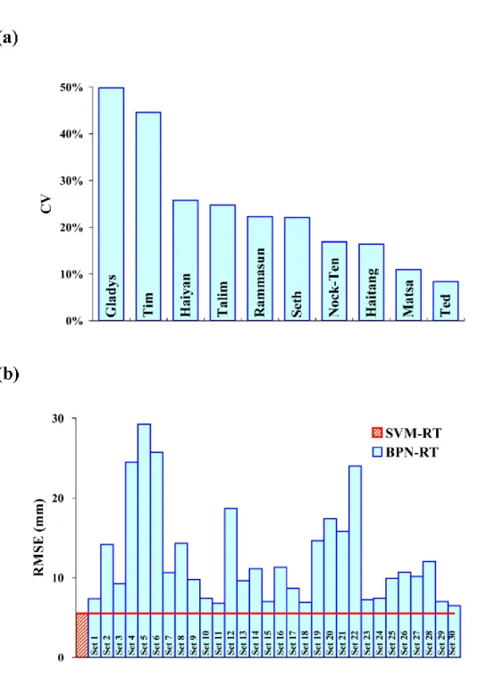
The lack of robustness can be observed by the variation in RMSE, which is evaluated by the coefficient of variation (CV). A higher CV value of RMSE represents the higher variation in RMSE and also indicates that the performance of BPN-RT is less reliable. For each typhoon event, the CV is calculated from a data set of 30 RMSE values resulting from BPN-RT trained with 30 different sets of initial weights. Fig.
3.5(a) presents the CV values of 10 typhoon events. Among 10 events, 6 events have CV values greater than 20% and 2 events exceeding 40%. For Typhoon Gladys, BPN-RT yields the highest CV value of 50%. The result clearly shows that BPN-RT lacks robustness.
30
To discuss the robustness of SVM-RT and BPN-RT in depth, the performance of SVM-RT and BPN-RT tested by Typhoon Gladys is highlighted. Fig. 3.5(b) presents the RMSE values of BPN-RT trained with 30 different sets of initial weights and the constant RMSE value of SVM-RT. As shown in Fig. 3.5(b), the constant RMSE yielded by SVM-RT indicates that SVM-RT is a robust model and the performance is reliable. On the contrary, it is found that the variation in RMSE for BPN-RT is very significant. The great variation in RMSE confirms that the initial weights have great influence on the forecasting performance of BPN-based models. Thus, enough sets of initial weights should be tried to ensure the satisfactory and reliable results. For the case of Typhoon Gladys, 16 sets (more that 50% of all sets) have significantly worse performances (with RMSE>10 mm). It is reasonable to speculate that the iterative processes have been trapped in the local optimal solutions and such a situation can be completely avoided by the use of SVMs. Based on the above results, it is concluded that SVM-based models are more robust than BPN-based models.
31
Figure 3.5 (a) CV values for each typhoon event resulting from BPN-RT trained with 30 different sets of initial weights. (b) RMSE values of BPN-RT trained with 30 different sets of initial weights and the constant CE value of SVM-RT (taking Typhoon
Gladys as an example)
32
3.2.3 The Comparison of Efficiency between SVM-based and BPN-based Models
Efficiency is an important issue for models, but the efficiency of hydrological models is only assessed in limited studies. Lin and Chen (2005c, 2006) have examined the efficiency of BPN-based models and the results clearly show the time-consuming training process of BPNs. In many conventional NN dominated fields, SVMs defeat BPNs because of much higher efficiency. However, the high efficiency of SVMs has also received little attention in the hydrologic domain. According to the previous study (Lin and Chen, 2009), SVMs are trained much more rapidly than BPNs. In fact, the optimal architecture and weights of SVMs are rapidly “solved”, not “searched”.
On the contrary, BPNs are trained by the error back-propagation algorithm which is a very time-consuming iterative process. Based on the methodologies of SVMs and BPNs, it is obvious that the development of SVM-based models could be more efficient than that of BPN-based models.
To demonstrate the high efficiency of SVM-based models more clearly, SVM-RT and BPN-RT are taken for example. For BPN-RT, the architectures with one to ten hidden neurons are tested to determine the optimal architecture (the most appropriate number of hidden neurons). For each number of hidden neurons, 30 different sets of initial
33
weights are tried during the training process. The whole constructing process of BPN-RT requires 20000 seconds (about 5.5 hours), but the construction of SVM-RT needs only 2 seconds. As compared to BPN-RT, only about 0.01% of time is required for SVM-RT. Obviously, the development of SVM-based models is much more efficient than that of BPN-based models. In addition, as compared to BPN-based models, the SVM-based models could be more rapidly retrained with real-time data and are more suitable to be integrated with the decision support system for real-time rainfall forecasting or real-time reservoir operation.
3.2.4 The Improvement Due to the Addition of Typhoon Characteristics
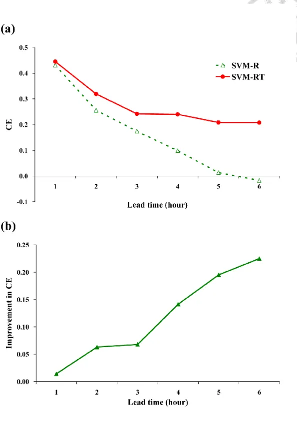
To highlight the influence of typhoon characteristics on rainfall forecasting, we focus on the performance comparison between SVM-R and SVM-RT. As shown in Fig.
3.6(a), the CE values of both SVM-R and SVM-RT decrease with increasing forecast lead-time. However, the CE values of SVM-R decrease more rapidly than those of SVM-RT. The results show that SVM-RT forecasts rainfall depth more accurately than SVM-R, especially for long lead time forecasting. For 1- to 3-h lead time forecasts, the CE values of SVM-R and SVM-RT respectively decrease from 0.43 to 0.17 and from 0.44 to 0.24. Then, the performance of SVM-R gets worse and the CE values
34
decrease rapidly from 0.10 to -0.02 for 4- to 6-h lead time forecasts. It is clear that SVM-R cannot yield effective forecasts (i.e. CE<0) when the forecast lead-time is greater than four hours. As to SVM-RT, the performance does not get worse for long lead-time forecasting. For 4- to 6-h lead time forecasts, the CE values only decrease from 0.24 to 0.21. The addition of typhoon characteristics effectively decreases the negative impact of increasing forecast lead-time.
The improvement in CE due to the addition of typhoon characteristics is presented in Fig. 3.6(b). As shown in Fig. 3.6(b), the improvement increases with increasing forecast lead-time. For 1- to 3-h lead time forecasts, the improvement in CE only increases from 0% to 7%. The improvement due to the addition of typhoon characteristics is not very significant for one- to three-hour ahead forecasts. A much greater improvement in CE is obtained for the long lead-time forecasting. The improvement in CE increases from 15% to 23% for 4- to 6-h lead time forecasts.
Obviously, the addition of typhoon characteristics significantly improves the long lead-time forecasting.
35
Figure 3.6 (a) CE values of SVM-RT and SVM-R and (b) the improvement in CE due to the addition of typhoon characteristics
36
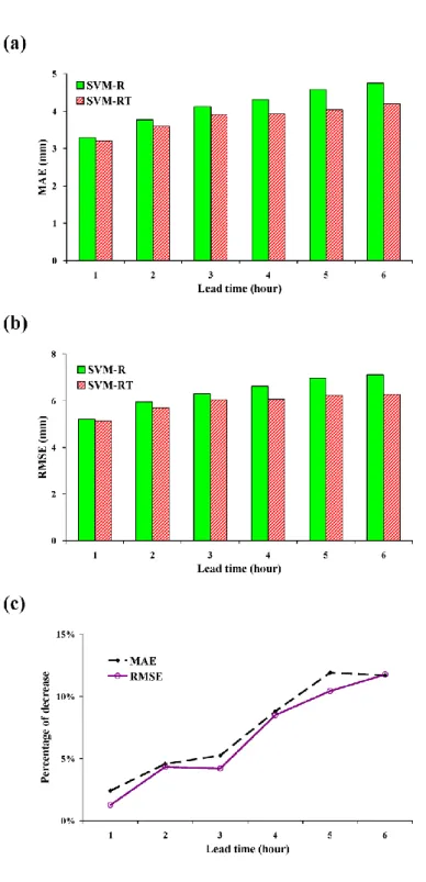
According to the other two performance measures (MAE and RMSE), similar results are also obtained. Fig. 3.7(a) and 3.7(b) show that both the MAE and RMSE values of SVM-R increase more rapidly than those of SVM-RT. Fig. 3.7(c) presents the percentages of decrease in MAE and RMSE due to the addition of typhoon characteristics. For 1- to 3-h lead time forecasts, SVM-RT respectively decreases MAE and RMSE values from 2% to 5% and from 1% to 4% as compared to SVM-R.
The percentages of decrease in MAE and RMSE values are not very significant.
However, the addition of typhoon characteristics brings a greater decrease in MAE and RMSE values for the long lead time forecasting. As compared to SVM-R, SVM-RT respectively decreases MAE and RMSE values from 9% to 12% and from 8% to 10%
for 4- and 6-h lead time forecasts. Again, the results confirm that typhoon characteristics effectively improve the long lead-time forecasting and decrease the negative impact of increasing forecast lead-time.
37
Figure 3.7 (a) MAE, (b) RMSE values of SVM-RT and SVM-R, and (c) the percentages of decrease in MAE and RMSE due to the addition of typhoon
characteristics
38
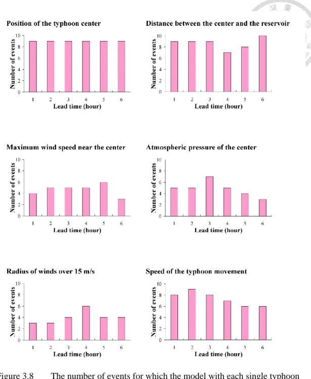
To investigate the influence of each typhoon characteristic on rainfall forecasting, performance comparisons between models with single typhoon characteristic and models without typhoon characteristics (SVM-R) for 10 testing events are made. The number of events for which the model with single typhoon characteristic yields a higher CE value than SVM-R is presented in Fig. 3.8. Though only single typhoon characteristic is added to the model, improvement in performance could still be obtained for at least 40% of total events. The results show that each collected typhoon characteristics are effective for typhoon rainfall forecasting. Among all collected typhoon characteristics, the position of typhoon center is the most effective typhoon characteristic for improving rainfall forecasting. The addition of the position of typhoon center improves forecasting performance for 90% of total events. In addition, the distance between the center and the reservoir and the speed of the typhoon movement improves forecasting performance for 87% and 73% of total events, respectively. It is noted that the aforementioned three typhoon characteristics (the position of typhoon center, the distance between the center and the reservoir, and the speed of the typhoon movement) are highly related to the typhoon path. Thus, more accurate forecasts of typhoon path may be required to further improve the accuracy level of typhoon rainfall forecasting.
39
Figure 3.8 The number of events for which the model with each single typhoon characteristic yields a higher CE value than SVM-R
40
3.3 Summary
To provide effective forecasts of hourly rainfall for supporting reservoir operation systems during typhoons, more accurate, robust and efficient models are proposed in this chapter. For this purpose, SVMs, instead of BPNs, are adopted to construct forecasting models. In addition to using SVMs instead of BPNs, typhoon characteristics are added to the proposed model to further improve the long lead-time forecasting. An application is conducted to demonstrate the superiority of the proposed models. Firstly, the forecasting performance of SVM-based models is compared with that of BPN-based models. The results clearly show that SVM-based models yield acceptably accurate forecasts for 1- to 6-h lead time forecasts, but BPN-based models produce effective 1- to 2-h lead time forecasts only. Hence SVM-based models perform much better than BPN-based models. In addition, the other two major advantages of SVMs over BPNs are the robustness and the efficiency, which are very important but have received little attention in the hydrologic domain.
Representative examples given in this paper indicate that SVM-based models are more robust and the development of SVM-based models is much more efficient.
Finally, the comparison between the SVM-based models with and without typhoon characteristics is presented to confirm that the addition of typhoon characteristics
41
effectively decrease the negative impact of increasing forecast lead-time and significantly improves the forecasting performance, especially for long lead-time forecasting. In conclusion, the proposed SVM-based models are more accurate, robust and efficient than existing BPN-based models, and the typhoon characteristics should be used as input to the typhoon rainfall forecasting models for long lead-time forecasting.
The proposed SVM-based models with typhoon characteristics are recommended as an alternative to the existing models. The proposed modeling technique is useful to improve the hourly typhoon rainfall forecasting and is suitable to be integrated with reservoir operation systems. The proposed modeling technique is also expected to be helpful to support flood, landslide, debris flow and other disaster warning systems.
42
Chapter 4 Typhoon flood forecasting using integrated SVM
4.1 Model development 4.1.1 Model construction
The architecture of the proposed two-stage SVM-based model (named SVM-QRf herein) is illustrated in Fig. 4.1a. In the first stage, the rainfall forecasting module, which is developed based on SVMs, is used to pre-process the typhoon information (namely, typhoon characteristics and rainfall) and to produce rainfall forecasts. Then in the second stage, the forecasted rainfall and the observed runoff are used as input to the flood forecasting module which is also developed based on SVMs. For comparison with the proposed model, another SVM-based flood forecasting model (named SVM-QRT) with observed runoff, rainfall and typhoon characteristics is also constructed. It should be noted that rainfall and typhoon characteristics are directly used as input to SVM-QRT without any processing (Lin et al., 2009a). The architecture of SVM-QRT is illustrated in Fig. 4.1b.