Option Pricing with Higher Moments Consideration

(1)

東吳大學經濟學系

博士論文

指導教授：林忠機博士

Option Pricing with Higher Moments Consideration

研究生：謝長杰撰

中華民國 1 0 3 年 1 2 月

(2)

I

Abstract

This dissertation consists of three essays, one of which examines if it is possible to find the characteristic that can be adapted to abnormal fluctuations and unpredictable cluster effects in the real world by refining the traditional covered-call strategy with stochastic volatility in order to improve this strategy under the Black and Scholes model (1973). Since the distribution of the return of the target asset in the real world is highly likely to be left-skewed and leptokurtic, it will influence the accuracy of the option pricing; otherwise, the basic hypothesis of the return of the target asset is normally distributed, such as in the simple BS model, the GARCH pricing model, and many other stochastic volatility models. Therefore, this study adopts three approximations to price - Gram-Charlier approximate solution, Edgeworth approximate solution, and Shaddlepoint approximate solution - in order to take skewness and kurtosis into account. The first two approximate solutions are derived from the Approximation of Taylor Series Expansion. The laster solution is derived from the asymptotics method from the concept in statistics.

Under the consideration of skewness and kurtosis in the pricing model of European options, this paper introduces three analytic solutions and their detailed derivations. First, this paper compares these three approximations with numerical simulations to show the possible bad effects mentioned by other scholars in the past literature. The bad effect entails out of the possible range between zero to one in the probability density function. Second, this paper compares the accuracy among these three approximations by the benchmark Merton jump model (1976).

Third, because American option pricing does not possess a closed-form and is not easy to price, many scholars have evaluated the price of American options in many different ways. This paper presents most of the different American option pricing methods that have been introduced in the literature and looks to further improve the American option pricing model introduced by Kallast and Kivinukk

(3)

II

(2003).¹ This paper integrates the three approximations into Kim’s integral equations and evaluates their accuracy with Monte Carlo simulation.

Keywords: Edgeworth, Gram-Charlier, Shaddlepoint, Skewness, Kurtosis

1 Their paper is an extension of “the analytic valuation of American options”, which was proposed by Kallast and Kivinukk in 2003.

(4)

III

Figure Contents

Figure 2.1TAIFEX options' historical volumes (2001~2010). ... 6

Figure 2.2TAIFEX futures (Feb-2004~Nov-2011). ... 8

Figure 2.3Call premium (as a percentage of futures) (Feb-2004~Nov-2011). ... 11

Figure 2.4Moneyness of the dynamic portfolios and implied volatility under the Black model (Feb-2004~Nov-2011). ... 11

Figure 2.5Moneyness of the dynamic portfolios under the Heston model (Feb-2004~Nov-2011). ... 12

Figure 2.6The tradeoff between return and SD for naked futures, conventional covered-call, and dynamic covered-call strategies. ... 15

Figure 2.7Cumulative total return (3% OTM, and prob.=30%). ... 21

Figure 2.8Cumulative total return (1% OTM, and prob.=20%).. ... 23

Figure 2.9Cumulative total return (6% OTM, and prob.=49%).. ... 23

Figure 3.1Convergence of the Gram-Charlier Approximation ... 34

Figure 3.2Convergence of the Edgeworth Approximation ... 35

Figure 3.3Convergence of the Saddlepoint Approximation ... 36

Figure 4.1Exercise boundary (different strike prices) ... 55

Figure 4.2Exercise boundary (different maturities) ... 56

Figure 4.3Exercise boundary (different riskless rates) ... 56

Figure 4.4Exercise boundary (different volatilities) ... 57

Figure 4.5Exercise boundary (Non-Normal) ... 58

(7)

VI

Table Contents

Table 2.1 Overall monthly performance of different fixed moneyness

(Feb-2004~Jan-2012). ... 13

Table 2.2 Overall monthly performances of different exercise probabilities under the Black model (Feb-2004~Jan-2012). ... 14

Table 2.3 Overall monthly performances of different exercise probabilities under the Heston model (Feb-2004~Jan-2012). ... 15

Table 2.4 Fixed strike strategy under different market conditions. ... 17

Table 2.5 Dynamic (Black) strike strategy under different market conditions. . 18

Table 2.6 Dynamic (Heston) strike strategy under different market conditions. 19 Table 2.7 Performance under conventional strategy and dynamic strategies (Black and Heston models). ... 20

Table 3.1 Performance of accuracy ... 36

Table 3.2 Mean square errors under Black's formula and three approximations38 Table 3.3 Performance of improvement ability among three approximations ... 39

Table 4.1 Descriptive statistics of the random numbers ... 54

Table 4.2 Sensitivity analysis depending on strike prices ... 59

Table 4.3 Sensitivity analysis depending on time periods ... 60

Table 4.4 Sensitivity analysis depending on riskless interest rates ... 61

Table 4.5 Sensitivity analysis depending on volatilities ... 62

Table 4.6 Relative differences and relative efficiencies ... 63

(8)

1

Chapter 1 Introduction

1.1 Background

The concept of the option pricing model was provided by Black and Scholes in 1976, but later researchers found that certain limitations were incurred by their assumptions. First, the price of the underlying security undergoes a Geometric Brownian Motion, which has a lognormal distribution. Second, the risk-free interest rate and volatility are constants in the original model.

In the past two decades many studies have shown empirical evidence that the Black-Scholes model overprices options that are at-the-money and also underprices options that are deeply out-of-money and deeply in-the-money. The word “fat-tailed” is a common concept among modern investors, i.e. a distribution that has a higher probability of huge changes in the price of underlying than the prediction by lognormal distribution. During the financial crisis of 2007-2008, panic among investors produced unreasonable behavior, resulting in them selling down holdings in the financial markets whether the stocks had reasonable values or not. The popular term for such an extreme change is the so-called black swan effect. This phenomenon is rarely seen, but when it occurs, it brings about serious impacts. In fact, the black swan effect has a higher possibility of occurring in the financial markets than the Black and Scholes model predicts.

In the real world of stock options trading, one can often find higher implied volatility in put options than in call options. Obviously, investors always dislike taking a loss in stock markets, and so they need to hedge their risk when owning the stocks. Naturally, people are always concerned about an unexpected event that could suddenly occur, which would affect them negatively.

(9)

2

1.2 Motivation

The market price of stock options is composed of two layers. One is the result closely derived from the mathematical model, and the other is the unreasonable price that reflects unreasonable behavior due to unexpected events.

Behavioral finance has been a top issue in recent decades. It is investors’

buying-and-selling behaviors in the financial markets. The prices of derivative products reflect their attitudes toward the market and any irrationally unexpected behaviors.

It is very interesting to dig out the information extracted from options prices in the real financial markets. Indeed, we can even make predictions more precise if we have more market information. Many researchers have suggested alternatives to the Black and Scholes model, including stochastic volatility models and jump-diffusion models. In stochastic volatility models the futures volatility of a stock price is uncertain, while in jump-diffusion models the stock price experiences occasional jumps rather than continuous changes. Because the surface of financial markets is more socialized than mathematical, any one specific model cannot apply to all environments. Hence, we shall attempt in this research to try and understand how the return distribution of the underlying stock looks in the real world.

This paper assumes the futures index has stochastic volatility behaviors. We adopt stochastic volatility to replace the Black and Scholes model in the traditional covered-call strategy in order to verify if stochastic volatility is closer to irrational fluctuations in the markets. This paper further derives the European option and American option, which have skewness and kurtosis effects.

1.3 Framework

Chapter 2 examines the performances of a conventional strategy and dynamic covered-call strategies, including constant and stochastic volatility environments in Taiwan. In accordance with the prior literature, the covered-call

(10)

3

strategy may roughly boost a portfolio return under some specific moneyness.

The monthly return of the conventional covered-call strategy has slightly more profit than the naked futures buy-and-hold strategy on average. The dynamic strategies adjust the moneyness based on different exercise probabilities under constant volatility and stochastic volatility. This study points out that the advantage of the dynamic strategy under stochastic volatility is more obvious than said strategy under constant volatility or a conventional strategy.

Chapter 3 presents three approximate solutions. Black and Scholes (1973) assumed that the return of a stock follows a Geometric Brownian Motion.

However, many empirical research studies pointed out that biases exist in deep in-the-money and deep out-the-money, such as volatility smiles. Other model risks are also generated when the distribution is fat-tail in practical applications.

Hence, we can reduce pricing errors if we estimate that the distribution of the return on the asset is more accurate. This research compares three kinds of approximate solutions: the Saddlepoint method first supposed by Lugannani and Rice (1980), and the Gram-Charlier and Edgeworth methods in pricing error.

The conclusions are as follows. First, the range of convergence performs better in the Saddlepoint method than in the other two methods under the scenarios of different skewness and kurtosis using the Monte Carlo simulation. Second, the performance of accuracy is better when using the Saddlepoint method versus the other two methods given the benchmark Merton (1976) jump model. Third, the Saddlepoint method results in the lowest pricing errors of these three methods using empirical data from the Taiwan futures exchange.

Chapter 4 focuses on American option pricing. First, this chapter introduces most of the different American option pricing methods that have been mentioned in the literature. This chapter integrates the Kim integral equations with skewness and kurtosis.

This research is presented in such a way that any of the following 3 chapters can be read independently. In this case, Chapter 2 mainly discusses the performances of different trading strategies. This paper then looks to develop

(11)

4

another model that contains the effects of skewness and kurtosis in Chapters 3 and 4. Chapter 3 mainly focuses on European options, while Chapter 4 targets American options. The content of Chapter 2 has been published in Soochow Journal of Economics and Business in Taiwan in 2014.

(12)

5

Chapter 2 Empirical Performance of Covered-Call Strategy under Stochastic Volatility in Taiwan

2.1 Introduction

The Black-Scholes model is the most popular option pricing model in the world, but there are still some shortcomings. Previous research pointed out the case that the option price is lower than the Black-Scholes price when the stock price is quite close to the exercise price, and that the option price is higher than the Black-Scholes price when the stock price is deeply in- or out-of-the-money.

Hence, we can expect that the price bias will be more severe in a highly fluctuating market, such as emerging markets.

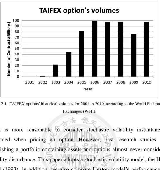
The emerging financial market of Taiwan has grown quite rapidly, especially in the futures market. Established in 1998, the Taiwan futures exchange (TAIFEX) is one of the fastest growing options market in the world (see Figure). TAIFEX options’ volume is ranked the sixth largest market around the world in 2010 according to a report by the World Federation of Exchanges (WFE).

(13)

6

Figure 2.1 TAIFEX options’ historical volumes for 2001 to 2010, according to the World Federation of Exchanges (WFE).

It is more reasonable to consider stochastic volatility instantaneously embedded when pricing an option. However, past research studies about establishing a portfolio containing assets and options almost never consider the volatility disturbance. This paper adopts a stochastic volatility model, the Heston model (1993). In addition, we also compare Heston model’s performance with the Black-Scholes model’s and expect to get more precise forecasting option prices in TAIFEX.

A covered-call (buy-write) option trading strategy, which is a portfolio combining one unit of the long underlying assets while writing one call option, has been studied in the previous literature in order to assess its performance. This trading strategy is the simplest concept extended from the Capital Asset Pricing Model (CAPM), which is used to hold a negative correlation between the asset and its derivative to improve returns and to reduce risks. The trading strategy is for the holders to receive a premium when they sell a call option; at the same time, the premium can reduce the cost of a single long position of the underlying asset. The premium amount depends on the extension of the OTM (out-of-money) conditions. Holders of this trading strategy will receive a greater premium as the

0 10 20 30 40 50 60 70 80 90 100

2001 2002 2003 2004 2005 2006 2007 2008 2009 2010

Number of Contracts(Billions)

Year

TAIFEX option's volumes

(14)

7

option exercise price becomes closer to the current underlying asset. Another important factor is the underlying asset’s volatility, which represents the fluctuating degree of the underlying asset. Therefore, choosing the appropriate moneyness is a key to the performance of building a covered-call portfolio.

Che and Fung (2011) used the conventional buy-write (covered-call) strategy and a dynamic buy-write strategy to test the performance on Hang Seng Index (HSI) in Hong Kong. They adopted HSI futures to substitute for HSI in order to reduce the impact of transactional cost and execution problems. They found that both strategies outperform the naked futures position. Although the dynamic strategy uses various risk-adjusted measures, which usually have lower returns than the conventional fixed strike strategy, the dynamic strategy outperforms the fixed strategy when the market is moderately volatile or is sharply rising market.

Figelman (2008) introduced a simple theoretical framework that allows decomposing the observed historical performance of a covered-call strategy into three market components: risk-free rate, equity risk premium, and implied-realized volatility spread. He pointed out that a covered-call strategy is highly correlated with an equity market index (S&P 500), especially in a bull market. Hill et al. (2006), Feldman and Dhruv (2004), and Whaley (2002) also investigated covered-call strategies on the S&P 500, but did not obtain strong evidence to explain that covered-call strategies provide better performance than a naked futures position. Nevertheless, they concluded that covered-call strategies can effectively reduce risks (standard derivation).

This study extends the works of Che and Fund (2011) and Figelman (2008) to investigate the performance of a covered-call strategy in TAIFEX. We divide the market into different situations (rising (bullish) or falling (bearish); sharply or moderately, see Figure 2.2) and examine the performances of a conventional strategy and dynamic covered-call strategies including constant and stochastic volatility environments in Taiwan.

The different scenarios should allow us to know whether the strategies work

(15)

8

well or not. Here, we use subjective judgements to define different scenarios, just like Figelman (2008) did. Hence, we define that periods 1, 4, and 8 represent sharply falling, periods 3, 5, and 7 represent sharply rising, period 2 represents moderately rising, and period 6 is moderately falling.

Figure 2.2 TAIFEX futures for Feb-2004 to Nov-2011.

The rest of this section is organized as follows. Section 2.2 introduces the covered-call option trading strategies as well as the constant volatility and stochastic volatility futures option pricing models. Section 2.3 describes the data and defines four different market situations. The last section is the conclusion.

2.2 Modified Heston Model

A covered-call trading strategy in this paper is built to buy index futures and simultaneously sell short European calls. Therefore, the volatility of the underlying futures and option exercise price will affect the performance of the covered-call trading strategy. When the volatility of the underlying futures increases, the income from the short sale from the call options will increase. As the option is close to the ATM (at the money) condition, the income rises.

(16)

9

Building the covered-call strategy involves a short sale position from futures call options, which involve the option pricing models. We first assume the volatility of underlying futures is constant, in accordance with the Black (1976) model, shown in equation (2.1), which will be used for constructing the short sale from a call option position.

c = F₀N(d₁)− XN(d₂) (2.1)

Here, d₁ = (𝑙𝑛(F₀⁄ ) + 𝜎X ²𝑇/2)/𝜎√𝑇 , and d2 = (𝑙𝑛(F₀⁄ ) − 𝜎X ²𝑇/2)/𝜎√𝑇 . Moreover, F₀ is the price of underlying futures; X is the exercise price; T is the time to maturity in years; and c and p represent call and put options, respectively.²

The stochastic volatility environment, as in the Heston (1993) model, shown in equations (2.2) to (2.4), will be used for constructing the short sale from a call option position. We define equation (2.4) as a modified Heston model, because we use the underlying futures index to replace the stock index. There is no discount factor in the right-hand side of the minus sign.

dx_𝑡 = [𝑟 −¹

2𝑣_𝑡] dt+√𝑣_𝑡d𝑧_1,𝑡 (2.2) d𝑣_𝑡 = 𝑘 × [𝜃 − 𝑣_𝑡]dt+σ × √𝑣_𝑡d𝑧_2,𝑡 (2.3) c = F₀× P₁− X × P₂, (2.4) where θ is the long-run mean of the variance; 𝑘 is a mean reversion parameter; σ is the volatility of volatility; F is the futures price; X is the exercise price of the call option; r is the risk-free interest rate; and v is volatility. The quantities P₁ and P₂ are the probabilities that will be exercised by the call option, conditional on the log of the last futures price, x_𝑇 = ln (𝐹_𝑇), and on the last volatility v_𝑇. The

2The put option can be derived from put-call parity.

(17)

10

risk-neutral dynamics are expressed as equations 2.2 and 2.3, and 𝑧₁ and 𝑧₂ are Weiner processes. The other details are provided in Appendix A.

The return from a covered-call is derived as:

Return = F_T− F₀

F₀ +C(X)

F₀ −𝑀𝑎𝑥(F_T− X , 0)

F₀ ,

where F_T is the last settlement price. For instance, if you are merely long in a futures contract, it is possible for you to gain the profit once the futures index goes up, while you will incur a loss for sure when the futures index falls. There is unlimited profit or loss when you only hold a naked long futures or only a naked short futures.

In the real trading world, the price of underlying stock is impossible to fluctuate dramatically in a short time. Experienced traders are willing to take a limited risk in order to produce additional profits. Alternatively, many traders look for opportunities on options that they feel are overvalued and will offer a good return. Hence, the covered call strategy is the most considerate by traders. The covered call strategy plays the role of the seller in the options and exhibits limited risk, because the underlying stock or futures is already in the portfolio. The term

“covered” means that the unlimited loss will be covered in the event that the call option goes in the money and will be exercised.

How to select the adequate exercise price (or moneyness level) is the key point for whether call options will be exercised or not. Generally, the greater the out-of-money exercise price you choose, the more profit and risk you will expect.

Obviously, there is a trade-off problem, which is mapping with the second and third terms in the right-hand side of the above equation.

Volatility is the main factor that affects the call price. Hence, the jargon “trade vol.” describes that the traders like to sell options with relatively high volatility and buy options with relatively low volatility. The assumptions of the Black and Scholes model and the Heston model have the distinctive characteristics to

(18)

11

describe volatility of a stock. Basically, we expect the Heston model to react more easily under volatility than the Black and Scholes model does. In other words, the Heston model can choose the adequate exercise price theoretically.

In this study we try to find the evidences if the Heston model perform well.

For this purpose, the selected exercise price is divided into the fixed ratio model and the dynamic adjustment model. The rewards of fixed ratio models consist of a traditional fixed exercise price and futures price in the beginning of the period.

We study the exercise price for the degree of difference from 1% to 6% OTM during four specific ranges.

Figure 2.3 conveniently illustrates the specific moneyness (ATM, and 3%

and 6% OTM). We can see a clear change in the price of the option premium.

The dynamic adjustment model exhibits constructive dynamic parts of the fixed compliance probability. This study, in addition to the construction of Black’s (1976) futures option pricing model for the fixed compliance probability and volatility, back-steps the specific exercise price.

We then follow the same seven distinct probabilities of compliance cases, which were set in Che and Fund’s (2011) research. The results of different moneyness trends are shown in Figure 2.4. For the purpose of succinctness, the exercise probabilities 17%, 30%, and 49% stand for all seven distinct probabilities ).

This study also extends the Heston stochastic volatility model (1993) with the optimization techniques for deriving the in-the-money probability P₂. The representative moneyness trends are in Figure 2.5.

(19)

12

Figure 2.3 Call premium (as a percentage of futures) for Feb-2004 to Nov-2011.

Figure 2.4 Moneyness of the dynamic portfolios and implied volatility under the Black model for Feb-2004 to Nov-2011.

(20)

13

Figure 2.5 Moneyness of the dynamic portfolios under the Heston model for Feb-2004 to Nov-2011.

Call options are used as the short position in Taiwan index options (TXO).

In this study, the process is to sell the option contracts in the past month and hold to maturity. According to the model of Che and Fung (2011), in order to reduce the problems of dividends, hedging, transaction costs, and non-synchronous trading, we use Taiwan’s stock market futures (TAIFEX) to replace the Taiwan Stock Index.³.

2.3 Empirical Test

2.3.1 Under All Period Market Conditions

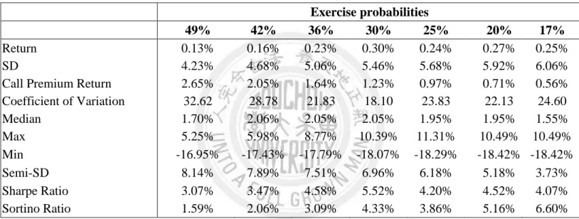
According to the models, Tables 2.1 to 2.3 show the fixed implementation price strategy, dynamic adjustment strategy in compliance probability, risk values, and descriptive statistics. From Feb-2004 to Nov-2011, the monthly

3In the original Heston’s model, the underlying asset is the stock price. We use the futures index to replace the stock index in order to consider the time consistency compared to options and the Heston model is comparable with the Black model.

(21)

14

average return for a simple buy-and-hold strategy is 0.32%.

In covered-call strategies, when the moneyness is deeper OTM, the short position of a call will receive fewer premiums. Generally, the short position of 3% to 6% OTM call options will increase the monthly total return. The risk will be smaller than the naked futures’ position. Finally, whether we use the Sharpe Ratio or the Sortino Ratio as the performance indicators, the short position of a 6% OTM call option can get the best performance, significantly enhance return, and reduce the risk.

Table 2.1 Overall monthly performance of different fixed moneyness for Feb-2004 to Jan-2012.

Moneyness (percentage of out-of-money ) Naked

Futures 1% 2% 3% 4% 5% 6%

Return 0.32% 0.19% 0.25% 0.34% 0.37% 0.40% 0.43%

SD 6.75% 4.62% 4.89% 5.20% 5.48% 5.72% 5.91%

Call Premium Return 2.09% 1.71% 1.35% 1.09% 0.86% 0.69%

Coefficient of Variation 20.93 23.75 19.48 15.31 14.94 14.27 13.69

Median 0.98% 2.09% 2.38% 2.05% 2.05% 1.66% 1.39%

Max 15.65% 5.98% 5.98% 7.30% 7.34% 8.77% 8.91%

Min -18.72% -17.43% -17.79% -18.07% -18.07% -18.29% -18.42%

Semi-SD 4.53% 5.13% 5.77% 6.52% 7.30% 8.12% 8.95%

Sharpe Ratio 4.78% 4.21% 5.13% 6.53% 6.69% 7.01% 7.30%

Sortino Ratio 7.12% 3.80% 4.35% 5.21% 5.02% 4.94% 4.82%

Table 2.2 and Table 2.3 show the results of dynamic adjustment covered-call, respectively, under the Black (1976) model and under the Heston (1993) model.

Both implied volatilities are calculated by using all day-end information, excluding any volume under 100 contracts. In the Heston model, we use the method of exhaustion to obtain the optimal parameters in a given lower bound [0.01, 0.01, -1, 0.01, and 0.01] and upper bound [0.6, 0.6, 1, 5, and 0.6].

(representing the volatility of variance, current variance, rho, kappa, and the long-run mean of the variance, respectively.)

In the Black (1976) model, the rewards in all seven compliance probabilities

(22)

15

from 17% to 49% are less than the naked futures’ position. However, there is still an advantage to choose the exercised probability of around 30% in order to reduce any fluctuation in the return. The Heston (1993) model significantly improves the performance of the remuneration. Apparently, the dynamic covered-call strategies under Black (1976) perform less than the naked futures’

position. The Heston (1993) model is much closer to the actual cases than the Black (1976) model.

Table 2.2 Overall monthly performances of different exercise probabilities under the Black model for Feb-2004 to Jan-2012.

Exercise probabilities

49% 42% 36% 30% 25% 20% 17%

Return 0.13% 0.16% 0.23% 0.30% 0.24% 0.27% 0.25%

SD 4.23% 4.68% 5.06% 5.46% 5.68% 5.92% 6.06%

Call Premium Return 2.65% 2.05% 1.64% 1.23% 0.97% 0.71% 0.56%

Median 1.70% 2.06% 2.05% 2.05% 1.95% 1.95% 1.55%

Max 5.25% 5.98% 8.77% 10.39% 11.31% 10.49% 10.49%

Min -16.95% -17.43% -17.79% -18.07% -18.29% -18.42% -18.42%

Semi-SD 8.14% 7.89% 7.51% 6.96% 6.18% 5.18% 3.73%

Sharpe Ratio 3.07% 3.47% 4.58% 5.52% 4.20% 4.52% 4.07%

Sortino Ratio 1.59% 2.06% 3.09% 4.33% 3.86% 5.16% 6.60%

(23)

16

Table 2.3 Overall monthly performances of different exercise probabilities under the Heston model from Feb-2004 to Jan-2012.

Exercise probabilities

49% 42% 36% 30% 25% 20% 17%

Return 0.26% 0.31% 0.39% 0.35% 0.39% 0.44% 0.40%

SD 4.61% 4.94% 5.31% 5.57% 5.85% 6.10% 6.18%

Call Premium Return 2.20% 1.73% 1.38% 1.09% 0.82% 0.63% 0.53%

Median 2.11% 2.34% 2.05% 2.05% 1.66% 1.55% 1.39%

Max 5.98% 7.30% 8.70% 9.79% 10.63% 12.35% 12.15%

Min -17.43% -17.79% -18.07% -18.07% -18.29% -18.29% -18.42%

Semi-SD 8.37% 8.07% 7.64% 7.08% 6.31% 5.28% 3.78%

Sharpe Ratio 5.58% 6.18% 7.27% 6.36% 6.62% 7.13% 6.50%

Sortino Ratio 3.07% 3.78% 5.05% 5.01% 6.14% 8.25% 10.62%

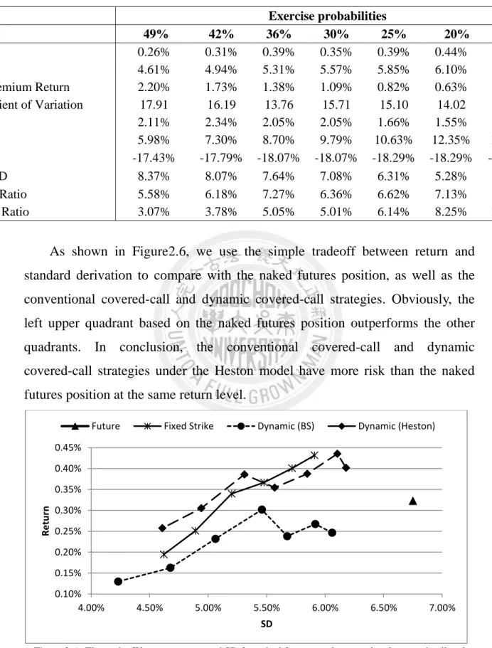
As shown in Figure2.6, we use the simple tradeoff between return and standard derivation to compare with the naked futures position, as well as the conventional covered-call and dynamic covered-call strategies. Obviously, the left upper quadrant based on the naked futures position outperforms the other quadrants. In conclusion, the conventional covered-call and dynamic covered-call strategies under the Heston model have more risk than the naked futures position at the same return level.

Figure 2.6 The tradeoff between return and SD for naked futures, and conventional covered-call and dynamic covered-call strategies.

0.10%

0.15%

0.20%

0.25%

0.30%

0.35%

0.40%

0.45%

4.00% 4.50% 5.00% 5.50% 6.00% 6.50% 7.00%

Return

SD

Future Fixed Strike Dynamic (BS) Dynamic (Heston)

(24)

17

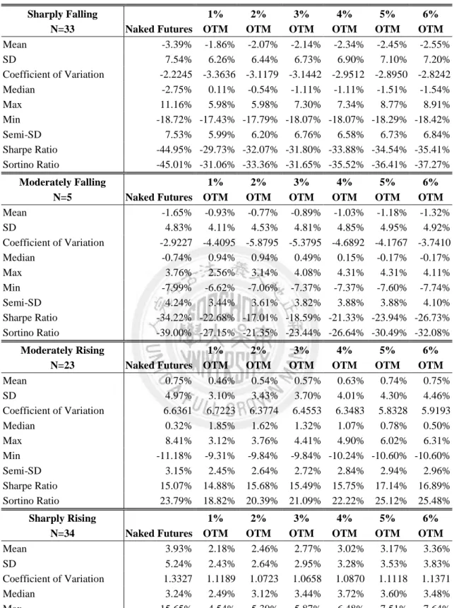
2.3.2 Under Different Market Conditions

Financial products in different market conditions tend to behave differently.

This study refers to the setting of Che and Fund (2011), dividing Taiwan’s market into four conditions: sharply falling, moderately falling, sharply rising, and moderately rising. Tables 2.4 to 2.6 show the results.

For the average return of seven probabilities, in a sharply falling market, selling options close to ATM can receive more premiums, and the dynamic adjustment covered-call (under both the Black and Heston models) strategies can effectively reduce losses. In a moderately falling market, the dynamic covered-call strategy is better than the conventional strategy under the Black model, and the performance of the Heston model is worse than the Black model.

However, in Taiwan there are only four months with a moderately falling situation during our study’s time period. Even so, the Heston model is still better than executing a naked futures’ position.

In a sharply rising market, all the covered-call strategies are worse than the naked futures strategy, however, if we evaluate the performance under the Sharpe ratio, the covered-call strategies are better than using naked futures, as they can effectively reduce risks. We are able to still point out that the Heston model is better than the Black model in the moderately rising market.

We note that the Black and Heston models choose the same probabilities of the closest ATM in a sharply falling market and those of the deeply OTM in a sharply rising market. The most interesting part is that the Heston model chooses to receive a higher premium than the Black model in the case of a moderately falling market and to receive fewer premiums than the Black model in the moderately rising situation in order to reduce the probability of exercise. Overall, this is the reason why the Heston model performs better than the Black model.

(25)

18

Table 2.4 Overall monthly performance of a fixed strike strategy under different market conditions.

Sharply Falling 1% 2% 3% 4% 5% 6%

N=33 Naked Futures OTM OTM OTM OTM OTM OTM

Mean -3.39% -1.86% -2.07% -2.14% -2.34% -2.45% -2.55%

SD 7.54% 6.26% 6.44% 6.73% 6.90% 7.10% 7.20%

Coefficient of Variation -2.2245 -3.3636 -3.1179 -3.1442 -2.9512 -2.8950 -2.8242

Median -2.75% 0.11% -0.54% -1.11% -1.11% -1.51% -1.54%

Max 11.16% 5.98% 5.98% 7.30% 7.34% 8.77% 8.91%

Min -18.72% -17.43% -17.79% -18.07% -18.07% -18.29% -18.42%

Semi-SD 7.53% 5.99% 6.20% 6.76% 6.58% 6.73% 6.84%

Sharpe Ratio -44.95% -29.73% -32.07% -31.80% -33.88% -34.54% -35.41%

Sortino Ratio -45.01% -31.06% -33.36% -31.65% -35.52% -36.41% -37.27%

Moderately Falling 1% 2% 3% 4% 5% 6%

Mean -1.65% -0.93% -0.77% -0.89% -1.03% -1.18% -1.32%

SD 4.83% 4.11% 4.53% 4.81% 4.85% 4.95% 4.92%

Median -0.74% 0.94% 0.94% 0.49% 0.15% -0.17% -0.17%

Max 3.76% 2.56% 3.14% 4.08% 4.31% 4.31% 4.11%

Min -7.99% -6.62% -7.06% -7.37% -7.37% -7.60% -7.74%

Semi-SD 4.24% 3.44% 3.61% 3.82% 3.88% 3.88% 4.10%

Sharpe Ratio -34.22% -22.68% -17.01% -18.59% -21.33% -23.94% -26.73%

Sortino Ratio -39.00% -27.15% -21.35% -23.44% -26.64% -30.49% -32.08%

Moderately Rising 1% 2% 3% 4% 5% 6%

Mean 0.75% 0.46% 0.54% 0.57% 0.63% 0.74% 0.75%

SD 4.97% 3.10% 3.43% 3.70% 4.01% 4.30% 4.46%

Median 0.32% 1.85% 1.62% 1.32% 1.07% 0.78% 0.50%

Max 8.41% 3.12% 3.76% 4.41% 4.90% 6.02% 6.31%

Min -11.18% -9.31% -9.84% -9.84% -10.24% -10.60% -10.60%

Semi-SD 3.15% 2.45% 2.64% 2.72% 2.84% 2.94% 2.96%

Sharpe Ratio 15.07% 14.88% 15.68% 15.49% 15.75% 17.14% 16.89%

Sortino Ratio 23.79% 18.82% 20.39% 21.09% 22.22% 25.12% 25.48%

Sharply Rising 1% 2% 3% 4% 5% 6%

Mean 3.93% 2.18% 2.46% 2.77% 3.02% 3.17% 3.36%

SD 5.24% 2.43% 2.64% 2.95% 3.28% 3.53% 3.83%

Median 3.24% 2.49% 3.12% 3.44% 3.72% 3.60% 3.48%

Max 15.65% 4.54% 5.39% 5.87% 6.48% 7.51% 7.64%

Min -9.60% -8.30% -8.63% -8.92% -9.15% -9.31% -9.31%

Semi-SD 2.10% 1.59% 1.64% 1.74% 1.82% 1.85% 1.89%

Sharpe Ratio 75.03% 89.37% 93.26% 93.83% 92.00% 89.95% 87.94%

Sortino Ratio 186.89% 136.97% 149.41% 159.44% 165.77% 171.64% 177.80%

(26)

19

Table 2.5 Overall monthly performance of a dynamic (Black) strike strategy under different market conditions.

Sharply Falling

49% 42% 36% 30% 25% 20% 17%

N=33

Mean -1.62% -1.99% -2.12% -2.33% -2.56% -2.81% -2.90%

SD 5.89% 6.34% 6.82% 7.19% 7.34% 7.41% 7.52%

Median 0.88% -0.04% -1.11% -1.36% -1.67% -2.24% -2.45%

Max 5.25% 5.98% 8.77% 10.39% 11.31% 10.49% 10.49%

Min -16.95% -17.43% -17.79% -18.07% -18.29% -18.42% -18.42%

Semi-SD 5.64% 6.10% 6.44% 6.74% 6.94% 7.14% 7.24%

Sharpe Ratio -27.47% -31.34% -31.10% -32.42% -34.90% -37.84% -38.54%

Sortino Ratio -28.66% -32.59% -32.96% -34.59% -36.93% -39.32% -40.03%

Moderately Falling

49% 42% 36% 30% 25% 20% 17%

N=5

Mean -0.84% -0.67% -0.49% -0.79% -0.85% -1.10% -1.20%

SD 3.64% 4.19% 4.60% 4.77% 4.75% 4.76% 4.71%

Median 1.56% 0.94% 0.94% 0.49% 0.15% 0.15% -0.17%

Max 1.93% 3.14% 4.08% 4.31% 4.31% 3.98% 3.98%

Min -6.03% -6.62% -6.62% -7.06% -7.06% -7.37% -7.37%

Semi-SD 3.09% 3.32% 3.44% 3.70% 3.70% 3.88% 3.88%

Sharpe Ratio -23.20% -15.97% -10.76% -16.47% -17.98% -23.12% -25.57%

Sortino Ratio -27.36% -20.15% -14.39% -21.25% -23.10% -28.34% -30.99%

Moderately Rising

49% 42% 36% 30% 25% 20% 17%

N=23

Mean 0.46% 0.41% 0.46% 0.55% 0.49% 0.61% 0.56%

SD 2.84% 3.04% 3.25% 3.52% 3.72% 3.98% 4.06%

Median 1.60% 1.61% 1.32% 1.62% 1.62% 1.07% 1.07%

Max 2.72% 3.12% 3.74% 4.41% 4.90% 5.83% 5.83%

Min -8.69% -9.31% -9.84% -9.84% -10.24% -10.60% -10.60%

Semi-SD 2.32% 2.45% 2.54% 2.65% 2.75% 2.85% 2.87%

Sharpe Ratio 16.29% 13.49% 14.11% 15.72% 13.30% 15.33% 13.85%

Sortino Ratio 20.01% 16.77% 18.08% 20.83% 18.00% 21.46% 19.57%

Sharply Rising

49% 42% 36% 30% 25% 20% 17%

N=34

Mean 1.74% 2.20% 2.47% 2.85% 2.94% 3.22% 3.30%

SD 2.11% 2.45% 2.73% 3.14% 3.45% 3.78% 4.02%

Median 1.98% 2.44% 2.72% 3.18% 3.28% 3.46% 3.46%

Max 3.70% 5.39% 5.87% 7.49% 7.51% 8.95% 10.03%

Min -7.92% -8.30% -8.30% -8.63% -8.92% -8.92% -9.15%

Semi-SD 1.47% 1.58% 1.64% 1.77% 1.91% 1.95% 2.02%

Sharpe Ratio 82.78% 89.78% 90.42% 90.56% 85.25% 85.20% 82.02%

Sortino Ratio 118.42% 139.11% 150.76% 160.69% 153.80% 165.10% 163.62%

(27)

20

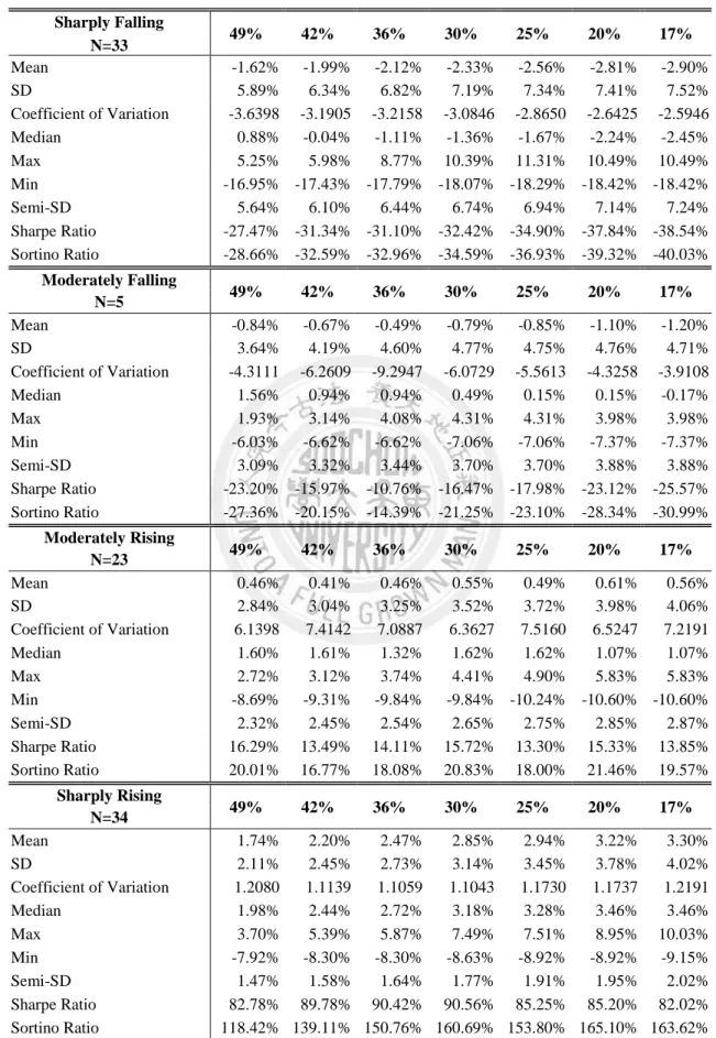
Table 2.6 Overall monthly performance of a dynamic (Heston) strike strategy under different market conditions.

Sharply Falling

49% 42% 36% 30% 25% 20% 17%

N=33

Mean -1.84% -2.05% -2.20% -2.36% -2.53% -2.67% -2.78%

SD 6.24% 6.55% 6.92% 7.19% 7.43% 7.61% 7.62%

Median 0.11% -0.54% -1.11% -1.36% -1.96% -2.24% -2.26%

Max 5.98% 7.30% 8.70% 9.79% 10.63% 12.35% 12.15%

Min -17.43% -17.79% -18.07% -18.07% -18.29% -18.29% -18.42%

Semi-SD 5.97% 6.23% 6.51% 6.73% 6.95% 7.09% 7.17%

Sharpe Ratio -29.55% -31.31% -31.84% -32.76% -34.04% -35.14% -36.44%

Sortino Ratio -30.89% -32.89% -33.85% -35.02% -36.36% -37.73% -38.74%

Moderately Falling

49% 42% 36% 30% 25% 20% 17%

N=5

Mean -0.81% -0.68% -0.94% -0.90% -1.04% -1.10% -1.21%

SD 4.19% 4.38% 4.56% 4.69% 4.89% 4.83% 4.80%

Median 1.56% 0.94% 0.49% 0.15% -0.17% -0.17% -0.34%

Max 2.56% 3.14% 3.14% 4.08% 4.31% 4.31% 4.11%

Min -6.62% -6.62% -7.06% -7.06% -7.37% -7.37% -7.37%

Semi-SD 3.44% 3.44% 3.70% 3.70% 3.88% 3.88% 3.93%

Sharpe Ratio -19.29% -15.59% -20.66% -19.24% -21.20% -22.71% -25.23%

Sortino Ratio -23.54% -19.86% -25.48% -24.39% -26.69% -28.27% -30.82%

Moderately Rising

49% 42% 36% 30% 25% 20% 17%

N=23

Mean 0.53% 0.50% 0.65% 0.52% 0.66% 0.63% 0.66%

SD 3.03% 3.14% 3.47% 3.68% 3.98% 4.14% 4.33%

Median 1.85% 1.94% 1.94% 1.32% 1.07% 0.78% 0.72%

Max 3.12% 3.12% 4.41% 4.90% 5.83% 5.83% 7.38%

Min -9.31% -9.31% -9.84% -10.24% -10.24% -10.60% -10.60%

Semi-SD 2.42% 2.45% 2.59% 2.74% 2.79% 2.90% 2.93%

Sharpe Ratio 17.37% 15.83% 18.63% 14.05% 16.52% 15.11% 15.20%

Sortino Ratio 21.77% 20.30% 24.93% 18.89% 23.57% 21.53% 22.43%

Sharply Rising

49% 42% 36% 30% 25% 20% 17%

N=34

Mean 2.27% 2.61% 2.92% 3.06% 3.24% 3.55% 3.55%

SD 2.38% 2.81% 3.12% 3.37% 3.62% 3.96% 4.04%

Median 2.50% 3.02% 3.18% 3.44% 3.76% 3.60% 3.59%

Max 4.54% 6.42% 7.51% 7.51% 8.77% 9.09% 9.71%

Min -8.30% -8.63% -8.63% -8.92% -9.15% -9.15% -9.31%

Semi-SD 1.60% 1.77% 1.81% 1.91% 1.94% 1.95% 1.97%

Sharpe Ratio 95.62% 92.74% 93.67% 90.75% 89.57% 89.66% 87.90%

Sortino Ratio 141.58% 147.58% 161.09% 160.48% 167.14% 182.12% 179.89%

(28)

21

Table 2.7 The performance under a conventional strategy and dynamic strategies (Black and Heston models).

Total Period 0.17 0.2 0.25 0.3 0.36 0.42 0.49 Average Naked Futures

Fixed Moneyness 0.330%

0.322%

Black Model 0.246% 0.267% 0.238% 0.301% 0.231% 0.162% 0.129% 0.225%

Heston Model 0.401% 0.435% 0.387% 0.354% 0.385% 0.305% 0.257% 0.361%

Sharply Falling 0.17 0.2 0.25 0.3 0.36 0.42 0.49 Average Naked Futures

Fixed Moneyness -2.234%

-3.390%

Black Model -2.899% -2.805% -2.562% -2.331% -2.121% -1.986% -1.617% -2.332%

Heston Model -2.777% -2.674% -2.528% -2.355% -2.203% -2.050% -1.844% -2.347%

Moderately Falling 0.17 0.2 0.25 0.3 0.36 0.42 0.49 Average Naked Futures

Fixed Moneyness -1.021%

-1.654%

Black Model -1.203% -1.100% -0.854% -0.786% -0.494% -0.669% -0.844% -0.850%

Heston Model -1.212% -1.097% -1.036% -0.902% -0.942% -0.682% -0.808% -0.954%

Moderately Rising 0.17 0.2 0.25 0.3 0.36 0.42 0.49 Average Naked Futures

0.749%

Black Model 0.562% 0.610% 0.494% 0.552% 0.458% 0.410% 0.463% 0.507%

Heston Model 0.658% 0.625% 0.658% 0.517% 0.646% 0.496% 0.526% 0.589%

Sharply Rising 0.17 0.2 0.25 0.3 0.36 0.42 0.49 Average Naked Futures

3.928%

Black Model 3.299% 3.218% 2.943% 2.847% 2.469% 2.203% 1.742% 2.675%

Heston Model 3.551% 3.550% 3.243% 3.059% 2.918% 2.607% 2.271% 3.028%

We finally calculate the cumulative total return on the naked futures, a fixed strike strategy with OTM 3%, and both dynamic strategies with the exercise probability of around 30%. Although there are slightly different criterions between fixed and dynamic strategies, it is worth it to understand how the volatility influences the total return over the all periods. As shown as Figure 2.7, there are significant benefits to adopting the covered call strategy whether you use a fixed strategy or a dynamic strategy. Before the financial crisis of 2008, there are no obvious differences between the performances of the Black model and those of the Heston model. However, the fixed strike strategy outperforms all other strategies before year 2008. In the rapidly descending period in 2008, all strategies performed equally. After financial markets troughed out, the stock

(29)

22

market index bounced up quite fast. The call option positions suffered from buyers exercising them. The Heston model can properly adjust the moneyness, and the advantage can also be seen in Table 2.7. If we use other criterions with exercise probabilities, we find that the Heston model indeed performs better than the Black model.

Figure 2.7 The cumulative total return on the futures, a fixed strike strategy with the OTM 3%, a dynamic (BS) strategy, and a dynamic (Heston) strategy with exercise probability at 30%.

-40%

-30%

-20%

-10%

0%

10%

20%

30%

40%

50%

20040218 20040519 20040818 20041117 20050216 20050518 20050817 20051116 20060215 20060517 20060816 20061115 20070226 20070516 20070815 20071121 20080220 20080521 20080820 20081119 20090218 20090520 20090819 20091118 20100222 20100519 20100818 20101117 20110216 20110518 20110817 20111116

Cumulative Total Return

Naked Futures Fixed Strike (3% OTM)

Dynamic (BS) (prob.=30%) Dynamic (Heston) (prob.=30%)

(30)

23

-40%

-30%

-20%

-10%

0%

10%

20%

30%

40%

50%

20040218 20040519 20040818 20041117 20050216 20050518 20050817 20051116 20060215 20060517 20060816 20061115 20070226 20070516 20070815 20071121 20080220 20080521 20080820 20081119 20090218 20090520 20090819 20091118 20100222 20100519 20100818 20101117 20110216 20110518 20110817 20111116

-40%

-30%

-20%

-10%

0%

10%

20%

30%

40%

50%

20040218 20040519 20040818 20041117 20050216 20050518 20050817 20051116 20060215 20060517 20060816 20061115 20070226 20070516 20070815 20071121 20080220 20080521 20080820 20081119 20090218 20090520 20090819 20091118 20100222 20100519 20100818 20101117 20110216 20110518 20110817 20111116

(31)

24

2.4 Conclusions

This section contributes to combining the stochastic volatility model and a covered-call strategy to get more precise option pricing, which can make covered-call strategies more suitable. We examine the performances of a conventional strategy and dynamic covered-call strategies, including constant and stochastic volatilities environments in Taiwan. For the overall periods, the conventional covered-call strategy under fixed ratio moneyness has a slight increment of 1 basis point on a monthly return versus the naked futures buy-and-hold strategy. However, the dynamic strategy under the Black model is worse than a naked futures’ position and a fixed ratio strategy. The alternative Heston model can obviously improve the performance of return in our study.

Finally, we point out that the dynamic strategy under the Heston model has a more obvious advantage than the Black model.

(32)

25

Chapter 3 European Option Pricing and Empirical Analysis under Approximate Solutions

3.1 Introduction

Black and Scholes (1973) supposed that the return of a stock follows a Geometric Brownian Motion. However, many empirical research studies pointed out that biases exist in depth in-the-money and depth out-the-money, such as volatility smiles. Other model risks are also generated when the distribution is fat-tail in practical applications.

Merton (1976) noted that the return of a stock follows a Geometric Brownian Motion plus a jump stochastic process. The adjusted model, including a continuous normal distribution and a discontinuous Poisson process, which is also called a Levy process, tries to fix the BS (1973) model and to explain the behavior of the actual price of bias.

Hull and White (1987), Stein and Stein (1991), and Heston (1993) amended the fixed volatility model to a stochastic volatility model whose closed-form was proposed by Heston (1993). Bates (1996) combined the jump process with the stochastic model and obtained a good explanation on the Deutsche Exchange Market. Bakshi, Cao and Chen (1997) made a comprehensive comparison among the Black-Scholes model (1973), stochastic interest model (SI Model), stochastic volatility model (SV Model), stochastic jump model (Jump Model), stochastic volatility plus jump model (SV-J Model), stochastic volatility with stochastic interest model (SVSI Model), and stochastic volatility with stochastic interest plus jump model (SVSI-J Model).

The evolution of this research was established and extended by the original BS (1973) model. The distribution of stock returns is still a part of the standard Gaussian distribution only under the processes of random jumps, stochastic

(33)

26

volatility, or stochastic interest rate. All of those models have developed their closed-form solutions for the evaluation of the European option. Unfortunately, not all models were able to obtain a closed-form solution through the characteristic function or probability measure conversion approach. Many recent studies in the literature on option valuations began to explore and adopt analytical solutions, which are to price options in order to identify more precisely the behavior of the distribution of stock returns.

The first study explored the characteristics of the Gaussian distribution function with a series of Hermite polynomials, which is to approximate the original distribution in the relevant literature of the statistics area.⁴ The approximation solutions of the Gram-Charlier and Edgeworth models are further specified by the third and fourth central moments instead of specifying only when the riskless return and volatility belong to this type of conversion process.

The differences between the Gram-Charlier and Edgeworth models are how many the higher-order coefficients need to integrate polynomials.

Some researchers pointed out that the Gram-Charlier and Edgeworth models often generate poor convergence results and induce a probability outside of the reasonable range, but in the tolerable range of the parameters of the skewness and kurtosis, these two approximations nonetheless are easy to calculate with high precision tools. This study presents the simulation convergence ability and the verification of accuracy, which will be described more specifically in section 3.3.

In the option pricing model, the Edgeworth polynomial approximation method first appeared when Jarrow and Rudd (1982) introduced the European option formula. Turnbull and Wakeman (1991) derived the Asian options approximate solutions using the Edgeworth polynomial and generated results that were very accurate and achieved rapid assessment appeals. Corrado and Su (1996) used the Gram-Charlier polynomials, which consider the effect of

4See the book of Kendall and Stuart (1977).