國立臺灣大學理學院天文物理研究所 碩士論文
Graduate Institute of Astrophysics College of Science
National Taiwan University Master Thesis
在 Belle 實驗中尋找 B0 介子衰變至 X(3872)γ 之分析 Search for B0
→ X(3872)γ at Belle experiment
周品君 Pin-Chun Chou
指導教授:張寶棣 博士 Advisor: Pao-Ti Chang, Ph.D.
中華民國 108 年 7 月 July, 2019
Acknowledgements
First, I would like to thank my advisor, Prof. Paoti Chang, for his con- tinuous support of my research. With his guidance and encouragement, I am able to solve problems I encountered and to enjoy the happiness in my re- search. Most importanct of all, I learned how to think and act like a physicist through the numerous discussions with him. I would also like to thank my thesis commitee: Prof. Min-Zu Wang, Dr. Jing-Ge Shiu, Prof. Ming-Chuan Chang and Prof. Cheng-Hsiang Wang for their nice suggestions which make this thesis more complete.
The analysis is completed with the instructions from many Belle mem- bers. I appreciate the continuous help from the Belle analysis referees: Oskar Hartbrich (chair), Anjan Giri, and Makoto Uchida; EWP group convenor:
Akimasa Ishikawa; physics coordinators: Shoihei Nishida and Gagan Mo- hanty; and all the experts who give me useful comments about writing the journal article: Yoshihide Sakai, Simon Eidelman, Olivier Schneider, Bryan Fulsom, Mikihiko Nakao, Youngjoon Kwon, and John Yelton. I would also like to thank Soo-Kyung Choi, Karim Trabelsi, and Sadaharu Uehara for use- ful suggestions about the analysis procedure.
Since I became a member of NTUHEP and start my analysis work about five years ago, I got lots of help from the senior members whom taught me almost everything about the analysis procedure: Yun-Tsung Lai, Suman Koirala, Kunxian Huang, Jia-Hao Tu, Bo-Yuan Yang, and Tzu-An Shen. I would also like to thank all the colleagues in NTUHEP: Yu-Tan Chen, Shih-
Hsuan Chen, Pei-Cheng Lu, Yen-Yung Chang, Yu-Chieh Ku, Kaining Chu, Jie-Cheng Lin, Chang-Ming Chen, Yu-Chen Chen, You-Hsuan Liang, Yen- Ting Chin, Cheng-Wei Lin, Han-Sheng Wang, Shu-Hao Yang, Ching-Hua Li, Yuan-Ru Lin, Chu-Hsin Lo, Chien-Hung Chou, Jenny Huang, and Link Liu.
I will never forget all the happiness we have shared in the lab.
Finally, I want to express my deepest thanks to my family. They give me the deepest love and support in my life.
Pin-Chun Chou June, 2019
中文摘要
本篇論文在 Belle 實驗中尋找 B0 → X(3872)(→ J/ψπ+π−)γ 之衰 變。分析數據來自日本高能加速器研究機構 B 介子工廠(KEKB)在 能量不對稱之正負電子對撞器中所蒐集,來自 Υ(4S) 衰變的 772 百萬
B ¯B 介子對,其積分亮度為 711 fb−1。本篇論文量測結果中並沒有發
現顯著性的訊號,並得到了 90% 信心水準之下的衰變分支上限值為 B(B0 → X(3872)γ) × B(X(3872) → J/ψπ+π−) < 5.1× 10⁻⁷。
關鍵字: B 介子、稀有 B 衰變、Belle 實驗、X(3872)
Abstract
We report the results of a search for the decay B0 → X(3872)(→ J/ψπ+π−)γ.
The analysis is performed on a data sample corresponding to an integrated lu- minosity of 711 fb−1 and containing 772× 106B ¯B pairs, collected with the Belle detector at the KEKB asymmetric-energy e+e− collider running at the Υ(4S) resonance energy. We find no evidence for a signal and place an upper limit ofB(B0 → X(3872)γ) × B(X(3872) → J/ψπ+π−) < 5.1× 10⁻⁷ at 90% confidence level.
Keywords: B meson, rare B decay, Belle experiment, X(3872)
Contents
1 Introduction 1
1.1 Standard Model . . . 1
1.2 B Physics . . . . 2
1.3 Charmonium and the X(3872) State . . . . 4
1.3.1 Charmonium States . . . 4
1.3.2 Charmonium-like Exotic States . . . 7
1.3.3 The X(3872) State . . . . 8
1.4 Motivation . . . 10
2 The Belle Experiment 12 2.1 KEKB Accelerator . . . 12
2.2 Belle Detector . . . 16
2.2.1 Beam Pipe and Beam-line Magnets near IP . . . 17
2.2.2 Silicon Vertex Detector (SVD) . . . 19
2.2.3 Extreme Forward Calorimeter (EFC) . . . 20
2.2.4 Central Drift Chamber (CDC) . . . 22
2.2.5 Aerogel Cherenkov Counter (ACC) . . . 24
2.2.6 Time of Flight (TOF) . . . 26
2.2.7 Electromagnetic Calorimeter (ECL) . . . 28
2.2.8 KLand Muon Detector (KLM) . . . 30
2.2.9 Solenoid Magnetic Field . . . 31
2.2.10 Trigger and Data Acquisition System . . . 31
3 Event Selection and Reconstruction 35
3.1 Data Samples . . . 35
3.1.1 Signal Monte Carlo . . . 35
3.1.2 Background Monte Carlo . . . 36
3.2 Event Selection . . . 36
3.2.1 Photon Selection . . . 36
3.2.2 Charged π Selection . . . . 37
3.2.3 J /ψ Selection . . . 37
3.2.4 Reconstruction of X(3872) . . . . 38
3.2.5 B0 Reconstruction . . . 39
3.3 Kinematic Variables . . . 40
3.4 Selections Summary . . . 42
4 Background Study 43 4.1 Overview of Backgrounds Study . . . 43
4.2 Background Suppression . . . 43
4.2.1 cosθB . . . 44
4.2.2 Thrust angle . . . 44
4.2.3 Sphericity . . . 45
4.2.4 B flavor tagging quality q· r . . . 46
4.2.5 Kakuno Super Fox-Wolfram (KSFW) . . . 46
4.2.6 Other training input parameters . . . 48
4.3 Best FOM . . . 48
4.4 Best Candidate Selection . . . 49
4.5 Summary . . . 49
5 2D Fitting 53 5.1 Introduction . . . 53
5.2 PDF Modeling . . . 54
5.3 Fitter Testing . . . 57
5.3.1 ToyMC ensemble test for dimuon channel . . . 57
5.3.2 Gsim ensemble test for dimuon channel . . . 58
5.3.3 ToyMC ensemble test for dielectron channel . . . 58
5.3.4 Gsim ensemble test for dielectron channel . . . 59
5.3.5 Detailed Results of Ensemble Tests . . . 60
6 Control Sample Study 62 6.1 Introduction . . . 62
6.2 B0 → KS0π+π−γ . . . . 62
6.2.1 Event Selection . . . 63
6.2.2 Background Suppression . . . 63
6.2.3 PDF Modeling and Fitting . . . 64
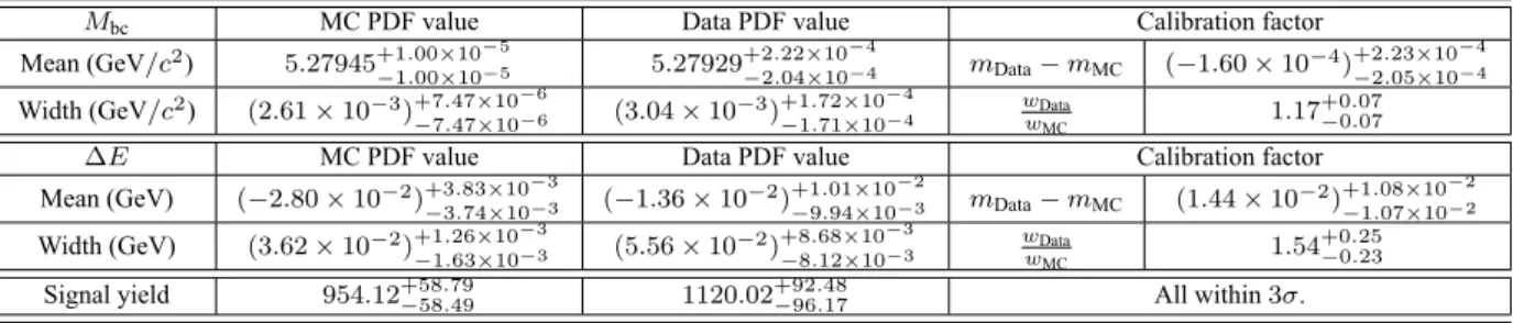
6.2.4 Calibration on PDF Shape . . . 66
6.2.5 Conclusion . . . 66
6.3 B0 → J/ψK0 . . . 67
6.3.1 Event Selection . . . 67
6.3.2 Background Suppression . . . 67
6.3.3 PDF Modeling and Fitting . . . 68
6.3.4 Calibration on Background Suppression Efficiency . . . 68
6.3.5 Conclusion . . . 70
7 Systematic Error Study 71 7.1 Tracking Uncertainty . . . 71
7.2 Number of B ¯B Pairs Uncertainty . . . . 71
7.3 Secondary Sub-decay Uncertainty . . . 71
7.4 Charged Particle Identification Uncertainty . . . 72
7.5 γ Identification Uncertainty . . . . 72
7.6 Background Suppression Uncertainty . . . 73
7.7 π0 Veto Uncertainty . . . 73
7.8 X(3872)→ J/ψρ0generation model . . . 73
7.9 Uncertainties Only for Fitting Method . . . 74
7.10 Uncertainties Only for Counting method . . . 75
7.11 Summary of Systematic Errors . . . 75
7.12 Summary for Calibration Factor . . . 75
8 Upper Limit Estimation 76 8.1 Counting Method . . . 76
8.1.1 Calibration on Signal Box Efficiency . . . 76
8.1.2 Expected Background in Signal Region . . . 77
8.1.3 Expected Counting Results . . . 78
8.2 Fitting Method . . . 78
8.2.1 Uncertainty on PDF Modeling . . . 79
8.2.2 Fitting bias . . . 79
8.2.3 Expected Fitting Results . . . 80
8.3 Dicision to use counting or fitting method . . . 80
9 Open Box Result 82 9.1 Counting Results . . . 82
9.2 Fitting Results . . . 83
10 Conclusion 85 A Plots of Event Selections 86 B Plots of Variables for NeuroBayes Training 87 B.1 B0 → X(3872)γ . . . 87
B.2 B0 → KS0π+π−γ . . . . 90
B.3 B0 → J/ψK0 . . . 92
C Fitting Plots for Control Samples 95 C.1 B0 → KS0π+π−γ . . . . 95
C.2 B0 → J/ψK0 . . . 98
C.2.1 Dimuon channel . . . 98
C.2.2 Dielectron channel . . . 98
D Scattering Plots 102 D.1 B0 → X(3872)γ . . . 102
D.2 B0 → KS0π+π−γ . . . 104
D.3 B0 → J/ψK0 . . . 105
E Pull and NsigDistributions for Signal Ensemble Tests 107 F Fitter Testing for Control Samples 110 F.1 B0 → KS0π+π−γ . . . 110
F.1.1 ToyMC ensemble test . . . 110
F.1.2 Gsim ensemble test . . . 111
F.2 B0 → J/ψK0 . . . 112
F.2.1 ToyMC ensemble test . . . 112
F.2.2 Gsim ensemble test . . . 112
Bibliography 114
Thesis Results Presented 121
List of Figures
1.1 Elementary particles in the Standard Model . . . 2
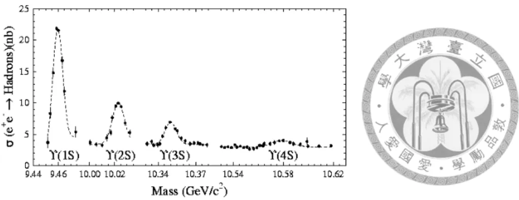
1.2 Total e+e−cross section measured by CLEO and CUSB showing the masses of Υ resonances. . . 3
1.3 e+e−→ Υ(4S) → B ¯B process . . . 3
1.4 Feynman diagrams for charmonium production at e+e−colliders. . . 5
1.5 Decay of charmonium states. . . 6
1.6 Spectrum for experimentally established charmonium(-like) states. . . 7
1.7 The discovery of X(3872) state by Belle experiment. . . . 9
1.8 A Feynman diagram of B0 → c¯cγ. . . 11
2.1 Aerial view of KEK and KEKB accelerator (May 2009) . . . 13
2.2 Illustration of beam bunches rotation by crab cavity . . . 13
2.3 Configuration of the KEKB accelerator . . . 14
2.4 Configuration of the Belle detector . . . 17
2.5 Configuration of the beam pipe . . . 19
2.6 Configuration of the SVD . . . 20
2.7 Graphical illustration of sub-detector SVD1 and SVD2 . . . 21
2.8 BGO crystals arrangement in forward and backward EFC detectors . . . . 22
2.9 Overview of the CDC structure . . . 23
2.10 Cell structure and the cathode sector configuration of the CDC . . . 23
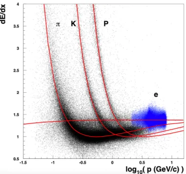
2.11 Scatter plot of dE/dx versus momentum . . . . 24
2.12 Arrangement of the central ACC in the Belle detector . . . 25
2.13 Schematic drawing of a typical ACC module . . . 25
2.14 Overview of a TOF/TSC module . . . 27
2.15 Mass distribution from TOF measurements for particle momenta below 1.2 GeV/c . . . . 27
2.16 ECL Overview . . . 29
2.17 Schematic drawings of the RPC internal arrangement . . . 30
2.18 Overview of the Solenoid Magnet and the Coil . . . 32
2.19 Overview of the hardware trigger system . . . 33
2.20 Overview of the DAQ system . . . 34
3.1 Distribution of P (π0) for signal and background MCs. . . 37
3.2 Bremsstrahlung photons coming from electrons. . . 38
3.3 Selections on Mππ. . . 39
3.4 Selections on ∆M . . . . 40
3.5 Typical & modified Mbc. . . 41
3.6 ∆E vs. typical/modified Mbc for dimuon channel. . . 41
3.7 ∆E vs. typical/modified Mbc for dielectron channel. . . 42
4.1 Two main types of background events. . . 43
4.2 Normalized outputs ofNeuroBayes training. . . 44
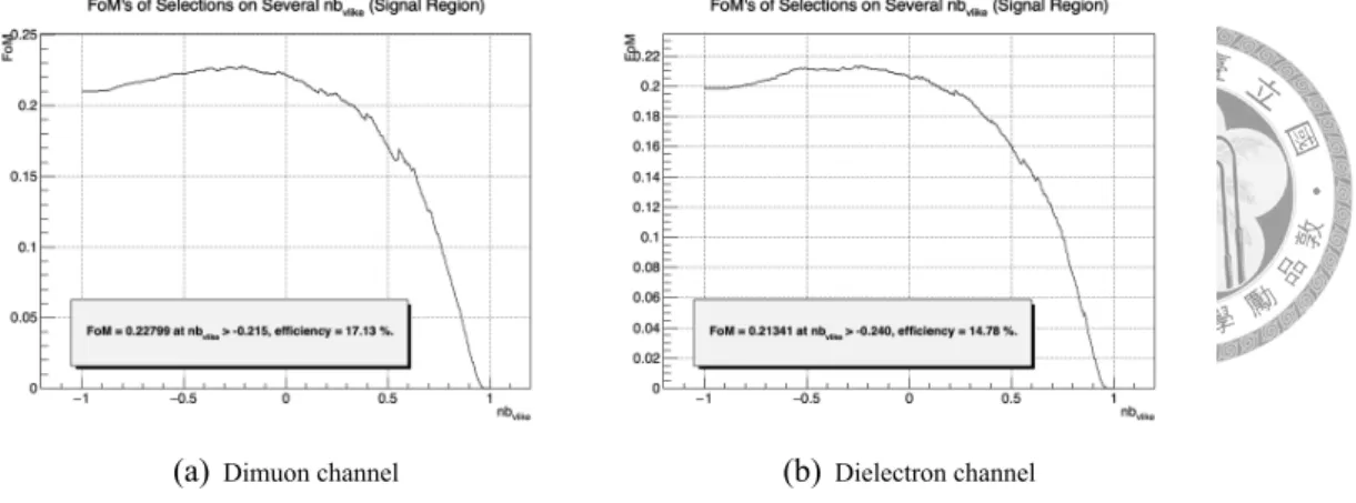
4.3 FOMs when applied on different values of background suppression cut. . 49
4.4 Multiplicity per event . . . 50
4.5 Mbcand ∆E after background suppression and BC selection. . . . 51
5.1 PDF for Mbc and ∆E in true signal for dimuon channel. . . . 55
5.2 PDF for Mbc and ∆E in B → J/ψX background for dimuon channel. . . 55
5.3 PDF for Mbc and ∆E in true signal for dielectron channel. . . . 56
5.4 PDF for Mbc and ∆E in B → J/ψX background for dielectron channel. 56 5.5 ToyMC ensemble test for dimuon channel . . . 57
5.6 Gsim ensemble test for dimuon channel . . . 58
5.7 ToyMC ensemble test for dielectron channel . . . 58
5.8 Gsim ensemble test for dielectron channel . . . 59
6.1 Training result and maximization on FOM. . . 64
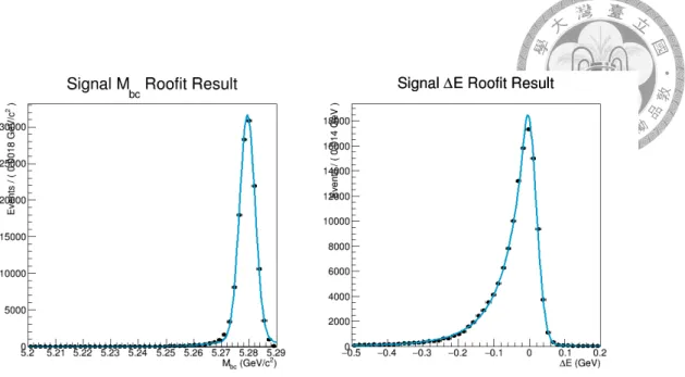
6.2 PDF for Mbc and ∆E in true signal. . . . 65
6.3 PDF for Mbc and ∆E in q ¯q background. . . . 65
6.4 PDF for Mbc and ∆E in true signal for dimuon channel. . . . 68
6.5 PDF for Mbc and ∆E in true signal for dielectron channel. . . . 69
7.1 Helicity angular distribution for different models. . . 74
8.1 Background MC and sideband data histogram . . . 77
8.2 Noutsigdistribution for Gsim ensemble test when generated Nsig = 0. . . 79
8.3 Likelihood function . . . 80
9.1 Two dimensional (Mbc,∆E) distributions of the selected B0 → X(3872)γ candidates. . . 82
9.2 Likelihood function . . . 83
9.3 Mbcand ∆E distributions of the selected B0 → X(3872)γ candidates. . . 84
A.1 Plots of event selections for signal MC. . . 86
B.1 Variables for NeuroBayes training for dimuon channel . . . 88
B.2 Variables for NeuroBayes training for dielectron channel . . . 89
B.3 Variables for NeuroBayes training for B0 → KS0π+π−γ (1) . . . . 90
B.4 Variables for NeuroBayes training for B0 → KS0π+π−γ (2) . . . . 91
B.5 Variables for NeuroBayes training for B0 → J/ψ(→ µ+µ−)K0 . . . 93
B.6 Variables for NeuroBayes training for B0 → J/ψ(→ e+e−)K0 . . . 94
C.1 Fitting for Mbc and ∆E with PDF width modification . . . . 96
C.2 Fitting for Mbc and ∆E without PDF width modification . . . . 97
C.3 Fitting for Mbc and ∆E of the dimuon channel before background sup- pression . . . 98
C.4 Fitting for Mbcand ∆E of the dimuon channel after background suppression 99 C.5 Fitting for Mbcand ∆E of the dielectron channel before background sup- pression . . . 100
C.6 Fitting for Mbc and ∆E of the dielectron channel after background sup-
pression . . . 101
D.1 Mbcvs. ∆E scattering plots for true signal MC . . . 102
D.2 Mbcvs. ∆E scattering plots for B → J/ψX MC . . . 102
D.3 Mbcvs. ∆E scattering plots for B ¯B background MC without J /ψ . . . . 103
D.4 Mbcvs. ∆E scattering plots for q ¯q background MC . . . 103
D.5 Mbcvs. ∆E scattering plots for true signal MC . . . 104
D.6 Mbcvs. ∆E scattering plots for B ¯B and rare decay background . . . 104
D.7 Mbcvs. ∆E scattering plots for true signal MC . . . 105
D.8 Mbcvs. ∆E scattering plots for B → J/ψX MC . . . 105
D.9 Mbcvs. ∆E scattering plots for B ¯B background MC without J /ψ . . . . 106
D.10 Mbcvs. ∆E scattering plots for q ¯q background MC . . . 106
E.1 Pull distributions of ToyMC ensemble test for dimuon channel . . . 107
E.2 Nsigdistributions of ToyMC ensemble test for dimuon channel . . . 107
E.3 Pull distributions of Gsim ensemble test for dimuon channel . . . 108
E.4 Nsigdistributions of Gsim ensemble test for dimuon channel . . . 108
E.5 Pull distributions of ToyMC ensemble test for dielectron channel . . . 108
E.6 Nsigdistributions of ToyMC ensemble test for dielectron channel . . . 109
E.7 Pull distributions of Gsim ensemble test for dielectron channel . . . 109
E.8 Nsigdistributions of Gsim ensemble test for dielectron channel . . . 109
F.1 Pull distribution of ToyMC test . . . 110
F.2 Pull distribution of Gsim test . . . 111
F.3 Pull distribution of Gsim test . . . 111
F.4 Pull distribution of ToyMC test . . . 112
F.5 Pull distribution of Gsim test (10,000 times, 1× Nsig) . . . 113
F.6 Pull distribution of Gsim test (10,000 times, 0.1× Nsig) . . . 113
F.7 Pull distribution of Gsim test (10,000 times, 0.01× Nsig) . . . 113
List of Tables
1.1 Properties of the four types of B mesons. . . . 3
2.1 Parameters of the KEKB accelerator design. . . 15
2.2 Performance parameters for the Belle detector. . . 18
2.3 Geometrical parameters of ECL in each region . . . 28
2.4 Trigger rate for each process at the designed operation luminosity. . . 32
3.1 EvtGen models used for signal MC samples. . . 36
3.2 Types of background MC samples used. . . 36
3.3 Summary of basic selection criteria. . . 42
4.1 The M M2regions. . . 46
4.2 Summary ofNeuroBayes input parameters. . . 48
4.3 Background suppression cut with best FOM. . . 49
4.4 Signal efficiency & background number before/afterNeuroBayes & Best Candidate selection. . . 52
5.1 Linear correlation factor between ∆E and Mbc. . . 54
5.2 PDFs for fitter of dimuon channel. . . 54
5.3 PDFs for fitter of dielectron channel. . . 55
5.4 Float variables in 2D fitting. . . 55
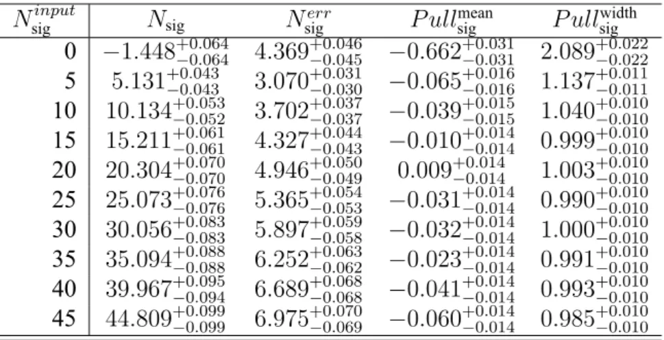
5.5 ToyMC ensemble test detailed result for dimuon channel . . . 60
5.6 Gsim ensemble test detailed result for dimuon channel . . . 60
5.7 ToyMC ensemble test detailed result for dielectron channel . . . 61
5.8 Gsim ensemble test detailed result for dielectron channel . . . 61
6.1 EvtGen models used for B0 → KS0π+π−γ signal MC samples. . . . 62
6.2 Basic selection criteria for B0 → KS0π+π−γ . . . . 63
6.3 NeuroBayes input parameters for B0 → KS0π+π−γ. . . . 63
6.4 qq suppression cut with best FOM. . . . 64
6.5 PDFs for fitter of B0 → KS0π+π−γ . . . . 64
6.6 Calibration on mean and width shift for signal PDF . . . 66
6.7 Summary of the control sample B0 → KS0π+π−γ. . . . 66
6.8 EvtGen models used for B0 → J/ψK0signal MC samples. . . 67
6.9 Basic selection criteria for B0 → J/ψK0 . . . 67
6.10 PDFs for fitter of B0 → J/ψK0 . . . 68
6.11 Calibration on background suppression efficiency . . . 69
6.12 Summary of the control sample B0 → J/ψK0. . . 70
7.1 Calibration factor and uncertainty on charged particle identification. . . . 72
7.2 Helicity angular distribution for different models. . . 74
7.3 Signal efficiency with the corresponding error for different models . . . . 74
7.4 Systematic errors of signal efficiency. . . 75
7.5 Calibration factors on signal efficiency. . . 75
8.1 Systematic error on background level . . . 77
8.2 Expected Counting Results . . . 78
8.3 Expected Fitting Results . . . 80
8.4 Compare the upper limits obtained by the two methods . . . 81
9.1 Counting Results from data . . . 83
9.2 Data Fitting Results . . . 83
9.3 Fitting yields for signal and background. . . 84
Chapter 1 Introduction
1.1 Standard Model
The Standard Model (SM) is a quantum field theory that describes the properties of el- ementary particles as well as their interactions. Until now, basically most experimental results of particle physics can be explained by SM. In the SM, elementary particles can be classified into four categories: quarks, leptons, gauge bosons, and Higgs boson. The interactions described in SM includes electromagnetic, weak, and strong interaction.
Both quarks and leptons are spin-12 fermions with three generations and six types.
Quarks carry fractional charge (±13 or±23) while leptons carry integer charge (±1 or 0).
Gauge bosons are spin-1 force-carriers: Photon carries the electromagnetic force, gluons carry the strong force, while W±and Z bosons carry weak force. Higgs boson, the last dis- covered elementary particle in the SM, is spin-0 and can explain the origin of elementary particles’ mass. All the particles in SM can experience weak interaction; particles with electric charges can experience electromagnetic interaction; particles with color charge (quarks and gluons) can experience strong interaction.
There are three types of color charge: r, g, and b, and each quark carries one type of color. The color confinement principle in QCD makes it impossible to observe a single quark: the quarks can only be observed as a stable form of hadrons including baryons (qqq) or meson (q ¯q), which is colorless and has integer electric charges. The properties of all elementary particles in the SM are summarized in Fig. 1.1(a), and the interactions
among them are shown in Fig. 1.1(b).
(a) Properties of elementary particles. [1] (b) Interactions among elementary particles. [2]
Figure 1.1: Elementary particles in the Standard Model
1.2 B Physics
The physics related to the B mesons can be abbreviated as “B physics”. B mesons com- posed of a bottom quark (b) and another light quark (u, d, s, or c, each has its corresponding type of B mesons: B±, B0, Bs0, and Bc±). Their properties are shown in Table. 1.1.
The b-quark was observed in 1977 by the Columbia-Fermilab-Stony Brook collabo- ration (CFS) E288 experiment [3] in the newly discovered di-muon resonance, which is now recognized as Υ(1S). Later, the B mesons were found by the CLEO experiment in Cornell Electron Storage Ring (CESR) at Cornell University, in the decays of the excited resonance state Υ(4S). Fig. 1.2 shows the cross section of different Υ states measured by CLEO and CUSB (Columbia University - Stony Brook). [4]
Since the mass of Υ(4S) is (10579.4± 1.2) MeV, which is only 20 MeV above the B ¯B threshold, and the branching fractionB(Υ(4S) → B ¯B) > 96% [6], B mesons can be produced in abundance from the decay of Υ(4S). Experimentally, we produce B mesons by e+e− collisions at a center-of-mass energy on the Υ(4S) resonance, and the Υ(4S) almost immediately decays to either B+B− or B0B¯0 pairs, and their branching fractions are almost the same. The Feynman diagram for such process is shown in Fig. 1.3. Such
Figure 1.2: Total e+e−cross section measured by CLEO and CUSB showing the masses of Υ resonances. [5]
kind of experimental design dedicated to the Υ(4S) production is called B-factory, which is essential for the study of B physics, including rare B decays and CP violation in the B decay. The majority of B decays via b → c transition, with a charmed hadron or charmonium (c¯c mesons) in the final state. Rare B decay is a powerful probe for the physics beyond SM. The Belle experiment in KEKB accelerator of KEK and the BaBar experiment in PRP-II accelerator of SLAC are the two B-factories in the world.
Type Quark content I(JP) Rest mass (MeV/c2) Mean lifetime (ps) B± ¯bu 12(0−) 5279.32± 0.14 1.638± 0.004 B0 ¯bd 12(0−) 5279.63± 0.15 1.520± 0.006 Bs0 ¯bs 0(0−) 5366.89± 0.19 1.527± 0.011 Bc± ¯bc 0(0−) 6274.9± 0.8 0.507± 0.009
Table 1.1: Properties of the four types of B mesons. [6]
Figure 1.3: e+e−→ Υ(4S) → B ¯B process
1.3 Charmonium and the X(3872) State
1.3.1 Charmonium States
Charmonium states are flavorless mesons composed of a charm quark (c) and an anti- charm quark (¯c), and they have masses around 3 GeV/c2. The first charmonium state J /ψ was found in November 1974 independently by two experimental groups at SLAC and Brookhaven [7, 8], and its excited state ψ(2S) (which was called ψ′ at that time) was also found by the SLAC group later [9]. The discoveries confirmed the existence of the charm quark and its antiquark which had been predicted several years before [10]. Since then, the charmonium state has been used as a powerful tool to understand the strong interactions.
There are many ways to produce charmonium states at e+e− colliders, including di- rect production from e+e− annihilation (e.g. e+e− → ψ(2S) → χc0(1P )γ), B-meson decay (e.g. B+ → X(3872)K+), initial state radiation (e.g. e+e− → γISRY (4260)), two virtual photon production (photon-photon fusion, e.g. γγ → ηc(2S)), and double charmonium production (e.g. e+e− → J/ψηc). Their corresponding Feynman diagrams are shown in Fig. 1.4. The charmonium states decays via several different process, in- cluding annihilation (e.g. J /ψ → µ+µ−), strong decay (e.g. J /ψ → ggg → hadrons, J /ψ → γgg → hadrons, and ψ(2S) → J/ψπ+π−), electromagnetic (radiative) decay (e.g. X(3872)→ J/ψγ), and weak decay (e.g. J/ψ → D−se+νeand J /ψ → ¯D0e+e−).
Their corresponding Feynman diagrams are shown in Fig. 1.5.
Since the c¯c state is a two-body system analogous to a hydrogen atom, it can be de- scribed with the same quantum numbers as that of a hydrogen atom: n, L, S and J , which are the radial quantum number, orbital quantum number, total spin, and total angular mo- mentum, respectively. Charmonium spectroscopy is ideal for studying the QCD dynam- ics between the perturbative and non-perturbative QCD regime. The charmonium spec- trum for experimentally established charmonium and charmonium-like states is shown in Fig. 1.6 with the JP C values of each states. The nomenclature for charmonium states are defined by the following rules: states with even J and P C = −+ are named ηc(nL);
states with odd J and P C = +− are named hc(nL); states with P C = ++ are named
doi:10.6342/NTU201901047
χcJ(nL); states with P C =−− are named ψ(nL) except J/ψ for historical reasons. All predicted charmonium states below the D ¯D threshold have been observed.
e
e
+c ¯
c
b
c c
s
q q
W
e e
c c
e
+e
+e
e
+c ¯
c
e
e
+c ¯
c c
c
c
¯
c e
+e
(a) e+e−annihilation
e
e
+c ¯
c
b
c c
s
q q
W
e e
c c
e
+e
+e
e
+c ¯
c
e
e
+c ¯
c c
c
c
¯
c e
+e
1
(b) B-meson decay
e
e
+¯ c
c
b
c c
s
q q
W
e e
c c
e
+e
+e
e
+¯ c
c
e
e
+¯ c
c c
c
c
¯
c e
+e
1
(c) Initial state radiation
e
e
+c ¯
c
b
c c
s
q q
W
e e
c c
e
+e
+e
e
+c ¯
c
e
e
+c ¯
c c
c
c
¯
c e
+e
1
(d) Photon-photon fusion
e
e
+¯ c
c
b
c c
s
q q
W
e e
c c
e
+e
+e
e
+¯ c
c
e
e
+¯ c
c c
c
c
¯
c e
+e
1
(e) Double charmonium production
Figure 1.4: Feynman diagrams for charmonium production at e+e−colliders.
5
doi:10.6342/NTU201901047
e
e
+c ¯
c
b
c c
s
q q
W
e e
c c
e
+e
+e
e
+c ¯
c
e
e
+c ¯
c c
c
c
¯
c e
+e
1
(a)
c c
c
c d
d
c
¯
c u ¯
u d ¯ d d ¯ d
c c
c c d u
u d
c c
c c
c c
s, d c
⌫
ee
+W
+c u
c c
, Z W
+b
2
(b)
c c
c
c d
d
c
¯
c u¯
u d¯ d d¯ d
c c
c c d u
ud
c c
c c
c c
s, d c
⌫e e+ W+
c u
c c
, Z W+
b
(c)
c
c
c
c d
d
c
¯
c u ¯
u d ¯ d d ¯ d
c c
c c d u
u d
c c
c c
c c
s, d c
⌫
ee
+W
+c u
c c
, Z W
+b
2
(d)
c c
c
c d
d
c
¯
c u ¯
u d ¯ d d ¯ d
c c
c c d u
u d
c c
c c
c c
s, d c
⌫ e e + W +
c u
c c
, Z W +
b
2
(e)
c c
c
c d
d
c
¯
c u ¯
u d ¯ d d ¯ d
c c
c c d u
u d
c c
c c
c c
s, d c
⌫
ee
+W
+c u
c c
, Z W
+b
2
(f)
c
c
c
c d
d
c
¯
c u ¯
u d ¯ d d ¯ d
c c
c c d u
d u
c c
c c
c c
s, d c
⌫
ee
+W
+c u
c c
, Z W
+b
2
(g)
Figure 1.5: Decay of charmonium states. (a) Annihilation, (b-d) strong decay, (e) radiative decay, (f,g) weak decay.
6
c(1S) η
c(2S) η
ψ J/
ψ(2S) (3770) ψ
(4040) ψ
(4160) ψ Y(4260) Y(4360) (4415) ψ Y(4660)
c(1P) h
c0(1P) χ
c1(1P) χ X(3872)
c2(1P) χ
c2(2P) χ
D D
* D D
Ds
Ds
* D D*
* D
s* D
s* D
s* D Thresholds:
−+
0 1−− 1+− 0++ 1++ 2++
JPC
3000 3200 3400 3600 3800 4000 4200 4400 4600 ]2 Mass [MeV/c
Figure 1.6: Spectrum for experimentally established charmonium(-like) states. [6]
1.3.2 Charmonium-like Exotic States
Since the discovery of the X(3872) state in 2003, there are more and more newly-found charmonium-like states which do not seem to have a pure c¯c structure. Instead, they have some exotic properties indicating that they may be candidates of tetraquark or hybrid states. These states are also called XYZ states experimentally. Their masses and decay channels do not agree with the predictions of pure charmonium models.
Tetraquark states are colorless combination of four quarks. There are three types of tetraquark states: meson molecule, compact tetraquark state, and hadro-charmonium. Me- son molecules comprised of two charmed mesons loosely bound together, and their bind- ing mechanisms including quark exchange at short distances and pion exchange at longer distances. The pion exchange mechanism is expected to be dominant [11]. Compact tetraquark state is described as a diquark-diantiquark structure (diquarkonia) in the model of Maiani et al. [12], where the quarks are grouped into color-triplet scalar and vector clusters. A simple spin-spin interaction is dominant, and the strong decays are expected to
proceed through rearrangement processes followed by dissociation. Hadro-charmonium state consists of a compact c¯c core surrounded by a cloud of light hadronic matter with a typical radius much larger. The hadrocharmonium candidates (e.g. Zc(4430)) decay pre- dominantly to a particular charmonium and light mesons, and are not observed decaying into open charm final states [13]. The possible existence of multiplets that include mem- bers with nonzero charge and/or strangeness may distinguishes tetraquark states from the conventional charmonia.
The charmonium hybrid state (c¯cg) consist of a color-octet quark-antiquark pair and an excited gluon. Since hybrids have additional gluonic degrees of freedom, they are able to have exotic quantum numbers (e.g. JP C = 0−−, 0+−, 1−+, 2+− etc.) which are inaccessible for pure charmonia. Heavy quarkonium hybrids have been studied by sev- eral different models and calculational schemes, including lattice QCD [14, 15], the flux tube model [16], the constituent gluon model [17], and the quasi-gluon model [18]. A lattice QCD model [14, 15] describes the quarks as moving in gluon-produced adiabatic potentials, which is analogous to the molecules where atomic nuclei are moving in the electron-produced adiabatic potentials. Lattice QCD and most models predict that the lowest mass for a charmonium hybrid state should be roughly 4.4 GeV/c2.
1.3.3 The X(3872) State
The X(3872) state was first observed by Belle experiment in 2003 as a peak in the J /ψπ+π− invariant mass spectrum in the exclusive B+ → K+π+π−J /ψ decays (Fig. 1.7) [19].
Later on, this state was also observed in the high-energy proton-antiproton (p¯p) collisions by Collider Detector at Fermilab (CDF) [20] and DØ [21] collaboration at the Fermilab Tevatron, as well as in the B meson decays by BaBar collaboration. Currently, its world average mass is (3871.69± 0.17) MeV/c2, and its total width is less than 1.2 MeV/c2 [6].
X(3872) is now one of the most famous charmonium-like exotic states.
The observation of the decay X(3872) → J/ψγ by both Belle [22] and BaBar [23]
experiments shows that the charge parity is C = +1, and this assignment is further sup- ported by the π+π−invariant mass spectrum in X(3872) → J/ψπ+π− decays analyzed
doi:10.6342/NTU201901047
signal. To determine an upper limit on the total width, we repeated the fits using a resolution-broadened Breit- Wigner (BW) function to represent the signal. This fit gives a BW width parameter that is consistent with zero:
! ! 1:4 " 0:7 MeV. From this we infer a 90% confidence level (C.L.) upper limit of ! < 2:3 MeV.
The open histogram in Fig. 3(a) shows the !
#!
$invariant mass distribution for events in a "5 MeV win- dow around the X%3872& peak; the shaded histogram shows the corresponding distribution for events in the nonsignal "E-M
bcregion, normalized to the signal area. The !
#!
$invariant masses tend to cluster near the kinematic boundary, which is around the " mass; the entries below the " are consistent with background. For comparison, we show the !
#!
$mass distribution for the
0
events in Fig. 3(b), where the horizontal scale is shifted and expanded to account for the different kinematically allowed region. This distribution also peaks near the upper kinematic limit, which in this case is near 590 MeV.
We determine a ratio of product branching fractions for B
#! K
#X%3872&, X%3872& ! !
#!
$J= and B
#! K
# 0,
0! !
#!
$J= to be
B!B
#! K
#X%3872&" ' B!X%3872& ! !
#!
$J= "
B%B
#! K
# 0& ' B%
0! !
#!
$J= & ! 0:063 " 0:012%stat& " 0:007%syst&:
Here the systematic error is mainly due to the uncertain- ties in the efficiency for the X%3872& ! !
#!
$J= chan- nel, which is estimated with MC simulations that use different models for the decay [13].
The decay of the
3D
c2charmonium state to #$
c1is an allowed E1 transition with a partial width that is ex- pected to be substantially larger than that for the
!
#!
$J= final state; e.g., the authors of Ref. [4] pre- dict !%
3D
c2! #$
c1& > 5 ' !%
3D
c2! !
#!
$J= &. We searched for an X%3872& signal in the #$
c1decay chan- nel, concentrating on the $
c1! #J= final state.
We select events with the same J= ! ‘
#‘
$and charged kaon requirements plus two photons, each with energy more than 40 MeV. We reject photons that form a
!
0when combined with any other photon in the event. We require one of the #J= combinations to satisfy
398 MeV < %M
#‘#‘$$ M
‘#‘$& < 423 MeV (correspond- ing to $15 MeV < %M
#J=$ M
$c1& < 10 MeV). In the following we use M
#$c1( M
##‘#‘$$ M
#‘#‘$# M
PDG$c1, where M
PDG$c1is the PDG $
c1mass value [9].
The B ! K#$
c1, $
c1! #J= decay processes have a large combinatoric background from B ! K$
c1decays plus an uncorrelated # from the accompanying B meson.
This background produces a peaking at positive "E val- ues that is well separated from zero and is removed by the
"E < 30 MeV requirement. Because of the complicated
"E background shape and its correlation with M
bc, we do not include "E in the likelihood fit. Instead, we perform an unbinned fit to the M
#$c1and M
bcdistributions with the same signal and background PDFs for M
bcand M
#$c1that are used for the !
#!
$J= fits. We fix the Gaussian widths at their MC values, and the
0and X%3872& masses at the values found from the fits to the !
#!
$J= chan- nels. The signal yields and background parameters are allowed to float.
The signal-band projections of M
bcand M
#$c1for the
0
region are shown in Figs. 4(a) and 4(b), respectively, together with curves that show the results of the fit. The fitted signal yield is 34:1 " 6:9 " 4:1 events, where the first error is statistical and the second is a systematic error determined by varying the M
bcand M
#$c1resolutions over their allowed range of values. The number of ob- served events is consistent with the expected yield of 26 " 4 events based on the known B ! K
0and
0!
#$
c1branching fractions [9] and the MC-determined acceptance.
The results of the application of the same procedure to the X%3872& mass region are shown in Figs. 4(c) and 4(d). Here, no signal is evident; the fitted signal yield is
0.400 0.50 0.60 0.70 0.80
2.5 5
Events/0.008 GeV
0.31 0.41 0.51 0.61
M(π+π-) (GeV)
0 12.5 25
Events/0.006 GeV
FIG. 3. M%!
#!
$& distribution for events in the (a) M%!
#!
$J= & ! 3872 MeV signal region, and (b) the
0region. The shaded histograms are sideband data normalized to the signal-box area. Note the different horizontal scales.
(GeV) Mbc
5.2 5.22 5.24 5.26 5.28 5.3
Events / ( 0.005 GeV )
0 5 10 15 20 25 30 35 40 a)
) (GeV) π π ψ
3.82 3.84 3.86 3.88 3.9 3.92M(J/
Events / ( 0.005 GeV )
0 5 10 15 20 25 30 35 b)
E (GeV)
-0.1 -0.05 0 0.05 0.1 0.15 0.2∆
Events / ( 0.015 GeV )
0 5 10 15 20 25 c)
FIG. 2 (color online). Signal-band projections of (a) M
bc, (b) M
!#!$J=, and (c) "E for the X%3872& ! !
#!
$J= signal region with the results of the unbinned fit superimposed.
P H Y S I C A L R E V I E W L E T T E R S week ending 31 DECEMBER 2003
V OLUME 91, N UMBER 26
Figure 1.7: The discovery of X(3872) state by Belle experiment. Figure shows the signal- band projections on (a) Mbc, (b) MJ /ψππ, and (c) ∆E for the X(3872)→ π+π−J /ψ signal region with the results of the unbinned fit superimposed. [19]
by both Belle [24] and CDF [25] experiments, which shows that the dipion system origi- nates from ρ0 → π+π− decay. Since ρ0 carries isospin I = 1 and a pure c¯c state carries I = 0, such process would violate isospin if we consider X(3872) as a pure charmonium state. Possible mechanisms to induce the isospin violation including the u/d quark mass difference in strong interaction and u/d quark charge difference in electromagnetic inter- actions. Also, the evidence for the isospin conserved mode X(3872)→ π+π−π0J /ψ by Belle [22] and BaBar [26] has a comparative branching fraction to X(3872)→ J/ψπ+π−, which implies that the X(3872) is a mixture of both I = 0 and I = 1 as suggested by Close and Page [27]. Furthermore, the angular correlations among the final-state particles from X(3872) → J/ψπ+π− decays has shown that JP C = 1++ or 2−+ for X(3872) [28]. In 2013, the 2−+ hypothesis was ruled out by LHCb with 8.2σ by five- dimensional angular correlations of B+ → X(3872)K+, where X(3872) → J/ψπ+π− and J /ψ → µ+µ−[29]. However, it does not fit the mass of the predicted pure charmo- nium state χc1(23P1) with JP C = 1++which was expected to be about 3953 MeV [30].
Also, the absence of a strong χcJγ [31] decay is inconsistent with the pure charmonium model.
Since X(3872) lies within 200 keV of the D0D¯∗0threshold, it is natural to interpret it as a D ¯D∗ molecule [32, 33]. The comparable branching fractions for X(3872)→ J/ψω and X(3872)→ J/ψρ0are consistent with this model as we consider the different widths of the ρ and ω [34]. A molecule-charmonium mixture scenario is also probable [35].
9
Another possible interpretation for X(3872) is the compact tetraquark cq¯c¯q state [12].
Although such interpretation becomes unlikely since its charged partner X(3872)+has not been found [36], there are still some possible explanation for its absence in the compact tetraquark scenario [37]. The LHCb measurement on the branching fraction of the decay X(3872)→ ψ(2S)γ compared to that of the decay X(3872) → J/ψγ does not support the interpretation of a pure D ¯D∗ molecule, while it agrees with the predictions of a pure charmonium state or a mixture of a molecule and a charmonium [38]. Other interpretations of X(3872) including the hybrid meson (c¯cg) [27, 39] as well as the vector glueball [40].
However, the former one is unlikely since the lowest mass for a charmonium hybrid state should be roughly 4.4 GeV/c2 predicted by lattice QCD calculations [41], and the latter one was also disproved by the observation of the X(3872)→ J/ψγ decay.
1.4 Motivation
Rare decays of B mesons are sensitive probes to study possible new physics beyond the SM. In the SM, the decay B0 → c¯cγ proceeds dominantly through an exchange of a W - boson and the radiation of a photon from the d quark of the B meson (Fig. 1.8). Many the- oretical predictions of branching fractions depend on the factorization approach of QCD interactions in the decay dynamics. In the case of B0 → J/ψγ, the branching fraction has been predicted to be 7.65× 10⁻⁹ using QCD factorization [42] and 4.5× 10⁻⁷ when using a perturbative QCD (pQCD) approach [43]. Possible new physics enhancements of the branching fractions may be due to right-handed currents [42] or non-spectator intrinsic charm in the B0meson [44]. Currently, the upper limit for B0 → J/ψγ is 1.5 × 10⁻⁶at 90% confidence level [45].
The exotic X(3872) state, first observed by the Belle experiment in 2003 in the exclu- sive B+ → K+X(3872)(→ π+π−J /ψ) decay [19], is now one of the most well-studied charmonium-like exotic states. Aside from pure charmonium, it may also be a D0D¯∗0 molecule [33], a tetraquark state [12], or a mixture of a molecule and a charmonium [35].
Since X(3872) may, unlike the J /ψ, contain components other than pure charmonium, the branching fraction of B0 → X(3872)γ should be smaller than that of B0 → J/ψγ
which proceeds through the b → c¯c d process. No former experimental result for this decay mode has been published yet.
Figure 1.8: A Feynman diagram of B0 → c¯cγ.
Chapter 2
The Belle Experiment
The Belle experiment ran at the KEK B-factory (KEKB) e+e−asymmetric energy collider in the Tsukuba campus of High Energy Accelerator Research Organization (KEK), Japan between 1999 and 2010. It was conducted by the Belle Collaboration, an international collaboration where more than 400 physicists and engineers from 20 different countries participated in. Although the Belle experiment was designed and optimized for the study of CP violation in the B meson system, it also performed extensive studies on rare decays, exotic states, properties of D mesons and τ particles. Fig. 2.1 shows an aerial view of the KEKB accelerator.
2.1 KEKB Accelerator
The KEK B-factory (KEKB), served as the beam provider in the Belle experiment, was an asymmetric energy electron-positron collider with two storage rings: a low-energy ring (LER, for 3.5 GeV positron beam) and a high-energy ring (HER, for 8 GeV electron beam).
Both rings were constructed alongside in the TRISTAN tunnel with circumference of 3 km.
The two beams collided with a crossing angle of±11 mrad at the interaction point (IP) in Tsukuba hall, where the Belle detector located, on the northeast side of the rings. The collision energy was 10.58 GeV at the Υ(4S) resonance in the center-of-mass frame, just barely above the B ¯B production threshold. At this energy, the cross section of e+e− → Υ(4S) is about 1.05 nb, while the continuum process e+e− → q¯q (q ∈ {u, d, s, c}) is
Figure 2.1: Aerial view of KEK and KEKB accelerator (May 2009) [46]
about 3.7 nb.
The design of finite crossing angle between the two beams can enhance the luminosity by reducing the parasitic collisions near IP. This also eliminated the needs of separation- bend magnets, and thus significantly reduced the beam backgrounds in the detector. Fur- thermore, such design let us be able to fill all RF buckets with the beam. Crab cavities are also placed near the IP to rotate the e+e− beam bunches just before the collision in order to make head-on collision, as shown in Fig. 2.2. The head-on collision maximizes the beam overlap at IP and therefore increase the luminosity further.
Figure 2.2: Illustration of beam bunches rotation by crab cavity [47]
There are other three straight sections in the circular tunnel: Fuji, Nikko and Oho. The beams from the Linac were injected to the rings in the Fuji area, where a cross-over design is used to ensure the circumference of the two rings were exactly the same. In Nikko and Oho areas, the RF cavity for HER is installed in the straight section, and the wigglers for LER are also reserved in the two areas. The configuration of KEKB accelerator is illustrated in Fig. 2.3, and the parameters for its design are summarized in Table. 2.1.
Figure 2.3: Configuration of the KEKB accelerator. [48]
The peak luminosity of KEKB exceeded 2.11× 1034cm−2s−1, and the total integrated luminosity of 1052 fb−1was recorded by the Belle detector. Both of them achieved world records at that time. KEKB has operated from 1998 to 2010. After that, the KEKB ac- celerator and the Belle detector are upgraded to SuperKEKB and Belle II, designed to increase the instantaneous luminosity by a factor of 40 [49]. The first physics data taking run for Belle II analyses has begun in March 2019 [50].
Ring LER HER Unit
Energy E 3.5 8.0 GeV
Beam current I 2.6 1.1 A
Circumference C 3016.26 m
Luminosity L 1× 1034 cm−2s−1
Crossing angle θx ±11 mrad
Tune shifts ξx/ξy 0.039/0.052
Energy spread σε 7.1× 10⁻⁴ 6.7× 10⁻⁴
Beta function at IP βx∗/βy∗ 0.33/0.01 m
Natural bunch length σz 0.4 cm
Bunch spacing sb 0.59 m
Particles/bunch N 3.3× 10¹⁰ 1.4× 10¹⁰
Emittance ε∗x/ε∗y 1.8× 10⁻⁸/3.6× 10−10
Synchrotron νs 0.01∼ 0.02
Betatron tune νx/νy 45.52/45.08 47.52/43.08 Momentum compaction factor αp 1× 10⁻⁴∼ 2 × 10⁻⁴
Energy loss/turn U0 0.81†/1.5†† 3.5 MeV
RF voltage Vc 5∼ 10 10∼ 20 MV
RF frequency fRF 508.887 MHz
Harmonic number h 5120
Longitudinal damping time τε 43†/23†† 23 ms
Total beam power Pb 2.7†/4.5†† 4.0 MW
Radiation power PSR 2.1†/4.0†† 3.8 MW
HOM power PHOM 0.57 0.15 MW
Bending radius ρ 16.3 104.3 m
Length of bending magnet lB 0.915 5.86 m
†: without wigglers, ††: with wigglers
Table 2.1: Parameters of the KEKB accelerator design. [51]
2.2 Belle Detector
The Belle detector was a multi-layer detector with various sub-detectors, configured with a 1.5T superconducting solenoid and iron structure surrounding the KEKB beams at the Tsukuba interaction region. The main structure of the detector extends from the polar angle (θ) 17◦to 150◦. The sub-detectors arranged like onion scales around from the IP to the outer layers, which were SVD, EFC, CDC, ACC, TOF, ECL, and KLM, respectively.
Brief introductions to them are below:
• Silicon Vertex Detector (SVD): The inner-most detector, consists of a silicon strip detector with four layers, which measures B decay vertices precisely.
• Extreme Forward Calorimeter (EFC): A pair of BGO crystal arrays, which detects tracks from the extreme forward and backward directions, to extend the polar angu- lar coverage of ECL.
• Central Drift Chamber (CDC): A cylindrical volume with 8400 wires distributed in 50 layers, located outside of beam pipe and SVD. It provides tracking, dE/dx and momentum information of charged particles.
• Aerogel Čerenkov Counters (ACC): An array of silica aerogel threshold Čerenkov counters, which provides particle identification information.
• Time of Flight (TOF): Barrel-like arranged time-of-flight scintillation counters, which measures the particle flight time for particle identification.
• Electromagnetic Calorimeter (ECL): A CsI(Tl) scintillator crystal array, which is located outside of ACC and TOF and inside the coil of solenoid magnet. It detects the position and energy of photons and also contributes to electron identification.
• KL0 and muon detection system (KLM): An iron magnetic flux-return located out- side the solenoid magnet coil, which identifies KL0 and muon.
![Figure 2.8: BGO crystals arrangement in forward and backward EFC detectors. [52]](https://thumb-ap.123doks.com/thumbv2/9libinfo/9608622.634144/40.892.256.638.304.700/figure-bgo-crystals-arrangement-forward-backward-efc-detectors.webp)
![Figure 2.10: Cell structure and the cathode sector configuration of the CDC. [52]](https://thumb-ap.123doks.com/thumbv2/9libinfo/9608622.634144/41.892.198.689.731.966/figure-cell-structure-cathode-sector-configuration-cdc.webp)

![Figure 2.14: Overview of a TOF/TSC module. The unit of length is in mm. [52]](https://thumb-ap.123doks.com/thumbv2/9libinfo/9608622.634144/45.892.162.785.91.365/figure-overview-tof-tsc-module-unit-length-mm.webp)