國
立
交
通
大
學
管理科學系
博
士
論
文
科技產品生命週期之預測模型比較
An Evaluation of Models for Forecasting Technology Product
Lifecycles
研 究 生:吳欣穎
指導教授:張力元 教授
國
立
交
通
大
學
管理科學系
博
士
論
文
科技產品生命週期之預測模型比較
An Evaluation of Models for Forecasting Technology Product
Lifecycles
研 究 生:吳欣穎
研究指導委員會:黃仁宏 教授
王耀德 教授
指導教授:張力元 教授
中 華 民 國 九 十 八 年 六 月
科技產品生命週期之預測模型比較
An Evaluation of Technology Forecasting Models for Forecasting Short Product
Lifecycles
研 究 生:吳欣穎 Student:Hsin-Ying Wu
指導教授:張力元 Advisor:Charles V. Trappey
國 立 交 通 大 學
管理科學系
博 士 論 文
A DissertationSubmitted to Department of Management Science College of Management
National Chiao Tung University in Partial Fulfillment of the Requirements
for the Degree of Doctor of Philosophy
in
Management
June 2009
Hsin-Chu, Taiwan, Republic of China
科技產品生命週期之預測模型比較
研究生:
吳欣穎指導教授
:張力元國立交通大學管理科學系博士班
中文摘要
成長曲線模型常常被使用來預測科技產品之走向與趨勢,本研究利用 22 組科技產 品資料來比較 The simple logistic model, the Gompertz model, and the time-varying extended logistic model,此三種科技預測模型之預測準確度,再歸納出此三種模型 之優缺點及建議使用時機。結果發現,The time-varying extended logistic model 對 在 70%的科技產品上,都有比 Simple logistic model 與 Gompertz model 兩個模型較 好的預測準確度;但由於 The time-varying extended logistic model 在模型設定時需 要有較多的參數來估計成長上限,在資料點太少的情況下,有約 20%的機率無法 得到收斂的結果,因此本研究建議若欲使用 Extended logistic model,最好有 15 點 以上之連續資料,且產品成長曲線有 S 曲線的軌跡,將會有較準確的預測結果。 本研究亦提出一個選擇預測模型的決策流程,建議若在 Extended logistic model 無 法收斂的情況下,但該產品成長曲線之反曲點已出現,則 Simple logistic model 與 Gompertz model 可被使用來預測產品未來的發展空間。本研究亦利用大陸 RFID 專 利申請案數量為一應用該決策流程之個案,並進一步預測未來 RFID 產業的發展趨 勢。最後,本研究也提出對產品生命週期各階段之策略建議。
關鍵詞:
科技預測、簡單羅吉斯模式、甘伯茲模式、廣泛羅吉斯模式、產品生An Evaluation of Models for Forecasting Technology Product Lifecycles
Student:Hsin-Ying Wu
Advisor:Dr. Charles Trappey
Department of Management Science
National Chiao Tung University
ABSTRACT
Many successful technology forecasting models have been developed but few researchers have explored a model that can best predict short product lifecycles. This research studies the forecast accuracy of long and short product lifecycle datasets using simple logistic, Gompertz, and the extended logistic models. Time series datasets for 22 electronic products were used to evaluate and compare the performance of the three models. The findings show that the time-varying extended logistic model fits short product lifecycle datasets 70% better than the simple logistic and the Gompertz models. A decision diagram is proposed to select a suitable forecasting model among the three models. The results suggest that there should be at less fifteen data points for the extended logistic model to reach better predictions. However, if the extended logistic model cannot be applied and the inflection point of the growth curve is revealed, the simple logistic and the Gompertz models can be the alternatives for forecasting the future trend of the product. A case study of China RFID patent forecast is also presented to demonstrate the selection procedure proposed in this research. Finally, the suggestions for product lifecycle management strategies in different lifecycle stages are also discussed.
Keywords:
Extended logistic model; Technology forecasting; Simple logistic model; Gompertz model; Short product lifecycle; Radio Frequency Identification; Patent Analysis致謝辭
在交大這四年來,受到許多的照顧及幫助,最感謝的當然是指導教授 Dr. Charles Trappey,張力元教授,雖然老師對學術上的嚴謹,讓學生吃了不少苦頭, 但也因此培養出對研究的謹慎態度及邏輯推理上的能力;而老師為了培養學生成 為優秀的研究者,不僅鼓勵我參加各種國際研討會,增加與國外學者交流的機會, 更積極推薦我申請國科會千里馬計畫,前往美國普渡大學與 Prof. Feinberg 進行合 作研究,深入瞭解外國的學術環境,也發展出不同的研究方向。而老師也常以幽 默風趣的方式向我說明一些做人處事的道理,讓我學習到如何在工作與生活上取 得平衡點。另外一位我要特別感謝的是清大工工系教授,現任國立台北科技大學 管理學院院長的張瑞芬教授,在學生研究及生活上給予諸多的協助與提點,在與 張教授合作研究的期間,學生也學習到縝密的思維方法與效率的工作習慣。而在 本論文初審及口試階段,也要感謝國立中山大學企管系趙平宜教授、國立交通大 學管科系黃仁宏教授、王耀德教授給予學生寶貴的意見與指導,讓學生受益匪淺, 亦使本論文能更臻完美,在此一併致上最大感謝。 感謝交大的師長,教導我各方面的知識;感謝交大學長姐 CoCo、二姐、登泰、 佳誼、千芬在學業、研究及生活上的經驗分享,讓我的博士生生涯走來不致惶恐; 感謝同窗裕真、順鵬、旭鋒、琬真、易淳,我不會忘記大夥一起上課、一起準備 資格考的一切,謝謝你們無私的分享,讓我可以順利的完成學位;特別感謝愛華 同學,一直給予我精神上的鼓勵,與我一同克服許多生活上及研究上的困難。感 謝系助理葉姐、林姐、淑燕、王姐、玉娟,在庶務上的幫助及對我生活上的關心。 也要謝謝清大工工的維承學長、梓安學長、學弟盈碩、助理淑慧的協助,讓我可 以順利的完成研究工作。還有許多一路上所有幫助我、鼓勵我的朋友,雖然我沒 辦法一一列出大家的名字,但是我要謝謝你們的支持,請與我一起分享這份喜悅。 在此,我要將此論文獻給我親愛的家人。爸、媽,感謝你們縱容任性的女兒, 總是無條件支持我,給予我強大的後援,成全我無數無理的要求,讓我一路走自 己想走的路,我要你們知道,你們是我最大的支柱,我愛你們;柏廷,謝謝你總 是包容迷糊的姊姊;我的公婆,謝謝你們體諒我跟豐騰在外地求學,無法時常陪 伴你們兩位;最後,我要跟我一生的摯愛,我的先生,豐騰,一起分享取得博士 學位的喜悅,謝謝你一直的陪伴與鼓勵,支持我度過每個低潮與不安,我們終於 都拿到博士了,我們做到了!吳欣穎
謹誌於 新竹交通大學 中華民國九十八年六月Table of Contents
中文摘要...I ABSTRACT... II 致謝辭 ...III Table of Contents ...IV List of Figures ...VI List of Tables ... VII
1. Introduction ... 1
1.1 Motivation ... 1
1.2 Research Purpose ... 3
1.3 Research Process... 4
2. Literature Review... 6
2.1 Technology Forecasting Methods ... 7
2.1.1 Qualitative forecasting methods... 7
2.1.2 Quantitative forecasting methods... 9
2.1.3 The selection of technological forecasting models ... 11
2.2 Forecasting Short Product Lifecycles ... 12
2.3 Growth Curve Models... 15
2.3.1 Simple logistic curve model... 15
2.3.2 Gompertz model... 16
2.3.3 Time-varying extended logistic model ... 18
3. Methodology ... 21
3.1 Data Collection ... 21
3.2 Data Settings ... 22
3.3 Model Comparison Analytical Process... 27
3.4 The Proposed Model Selection Procedure ... 28
4. Comparison Results ... 31
4.1 Comparison of Performances... 31
4.2 Test of the Comparison Results ... 38
4.3 Suggestions for Applying Forecasting Models ... 40
5. Case Study of China Radio Frequency Identification Patent Analysis... 44
5.1 RFID Industry Introduction ... 44
5.2 Patent Technology Forecasting ... 47
5.2.1 Technology and patent document clustering... 47
5.2.2 Patent technology forecasting ... 52
5.2.3 Technology life cycle analysis ... 53
5.3 China RFID Patent Analysis ... 55
6. Conclusion and Discussion ... 65
6.1 Conclusion ... 65
6.2 Implication and Limitation... 68
Reference ... 72
Appendix 1 Simple logistic model derivations ... 77
Appendix 2 Gomperz model derivations ... 78
Appendix 3 RFID technology ontology tree with simplified and traditional Chinese characters... 79
List of Figures
Figure 1 Research framework and process ... 5
Figure 2 Curves with different upper limits... 17
Figure 3 Market growth for saturation datasets ... 25
Figure 4 Market growth for cumulative datasets ... 25
Figure 5 Decision chart for applying forecasting models ... 30
Figure 6 RFID global market distribution in 2008 ... 45
Figure 7 2006-2011 RFID market scale of China... 47
Figure 8 RFID technology ontology tree ... 49
Figure 9 Number of RFID patent applications per year in SIPO database ... 56
Figure 10 Technology clusters for RFID ... 58
List of Tables
Table 1 Estimated and predicted sample period and sample size ... 23
Table 2 Cumulative sales volume dataset ... 24
Table 3 Fitting performance measures for the time-varying extended logistic, Gompertz, and the simple logistic models: penetration rate datasets ... 33
Table 4 Forecasting performance measures for the time-varying extended logistic, Gompertz, and the simple logistic models: penetration rate datasets ... 34
Table 5 Fitting performance measures for the time-varying extended logistic, Gompertz, and the simple logistic models: cumulative shipment volume data ... 35
Table 6 Forecasting performance measures for the time-varying extended logistic, Gompertz, and the simple logistic models: cumulative shipment volume data ... 36
Table 7 Fitting and forecasting performance ranks of the extended logistic, Gompertz, and the simple logistic models ... 37
Table 8 The P-value of sign test... 39
Table 9 The comparison of the time-varying extended logistic, Gompertz, and the simple logistic models... 43
Table 10 Key phrases correlation matrix ... 50
Table 11 The matrix of patent documents with M patent clusters... 51
Table 12 The frequency of key phrase in M patent clusters ... 52
Table 13 Key phrase correlation matrix (partial)... 57
Table 14 The patent document clustering result ... 59
Table 15 The forecasting results ... 59
1. Introduction
This chapter presents the research background of forecasting lifecycle products and the importance of selecting the suitable forecasting models. The motivation, purpose and process of this research are also discussed in this chapter.
1.1 Motivation
With the rapid introduction of new technologies and fast design to satisfy consumer demand, electronic products and services are often replaced within a few years. The product life cycle for electronic goods, which used to be about ten years in the 1960’s, fell to about 5 years in the 1980’s and is now less than two years for consumer electronic products such as cell phones and computers. As product life cycles become shorter, less data are available for market analysis and technology forecasting. Given the current market situation, smaller datasets must be used to forecast future trends of new electronic products and services. Hasted and Ehlers (1989) define a small dataset as the dataset which covers only short time intervals with fewer than 30 data points.
A product life cycle is typically divided into four stages that include introduction, growth, maturity and decline (Kotler, 2003). The product lifecycle is often modeled using growth curves or sigmoid curves which have an inflection point and approaches a fixed limit (Bass, 1969; Mahaian, Muller, & Bass, 1990; Morrison, 1995; Morrison, 1996; Kurawarwala & Matsuo, 1996; Kurawarwala & Matsuo, 1998; Bengisu & Nekhili, 2006). Growth curves are widely used in technology forecasting (Frank, 2004; Levary & Han, 1995; Meade & Islem, 1995; Meade & Islem, 1998; Meyer & Ausubel, 1999; Meyer, Yung, & Ausubel, 1999; Rai & Kumar, 2003) since technology product growth is often very slow during the introduction stage (e.g., a new product replacing a
mature product) which is then followed by rapid exponential growth when barriers to product adoption fall. The growth then approaches a market share limit. The limit reflects the saturation of the marketplace with the product or the replacement of the product with another. The curve also models an inflection or break point where growth ends and decline begins.
Many growth curve models have been developed to forecast the penetration rate of technology based products with the simple logistic curve and the Gompertz curve the most frequently referenced (Morrison, 1995; Morrison, 1996; Bengisu & Nekhili, 2006; Meade & Islem, 1995). However, when using these two models to forecast market share, care must be taken to set the upper limit of the curve correctly or the prediction will become inaccurate (Bengisu & Nekhili, 2006). The upper limit is the maximum possible value and represents the maximum penetration rate or sales volume. Setting the upper limit to growth can be difficult and ambiguous. If the product will likely be popular and used for decades, then the upper limit is set to 100% of the penetration rate. This means that the product will be completely replaced only after everyone in the market has purchased the product. However, when marketers consider new technology products such as computer games or new model cell phones, the value for the upper limit to market share growth can be difficult to estimate. That is, a computer game can be quickly replaced by another game after only reaching 10% market share.
In order to avoid the problem of estimating the market share capacity for the simple logistic and the Gompertz models, Meyer and Ausubel (1999) proposed the extended logistic model. Under this model, the capacity (or upper limit) of the curve is not constant but is dynamic over time. Meyer and Ausubel (1999) also proposed that technology innovations do not occur evenly through time but instead appear in clusters or “innovation waves.” Thus, they formulated an extended logistics model which is a
simple logistics model with a carrying capacity k
( )
t that is itself a logistics function of time. Therefore, the researchers extend the constant capacity ( ) of the simple logistic model by embedding the carrying capacity in the constant. Chen (2005) applies the embedded carrying capacity concept to develop a time-varying extended logistic model and the study uses the durable electronics products to confirm the model has better performance than the Fisher-Pry model and the Gompertz model. However, it will need more data to verify whether the time-varying extended logistic model can also better forecast the short lifecycle technology products.k
1.2 Research Purpose
The emergence of short product lifecycles has been addressed in the supply chain and inventory management literature (Kurawarwala & Matsuo, 1996; Kurawarwala & Matsuo, 1998; Zhu & Thonemann, 2004) and there is general agreement that improved prediction of these lifecycles will benefit the management of supply chains, inventories, and product design. However, these new technology lifecycles are a modern phenomenon and the data sets (which characteristically have fewer data points and shorter time periods) challenge the assumptions and applications of traditional forecasting methods.
Traditional forecasting models, like the simple logistic and Gompertz models, require that the upper limit of the curve be estimated prior to the forecast. Since it is difficult to estimate the demand of a new product or the arrival of a substitute product with limited data, traditional approaches are considered unreliable and inaccurate. Therefore, a time-varying extended logistic model with flexible capacity is proposed where the capacity (or upper limit) of the curve is not constant but is dynamic over time.
extended logistic model, the simple logistic model and the Gompertz models when forecasting both long and short technology product lifecycles. Six time-series datasets describing market penetration rates and sixteen datasets describing cumulative sales volumes were used to evaluate model performance. The electronic consumer goods datasets consist of six sets representing long product lifecycles and 16 sets representing short product lifecycles. Not only to compare the fitting and forecasting performances, and the pros and cons of the three models, but a decision diagram of selecting a suitable forecasting model is also proposed, and the China RFID patent applications is used as a case study to demonstrate the model selection process. The case is also an example to present how to apply the technology forecasting model to realize the current and future development of an industry.
1.3 Research Process
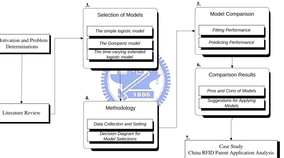
Chapter 1 of this paper provides an introduction and Chapter 2 discusses literatures about technology forecasting methods, the challenges of forecasting short product lifecycles and traditional and newly developed technology forecasting models including the simple logistic model, the Gompertz model, and the time-varying extended logistic model. Chapter 3 presents the methodology and the analytical process of this study. Chapter 4 describes comparison results of the models’ prediction performances and provides the suggestions for using the models. Chapter 5 provides an empirical case of China RFID patent analysis. The last chapter provides a summary and conclusion as well as the limitations of the study. Figure 1 presents the research framework and process of this dissertation.
Motivation and Problem Determinations
Case Study
China RFID Patent Application Analysis Selection of Models
1.
3. 5.
7. 2.
The simple logistic model The Gompertz model The time-varying extended
logistic model Model Comparison Fitting Performance Predicting Performance 6. Comparison Results
Pros and Cons of Models Suggestions for Applying
Models
Literature Review
4.
Methodology
Data Collection and Setting Decision Diagram for
Model Selections
2. Literature Review
The lifecycle concepts have been used in different field. Nieto, Lopez, and Cruz, (1998) proposed that the lifecycles of technologies, industries and products follow similar S-shape curve which is the pattern of biological growth of living beings. Therefore, the authors relate the growth curve models to lifecycle management. However, the product lifecycle analysis focuses on the evolution of sales of products to provide marketing and management strategies for firm and business unit; while technology lifecycle analysis concentrates on the effects of evolution of given technology to generate strategies for production and technology management. This research applied the concepts that the product lifecycle and technology lifecycle can both be forecasted using growth curve models, a kind of technology forecasting methods.
Furthermore, this research studies the lifecycle of technology products, which are different with durable or service products. The lifecycle of technology products become shorter and shorter as technology improves, since the new technology products are easily to be developed and to replace the old ones. The present situation makes the management of short lifecycle products become more important than before. Thus, forecasting technology product lifecycles can be viewed as forecasting short product lifecycles. Kurawarwala & Matsuo (1996) state that the duration of short product lifecycle usually is one to two years. Hasted and Ehlers (1989) define a small dataset as the dataset which covers only short time intervals with fewer than 30 data points. Therefore, I follow these definitions and define the product lifecycle of one or two years with less than thirty data points as short product lifecycle. This chapter begins with the discussion of technology forecasting models, and then the literatures of forecasting short lifecycle products are reviewed. Finally, the three growth curve models used in
this research are presented.
2.1 Technology Forecasting Methods
In general, technology forecasting methods can be classified into quantitative and qualitative methods. Martino (1993) outlines ten forecasting methods, including Delphi, analogy, growth curves, trend extrapolation, correlation methods, causal models, probabilities methods, environmental monitoring, combining forecasts, and normative methods. The following section will separates these methods into quantitative and qualitative categories and discuss their contents and applications. Furthermore, the criteria of selecting forecasting models are also presented.
2.1.1 Qualitative forecasting methods
Qualitative forecasting methods are those forecasting methods do not use mathematical or statistical technologies, therefore, based on this definition, Delphi, analogy, environmental monitoring, and normative methods.
1. Delphi
Delphi is a kind of expert opinion methods and a series of questionnaire are used to collect the panelists’ opinion. Panelists are the experts familiar with the specific industries or problems that the research focuses on. Delphi is usually applied in the three conditions. The first condition is there is no historical data can be used; the second condition is when important external factors happen and the previous data can not be applied, and the third condition is when ethical or moral considerations dominate the development of technology (Martino, 1993). Delphi can gain the extensive opinions and panelists do not need to interact with each other, so they won’t be influenced by others and shift their opinions. Levary & Han (1995) suggest that all participants should be
experts about the given technology.
2. Analogy
The assumption of analogy is if the background or characteristics of two technologies are similar, they may have the same similar development trends; therefore, the forecast can be based on historical analogy. There are nine dimensions need to be taken into consideration when applying analogy, and they are technological dimension, economic dimension, managerial dimension, political dimension, social dimension, cultural dimension, intellectual dimension, religious-ethical dimension, and ecological dimension.
3. Environmental monitoring
A breakthrough of a technology is the end result of a chain and is not easy to predict. Environmental monitoring method then can be applied to detect the breakthrough and is a systematic forecast method that involves evaluating kinds of environmental sectors, including the technological sector, the economic sector, the managerial sector, the political sector, the social sector, the cultural sector, the intellectual sector, the religious-ethical sector, and the ecological sector (Martino, 1993).
4. Normative methods
Normative methods are the goal oriented forecast methods and are different from the exploration forecasts which are used to predict future development using the previous or present data. Setting a goal is the first task of applying the methods, and therefore, when, who, what, why, and the know-how of a technology should be clearly set. The representative models of normative methods are relevance trees, morphological models, and mission flow diagrams.
2.1.2 Quantitative forecasting methods
When a forecasting method uses mathematical or statistical data to forecast, the method is a kind of quantitative forecasting methods, such as growth curve, trend extrapolation, correlation method, causal models, probabilities methods, and combining forecasts. Valid time series datasets are the key to forecasting accuracy of quantitative methods and forecasters believe that the historical data present a logical trend for future and can be used to project the prospect development (Martino, 2003).
1. Growth curve model
Growth curve model, also names as S-curve model, is often applied to forecast the technology or product lifecycles since the growth of technology/product lifecycle is usually follows an S-shape curve. Growth curve model uses the historical date to forecast the future performance of the technology or product. Three assumptions need to be fulfilled before applying the traditional growth curve models. The first assumption is the upper limit to the growth curve is known; the second assumption is the chosen growth curve to be fitted to the historical data is the correct one, and the third assumption is the historical data gives the coefficients of the chosen growth curve formula correctly (Martino, 1993). Since the growth curve model is the main method of this study, the detailed discussion will be presented in the next section.
2. Trend extrapolation
Every technology will reach its maximum performance level, i.e. the upper limit, and new technology will appear to replace the old one. Trend extrapolation is used to forecast the progress beyond the upper limit of the existing technology. Even we do not know what and when the breakthrough technology will be, the previous technology development and historical data can be used to forecast the future technology. However,
if a technology is known that it will not have further development, the trend extrapolation is not suitable to be used. Levary & Han (1995) suggest every trend extrapolation model need to have assumptions and satisfying these assumptions is the determinate of forecast accuracy.
3. Correlation method
Correlation method is similar to analogy method. The predicted technology should have the similar characteristics to the previous technology. However, correlation method uses the quantitative historical data of the similar technology to forecast and analogy method uses qualitative dimension to project the similar technology development. Martino (1993) introduces several correlation methods for forecasting a technology, including a technological precursor, cumulative production, total capacity, and economic factors.
4. Causal models
Causal models are used to realize the reasons that induced the development of the technology. Once the reasons are defined, the future development can be forecasted. Martino (1993) introduces three types of causal models. The first type is technology-only models, such as the growth of scientific knowledge and a universal growth curve, and these models assume that the technological changes can be explained by internal factors of the system of technology. The second type is techno-economic models and the assumption of these models is that the technological development is caused by economic factors. The third type of causal models is economic and social models which assume economic and social factors are the reasons that induce the technological development, and KSIM and differential equations models are the major representative models.
5. Probabilities methods
Probabilistic methods are used to predict the range that a technology can develop and reach to and the probability distribution over the range. Martino (1993) outlines two types of the probabilistic forecasts. The first type of methods relates a range of possible future values and the probability distribution over the range and the second type of probabilistic method is based on a probability distribution of the factors that produce technological changes. Probabilistic forecasts can be operated using simulation techniques.
6. Combining forecasts
Every forecast method has its advantages and disadvantages, and therefore, different methods can be combined to improve the accuracy of prediction. Combining forecasts then are popular in predictors to avoid problems of selecting only one forecast method. Researchers should study the strengths and weakness of individual forecast methods to know how to combine different forecasts to reach better predictions. Usually combining forecasts can be quantitative and/or qualitative methods. Trend and growth curves combination, trend and analogy, components and aggregates, cross-impact models, and scenario analysis are most used combining methods. Levary & Han (1995) suggest the cross-impact analysis should be applied when the factors that affect the future technology are known, and the scenario developers should expert all aspect of the technology.
2.1.3 The selection of technological forecasting models
Levary and Han (1995) outline six factors that influence the selection of forecasting methods. First, money available for development, the more money invest in the given technology, the more opportunity the technology can be realized and the
shorter the development time. Second, data availability, what data researchers can retrieve affect the methods selection. Third, data validity also affects the choice. Fourth, uncertainty surrounding the success of technological development, some technology forecasting methods are suitable to high uncertainty situation while other are not. Fifth, if similarity of proposed and existing technologies is high, analogy or correlation methods can be applied. Finally, number of variables affecting the development of technology, the more influence factors, the more complex models should be applied, and therefore, combining forecast methods may be needed.
Young (1993) applies nine growth models to determine the procedure of selecting an appropriate growth models. The author concludes that the most important procedure is to identify the characteristics of datasets before fitting the data into the growth curve models. Predictors intend to apply growth curve model need to know the knowledge of upper limit, to observe whether the fifty percent takeover point has been achieved in the dataset, and to study the length of datasets.
2.2 Forecasting Short Product Lifecycles
Short product lifecycles of one or two years have become more common in high technology and fashion-based industries which need to continuously introduce new consumer products to remain competitive (Kurawarwala & Matsuo, 1996; Zhu & Thonemann, 2004). New electronic products with more functions, faster speed, and finer quality are continuously being introduced and quickly replace models which may only be one year old. Quell, Olshavsky, and Michaels (1981) analyzed 37 types of home appliance from 1922 to 1979 and demonstrated that the shortening of product life cycles is an important issue for product designers and planners. Given the reality of this market condition, the development of new forecasting techniques will improve the competitive
response and manufacturing strategy of companies.
In 1969, Bass (1969) proposed a diffusion model to forecast the sales volume of new products that used the adoption rates of innovators and imitators. Innovators are buyers that are not influenced by the previous buyers when making purchase decisions while imitators are those who are influenced by earlier buyers. The Bass model has been widely applied by practitioners and modified by researchers to forecast short product lifecycles. Kurawarwala and Matsuo (1996) proposed a growth model that forecasts the seasonal sales volume demand of short product lifecycles based on the Bass diffusion model. Thirty-eight monthly data points for five different personal computer products were used to estimate seasonal demand and to compare the fit and forecast performance for three models. The measures used for model comparison were the sum of squared error (SSE), the root mean squared error (RMSE), and the mean absolute deviation (MAD). Zhu and Thonemann (2004) used the discrete version of the Bass diffusion model and improved on Kurawarwala and Matsuo (1998) model to develop an adaptive forecasting algorithm. The demand data for a PC manufacturer was used to test the forecasting performance of the algorithm. Chen (2005) proposed an extended logistic model, which is called the time-varying extended logistic model. The researcher use seven durable home appliance datasets to compare the fit and prediction accuracy of the Fisher-Pry model, the Gompertz model, and the time-varying extended logistic model. Chen concluded that the proposed extended logistic model had better fit and forecast performances while the Fisher-Pry can have fine fit performance when the product has reached 100% penetration rate. Chen also suggested that the Gompertz model should be used only when the right capacity can be correctly set. This research uses the model from Chen’s study to demonstrate that the extended logistic model improved the forecast of both long and short lifecycle datasets.
Lackman (1993) reported that the simple logistic and the Gompertz models are suitable for forecasting high technology products. Morrison (1996) also showed that the simple logistic and the Gompertz models can be used to forecast the growth of new products. However, when the author applied the models, the upper limit was set subjectively. Bengisu and Nekhili (2006) used the simple logistic and the Gompertz models to predict emerging technologies using publications and patents from science and technology databases and Boretos (2007) used the simple logistic model to show that the diffusion of mobile phone technology follows an S-curve.
Meade and Islam (1995) compared seventeen growth models based on 25 time series datasets describing the telecommunications market. Their literature review shows that the simple logistic model is the most widely used. The authors conclude that basic forecasting models using two or three parameters, such as the simple logistic and Gompertz model, offer the best forecasting performance. Their research used datasets for traditional land-line telephones to compare forecasting models. However, the classic telephone introduced in the 1960s and which remained in use through the 1980s has a long product lifecycle that lasted over 30 years. When there are sufficient data points, the trajectory of the product growth curve is clear and the point of inflection can be calculated. If the point of inflection can be estimated, then the upper limit of the simple logistic and the Gompertz models can also be estimated. The simple logistic model is symmetric about the point of inflection. So if the inflection point is defined, the upper limit is twice the market share that occurs at the inflection point. For the Gompertz model, the point of inflection occurs at 37.79% of the upper limit and the upper limit can also be calculated when the inflection point is found. Bengisu and Nekhili (2006) showed that the simple logistic and the Gompertz models are quite valid if the upper limit is correctly identified. However, the data points may not be sufficient (too few) to
see the point of inflection and to set the correct upper limit when forecasting short lifecycle products. Therefore, a model with more parameters, for example, the time-varying extended logistic model, is needed to project the trajectory of the growth curve. The time-varying extended logistic model uses a dynamic upper limit that can be estimated from the data.
2.3 Growth Curve Models
Most biological growth follows an S-shape curve or logistic curve which best models growth and decline over time (Meyer & Ausubel, 1999). Since the lifecycle of technology and technology based products is similar to biological growth, the growth curve models are used to capture the future development of the technology or products. There are many growth curve models, and Meade & Islam (1998) classify twenty-nine growth curve models into four categories: trend curve models, linearised trend models, nonlinear auto-regressive models, and hybrid models. However, the simple logistic and the Gompertz models are the two most applied models when forecasting the lifecycle of technology products. Nevertheless, the limitation of setting the correct upper limit for these two traditional models increases the difficulties of applying the models. Therefore, the extended logistic model with dynamic upper limit is introduced to see if this model can reach better performances in forecasting short lifecycle products than the two traditional models.
2.3.1 Simple logistic curve model
The simple logistic model is widely used for technology forecasting. Many new forecasting models were proposed based on the simple logistic model and include innovations such as the Bass diffusion model and extended logistic model (Meade & Islam, 1995). The most important characteristic of simple logistic model is that it is
symmetric about the point of inflection. This feature indicates that the process which will happen after the point of inflection is the mirror image of the process that happened before the point.
The model for the simple logistic curve is controlled by three coefficients, a, b, and L is expressed as: bt t ae L y − + = 1 (1)
where is the value of interest, is the maximum value of , a describes the location of the curve, and b controls the shape of the curve. To estimate the parameters for a and b, the equation of the simple logistic model is transformed into a linear function using natural logarithms. The linear model is expressed as:
t
y L yt
(
y L y)
( )
a btYt =ln t − t =−ln + (2)
where the parameter a and b are then estimated using a simple linear regression. The simple logistic model (equation 1) and the linear model (equation 2) are quoted from Martino’s book (Martino, 1993) and the derivations are shown in Appendix 1.
2.3.2 Gompertz model
The Gompertz model was first used to calculate mortality rates in 1825 and has been widely applied to technology forecasting (Martino, 1993). Although the Gompertz curve is similar to the simple logistic curve, it is not symmetric about the inflection point which occurs at t=
(
ln( )
b k)
. The Gompertz model reaches the point of inflection early in the growth trend and is expressed as:bt
ae t Le
y = − − (3)
b. Similar to the methodology of estimating the parameters of the simple logistic model, natural logarithms are used to transform the original Gompertz model to linear equation:
(
)
(
L y)
( )
a btYt =ln ln t =ln − (4)
and then the parameters are estimated (Martino, 1993). Equation (3) and equation (4) quoted from Martino’s book and the derivations are shown in Appendix 2.
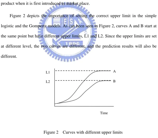
Although the predictive performance of the simple logistic model and the Gompertz model has been validated by many researchers (Meade & Islam, 1998), the models have definite limitations when used to forecast short product lifecycles. The reason is that it is almost impossible to estimate the correct upper limit for a new product when it is first introduced to market place.
Figure 2 depicts the importance of setting the correct upper limit in the simple logistic and the Gompertz models. As can been seen in Figure 2, curves A and B start at the same point but have different upper limits, L1 and L2. Since the upper limits are set at different level, the two curves are different, and the prediction results will also be different. L1 Time L2 A B
2.3.3 Time-varying extended logistic model
The simple logistic model and the Gompertz model assume that the capacity of technology adoption is fixed and there is an upper bound to growth for these models. However, the adoption of new technology is seldom constant and changes over time. Therefore, researchers have proposed a dynamic carrying capacity and the carrying capacity can be any function (Meyer & Ausubel, 1999; Cohen, 1995). As shown by Meyer & Ausubel (1999), the original form of simple logistic model is written as:
⎟ ⎠ ⎞ ⎜ ⎝ ⎛ − × × = L y y L b dt dy t t t 1 (5)
Let α =b×L and replace the constant L in equation (5) with a function , and then the equation (5) is extended to:
( )
t k( )
⎟ ⎠ ⎞ ⎜ ⎝ ⎛ − × = t k y y dt dy t t t 1 α (6)where L is the upper limit of the logistic curve and k
( )
t is the time-varying capacity function similar to the logistic curve.In Meyer and Ausubel’s study, a special k
( )
t was set to represent a technology which has a bio-logistic growth rate. Chen (2005) follows the concept of Meyer and Ausubel and proposes a time-varying extended logistic model with dynamiccapacityk
( )
t . This thesis applies Chen’s setting of k( )
t and uses the extended logistic model to forecast the future trend of technology product. The setting of in Chen’s is expressed as( )
t k( )
ct e d t k = 1− × − (7)and c and d are parameters that are estimated. Chen defines the value of d can be any number and the value of c is larger than zero. The research also assumes that the
penetration rate capacity will fluctuate with time and may reach 100% but may also be as low as 30% or 50%. The reason for this assumption is that some new products may be introduced to the market and substitute older products. Thus, a product may not always achieve 100% market penetration and may be replaced earlier than expected.
Finally, the time-varying extended logistic model is expressed as:
( )
bt ct bt t e a e d e a t k y − − − + × × − = × + = 1 1 1 (8)where is the capacity that fluctuates with time, and a, b, c, and d are the parameters computed using a nonlinear least squared estimation method provided by a statistic software package like SYSTAT. When this model is tested using sales volume data, the equation is changed to:
( )
t k bt ct t t e a e d m y m N − − × + × − = = 1 1 * * (9)where Nt is cumulative volume by time t, and the coefficient m represents the total market sales which is estimated using nonlinear least squares method.
The time-varying extended logistic model is similar to the Bass diffusion model which can be viewed as a special case of this model. The Bass model was developed for predicting sales volume, whereas the time-varying extended logistic model can be modified to predict sales volume as well as other proxies including market penetration rates. Therefore, the time-varying extended logistic model was selected for evaluation over the Bass model.
There is little published research which compares the performance of forecasting models used on both long and short product lifecycle datasets. Thus, to see if the time-varying extended logistic model with dynamic upper limit has better fit and prediction results over the simple logistic and the Gompertz models, this study applies
Chen’s time-varying extended logistic model and compares the performance of the three models. Moreover, based on the comparison results, this research outlines the pros and cons of the three models and proposed a models selection chart to provide a suggestion of applying the three forecasting models.
3. Methodology
This chapter presents the methodology used in this study, including the data collection and setting, the analytical process for comparing the fitting and predicting performances of forecasting models, and the proposed model selection procedure.
3.1 Data Collection
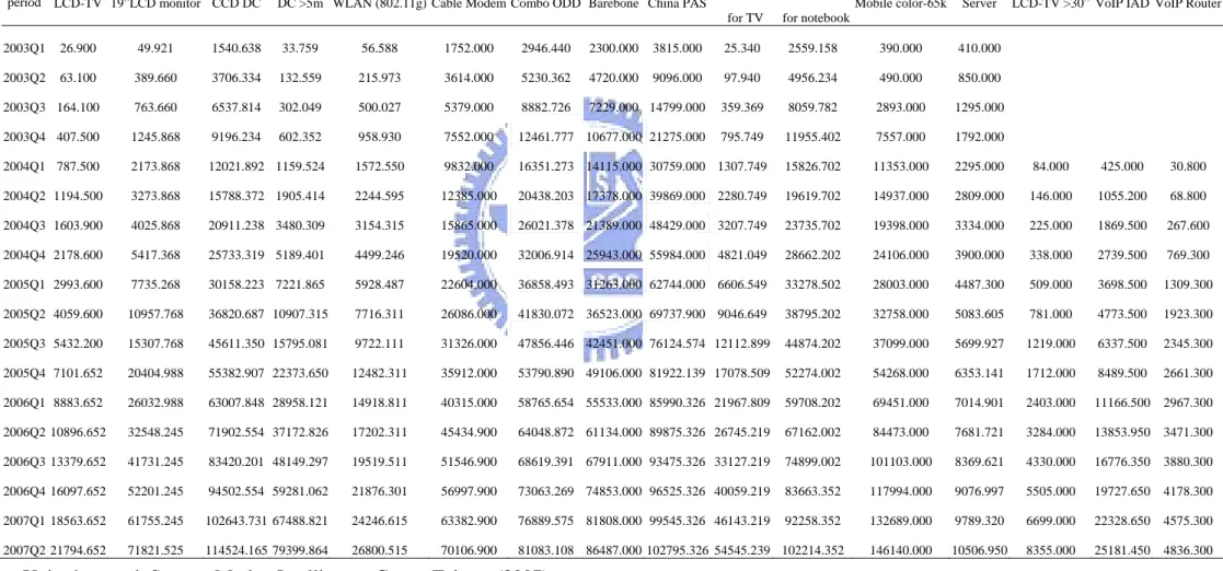
Twenty-two time-series datasets describing Taiwan penetration rate and cumulative sales volume of electronic products were collected to test the forecast accuracy of the simple logistic model, the Gompertz model and the time-varying extended logistic model. In order to see what kinds of products can be fitted and forecasted by the three models, the datasets are not pre-selected. The datasets for market penetration rates were providing by the Directorate General of Telecommunications and Chunghwa Telecom Co. (2007) and the Directorate General of Budget (2007). The market penetration rate datasets cover six products including color TVs, telephones, washing machines, Asymmetric Digital Subscriber Lines (ADSL), mobile Internet subscribers, and broadband networks. The cumulative sales volume datasets were provided by the Taiwan Market Intelligence Center (2007). These datasets cover sixteen products including LCD-TV, 19 inch LCD monitors, digital cameras with Charge Coupled Device image sensors (CCD DC), digital cameras with more than 5 million pixels (DC >5m), 802.11g wireless local area networks devices (WLAN 802.11g), cable modems, combo optical disk drives (combo ODD), Barebone computers (Barebone), China personal wireless access systems (China PAS), LCD panels for TV, LCD panels for notebooks, color mobile phones with 65K pixels (color-65k mobile phone), servers, over 30 inch wide LCD-TVs (LCD-TV >30”), Voice over Internet Protocol Integrated Access Devices (VoIP IAD), and Voice over Internet protocol (VoIP) routers.
3.2 Data Settings
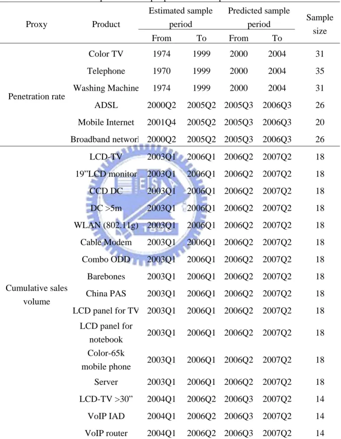
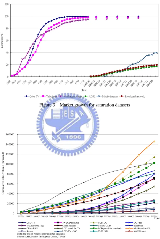
As shown in Table 1, the estimated sample period, predicted sample period, and sample sizes are presented. The data for color TVs, telephones and washing machines are yearly data points. Since the sample period for these data is greater than 30 years, these products depict a complete product life cycle (Figure 3). This research classifies the data for color TVs, telephones and washing machines as long product lifecycles with large datasets for forecasting. The other datasets (ADSL, mobile Internet subscribers, etc.) represent products rapidly brought to market and are categorized as short lifecycle products with limited or small (less than 30 data points) datasets for forecasting. Table 2 lists the detail data of cumulative sales volume dataset.
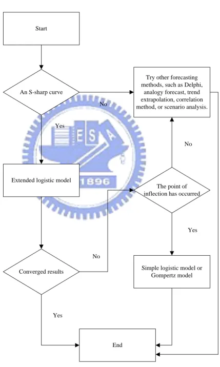
Figure 3 shows the penetration rate for the six products and Figure 4 shows the cumulative sales volume for the sixteen short lifecycle products. Figure 3 shows that color TVs, telephones, and washing machines have entered the mature stage of the product life cycle. Therefore, a clear upper limit for these products can be set. On the other hand, the curves for ADSL, mobile Internet subscribers, and other short lifecycle products are still evolving, making it difficult to define the stage of product life cycle or to predict when these products will stop growing.
For the long product lifecycle datasets, the upper limit is set at 100%. For the short product lifecycle datasets, different upper limits are set to achieve the best estimates. The possible upper limit for the short lifecycle is set at 3 different levels to include optimistic, a conservative, and a pessimistic settings. An optimistic upper limit means that the product is new to the market and has potential to grow. A pessimistic setting means that the product almost reached the upper limit to market growth. Between the optimistic and pessimistic limits is the conservative setting. The conservative setting
models a product that has been in the market for a while and has reached about one-third or one-half of the upper limits to growth.
Table 1 Estimated and predicted sample period and sample size Estimated sample period Predicted sample period Proxy Product From To From To Sample size Color TV 1974 1999 2000 2004 31 Telephone 1970 1999 2000 2004 35 Washing Machine 1974 1999 2000 2004 31 ADSL 2000Q2 2005Q2 2005Q3 2006Q3 26 Mobile Internet 2001Q4 2005Q2 2005Q3 2006Q3 20 Penetration rate Broadband network 2000Q2 2005Q2 2005Q3 2006Q3 26 LCD-TV 2003Q1 2006Q1 2006Q2 2007Q2 18 19”LCD monitor 2003Q1 2006Q1 2006Q2 2007Q2 18 CCD DC 2003Q1 2006Q1 2006Q2 2007Q2 18 DC >5m 2003Q1 2006Q1 2006Q2 2007Q2 18 WLAN (802.11g) 2003Q1 2006Q1 2006Q2 2007Q2 18 Cable Modem 2003Q1 2006Q1 2006Q2 2007Q2 18 Combo ODD 2003Q1 2006Q1 2006Q2 2007Q2 18 Barebones 2003Q1 2006Q1 2006Q2 2007Q2 18 China PAS 2003Q1 2006Q1 2006Q2 2007Q2 18 LCD panel for TV 2003Q1 2006Q1 2006Q2 2007Q2 18 LCD panel for notebook 2003Q1 2006Q1 2006Q2 2007Q2 18 Color-65k mobile phone 2003Q1 2006Q1 2006Q2 2007Q2 18 Server 2003Q1 2006Q1 2006Q2 2007Q2 18 LCD-TV >30” 2004Q1 2006Q2 2006Q3 2007Q2 14 VoIP IAD 2004Q1 2006Q2 2006Q3 2007Q2 14 Cumulative sales volume VoIP router 2004Q1 2006Q2 2006Q3 2007Q2 14 Source: Directorate General of Budget, Directorate General of Telecommunications and Chunghwa Telecom Co. (2007), and Market Intelligence Center Taiwan (2007).
Table 2 Cumulative sales volume dataset
Products Sample
period LCD-TV 19”LCD monitor CCD DC DC >5m WLAN (802.11g) Cable Modem Combo ODD Barebone China PAS
LCD panel for TV
LCD panel for notebook
Mobile color-65k Server LCD-TV >30” VoIP IAD VoIP Router
2003Q1 26.900 49.921 1540.638 33.759 56.588 1752.000 2946.440 2300.000 3815.000 25.340 2559.158 390.000 410.000 2003Q2 63.100 389.660 3706.334 132.559 215.973 3614.000 5230.362 4720.000 9096.000 97.940 4956.234 490.000 850.000 2003Q3 164.100 763.660 6537.814 302.049 500.027 5379.000 8882.726 7229.000 14799.000 359.369 8059.782 2893.000 1295.000 2003Q4 407.500 1245.868 9196.234 602.352 958.930 7552.000 12461.777 10677.000 21275.000 795.749 11955.402 7557.000 1792.000 2004Q1 787.500 2173.868 12021.892 1159.524 1572.550 9832.000 16351.273 14115.000 30759.000 1307.749 15826.702 11353.000 2295.000 84.000 425.000 30.800 2004Q2 1194.500 3273.868 15788.372 1905.414 2244.595 12385.000 20438.203 17378.000 39869.000 2280.749 19619.702 14937.000 2809.000 146.000 1055.200 68.800 2004Q3 1603.900 4025.868 20911.238 3480.309 3154.315 15865.000 26021.378 21389.000 48429.000 3207.749 23735.702 19398.000 3334.000 225.000 1869.500 267.600 2004Q4 2178.600 5417.368 25733.319 5189.401 4499.246 19520.000 32006.914 25943.000 55984.000 4821.049 28662.202 24106.000 3900.000 338.000 2739.500 769.300 2005Q1 2993.600 7735.268 30158.223 7221.865 5928.487 22604.000 36858.493 31263.000 62744.000 6606.549 33278.502 28003.000 4487.300 509.000 3698.500 1309.300 2005Q2 4059.600 10957.768 36820.687 10907.315 7716.311 26086.000 41830.072 36523.000 69737.900 9046.649 38795.202 32758.000 5083.605 781.000 4773.500 1923.300 2005Q3 5432.200 15307.768 45611.350 15795.081 9722.111 31326.000 47856.446 42451.000 76124.574 12112.899 44874.202 37099.000 5699.927 1219.000 6337.500 2345.300 2005Q4 7101.652 20404.988 55382.907 22373.650 12482.311 35912.000 53790.890 49106.000 81922.139 17078.509 52274.002 54268.000 6353.141 1712.000 8489.500 2661.300 2006Q1 8883.652 26032.988 63007.848 28958.121 14918.811 40315.000 58765.654 55533.000 85990.326 21967.809 59708.202 69451.000 7014.901 2403.000 11166.500 2967.300 2006Q2 10896.652 32548.245 71902.554 37172.826 17202.311 45434.900 64048.872 61134.000 89875.326 26745.219 67162.002 84473.000 7681.721 3284.000 13853.950 3471.300 2006Q3 13379.652 41731.245 83420.201 48149.297 19519.511 51546.900 68619.391 67911.000 93475.326 33127.219 74899.002 101103.000 8369.621 4330.000 16776.350 3880.300 2006Q4 16097.652 52201.245 94502.554 59281.062 21876.301 56997.900 73063.269 74853.000 96525.326 40059.219 83663.352 117994.000 9076.997 5505.000 19727.650 4178.300 2007Q1 18563.652 61755.245 102643.731 67488.821 24246.615 63382.900 76889.575 81808.000 99545.326 46143.219 92258.352 132689.000 9789.320 6699.000 22328.650 4575.300 2007Q2 21794.652 71821.525 114524.165 79399.864 26800.515 70106.900 81083.108 86487.000 102795.326 54545.239 102214.352 146140.000 10506.950 8355.000 25181.450 4836.300
0 20 40 60 80 100 120 1964 1970 1974 1976 197 8 1980 1982 198 4 1986 1988 1990 1992 1994 1996 1998 2000 .06 2000 .12 2001 .06 2001 .12 2002 .06 2002.1 2 2003 .06 2003 .12 2004.0 6 2004.1 2 2005 .06 2005 .12 2006.0 6 Time Satu ra ti on ( % )
Color TV Telephone Washing machine ADSL Mobile internet Broadband network Figure 3 Market growth for saturation datasets
0 20000 40000 60000 80000 100000 120000 140000 160000 2003Q1 2003Q2 2003Q3 2003Q4 2004Q1 2004Q2 2004Q3 2004Q4 2005Q1 2005Q2 2005Q3 2005Q4 2006Q1 2006Q2 2006Q3 2006Q4 2007Q1 2007Q2 Time C u m u la ti v e sal es vo lu m e ( th o u sa nd ) LCD-TV 19”LCD monitor CCD DC DC >5m
WLAN (802.11g) Cable Modem Combo ODD Barebone
China PAS LCD panel for TV LCD panel for notebook Mobile color-65k
Server LCD-TV >30” VoIP IAD VoIP Router
Note: the unit of wireless internet is ten thousand. Source: ASIP, Market Intelligence Center, Taiwan
The penetration rate datasets use upper limits of 100%, 50%, and 30%. However, since the current penetration rate of the mobile Internet is 40%, the pessimistic setting is change to 50% and conservative upper limit is changed to 60%. For the cumulative sales volume datasets, the upper limit is set based on the multiple of the most recent observation as recommended by Meade and Islam (1998). The optimistic, conservative, and pessimistic upper limits are 5 times, 3 times, and 1.5 times the most recent observation which is based on the cumulative sales volume of the second quarter in 2007. In fact, 5 times the most recent observation means that the proportion of the current cumulative sales volume to maximum sales volume (upper limit) is 20%. Thus, the current cumulative sales volume only reaches 20% of the upper limit and there is still 80% of the maximum sales volume remaining to sell. So the setting of 5 times the most recent observation is an optimistic setting. A pessimistic setting of the cumulative sales volume dataset is set at 1.5 times the most recent observation. Using the cable modem dataset as an example, the most recent cumulative sales volume is 70,106,900 units and the pessimistic upper limit is 105,160,350 units. This means that the current cumulative sales volume has already reached two-third of the upper limit and has entered the mature stage of the product lifecycle.
3.3 Model Comparison Analytical Process
In order to test the forecast accuracy of the simple logistic, Gompertz, and the time-varying extended logistic models, the analytical process is divided into two steps.
Step 1: Model estimation
The first step is used to estimate the models. After reserving the last five data points to test forecast accuracy of the simple logistic, Gompertz, and the time-varying extended logistic models, the remaining data points were used to fit the three models. For the simple logistic and the Gompertz model, equation (2) and (4) are used to estimate coefficients using a simple linear regression. For the time-varying extended logistic model, the coefficients of the models are estimated using nonlinear least squares with SYSTAT statistical software (Chen, 2003). After the coefficients were computed and the models fitted, the estimated values were calculated.
Step 2: Fit and forecast performance
After the models are constructed, the fit and forecast performance between the three models is conducted. The test consists of checking residuals between actual values and estimated values to measure model performance (Kurawarwala & Matsuo, 1996; Meyer & Ausubel, 1998). Two measurements, mean absolute deviation (MAD) and root mean square error (RMSE) are used to calculate residuals.
For the simple logistic and the Gompertz models, the upper limit must be set to obtain accurate results. Setting different upper limit levels of these two models will achieve different prediction results and the fit and predict performance will also be influenced. Thus, several upper limits of the simple and the Gompertz models were set to determine which upper limit would yield the best fit performance.
For forecast performance, the derived models are used to forecast the last five data points of the datasets. In this study, the Mean Absolute Deviation (MAD) and Root Mean Square Error (RMSE) are used to measure performance as recommended in the literature (Kurawarwala & Matsuo, 1996; Meyer & Ausubel, 1998; Islam & Meade, 1996). The mathematical representations are shown below:
n y y MAD T t t t
∑
= − = 1 ˆ (10)(
)
n y y RMSE T t t t∑
= − = 1 2 ˆ (11)where is the actual value at time t, is the estimate at time t, and n is the number of observations. These measurements are based on the residuals, which represent the distance between real data and predictive data. Consequently, if the values of these measures are small, then the fit and prediction performance is acceptable.
t
y yˆt
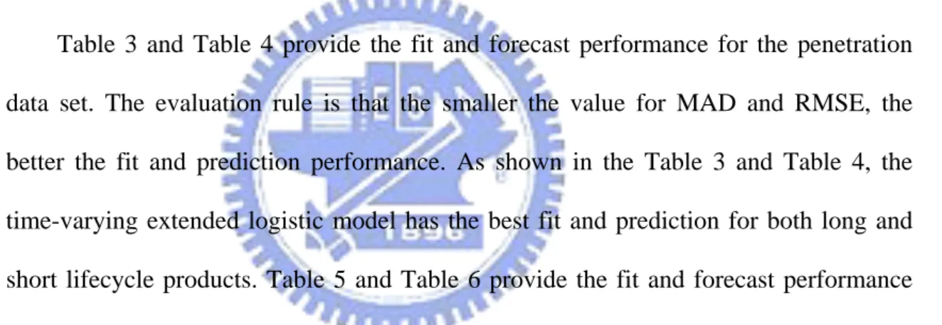
3.4 The Proposed Model Selection Procedure
According to previous literatures, this research proposed a decision chart for how to select a forecasting model among the simple logistic model, the Gompertz model and the time-varying extended logistic model. Figure 5 presents the decision flow for selecting the forecasting models. This study assume that the time-varying extended logistic model will have the best forecasting result, so it is firstly recommended for predicting the technology product life cycle. Extended logistic model can be used to forecast the future trend at the early lifecycle stage even when the point of inflection of the growth curve has not occurred. Young (1993) suggests that the predictors need to study the characteristics of datasets. Therefore, in Figure 5, the first step is to see if the
S curve is identified, then the time-varying extended logistic model can be applied, and if a convergent result can be reached with the extended logistic model, then the prediction process ends. However, since there are more parameters needed to be estimated in the time-varying extended logistic model, it may sometimes produce a non-convergent result. Thus, due to the characteristics and limitations of the extended logistic model, the data which can be plotted as an S-curve with more than fifteen data points is strongly recommended when using the extended logistic model. Besides, because the time-varying extended logistic model is developed based on S-curve, flat curves or curves with obvious jump are not suitable to be forecasted using extended logistic model.
Under the non-convergent condition, predictors can check whether the point of inflection of the S-curve has occurred or not. If an inflection point occurred, the capacity of the simple logistic and Gompertz models can be estimated, and then these two models can be applied. Therefore, researchers can select the simple logistic or the Gompertz models based on their understandings of the product and the market. My suggestion is that if the researchers think the market has more potential to develop in the future, then the Gompertz model is more suitable for that kind of products than the simple logistic model since the inflection point of the Gompertz model occurs at 37.79% of the upper limit, and there will be another 62.21% to grow. For the simple logistic model, it is a symmetric model and its point of inflection happens at the half of the curve, there will be only 50% potential to grow after the inflection point. Besides, when the analytical data is patent document data, the simple logistic model is suggested to use since it is the most applied model in the previous patent analysis literatures. However, if an inflection point has not occurred, the growth curve methods are not suitable for technology forecasting, and other technology forecasting methods, such as
Delphi, analogy forecast, trend extrapolation, correlation method, or scenario can be tried to use (Martino, 1993). This decision process will be demonstrated with a RFID case study presented in next chapter and the forecasting results will be verified with industrial experts to see if the proposed procedure has the validity.
Start
An S-sharp curve
Extended logistic model
Try other forecasting methods, such as Delphi,
analogy forecast, trend extrapolation, correlation method, or scenario analysis.
The point of inflection has occurred
Simple logistic model or Gompertz model End Yes Yes Yes No No No Converged results
4. Comparison Results
This chapter discusses the comparison results for evaluating the simple logistic, the Gompertz, and the time-varying extended logistic models. The fit and forecast performances are evaluated by using Mean Absolute Deviation (MAD) and Root Mean Square Error (RMSE). A sign test is also performed to show that there are statistically significant differences for the comparison results to reach more precise conclusions. Finally, suggestions for applying the three models and a decision diagram for model selection are presented for future researchers.
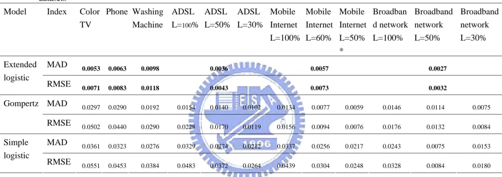
4.1 Comparison of Performances
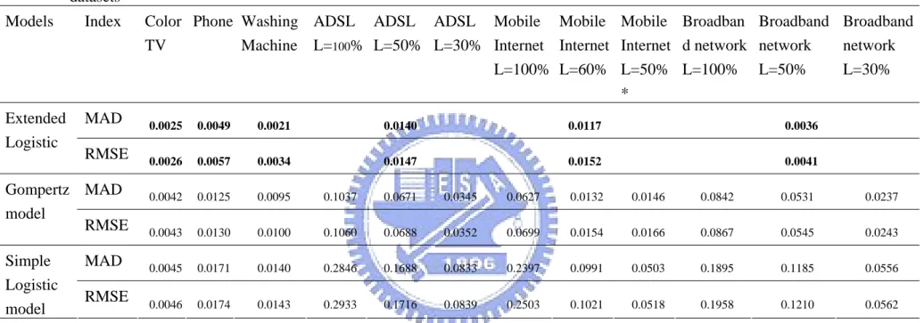
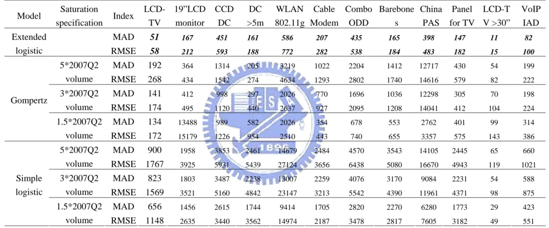
Table 3 and Table 4 provide the fit and forecast performance for the penetration data set. The evaluation rule is that the smaller the value for MAD and RMSE, the better the fit and prediction performance. As shown in the Table 3 and Table 4, the time-varying extended logistic model has the best fit and prediction for both long and short lifecycle products. Table 5 and Table 6 provide the fit and forecast performance for the cumulative sales volume data set. Table 5 shows that time-varying extended logistic model has the best fit performance for all products. Table 6 shows that the time-varying extended logistic model has the best forecast performance for the majority of the products.
Table 7 summarizes the comparative results of the time-varying extended logistic model, the simple logistic and the Gompertz models. The fit and forecast performance are compared and ranked using the root mean square error (RMSE) which is widely used for measuring the performance (Kurawarwala & Matsuo, 1996; Meyer & Ausubel, 1998; Cohen, 1995). As can be seen in Table 7 the time-varying extended logistic model has the best predictive performance for 13 products among the 18 products for
which the model converged. The model has the second best predictive performance for 4 products, and the worst predictive performance for LCD-TV >30” data. The Gompertz model predicts best for 4 product datasets and has the second best forecast performance for three models. The simple logistic model only predicts well for the LCD-TV >30” data. In summary, the time-varying extended logistic model is 70% better in prediction than the other models.
Table 3 Fitting performance measures for the time-varying extended logistic, Gompertz, and the simple logistic models: penetration rate datasets
Model Index Color
TV Phone Washing Machine ADSL L=100% ADSL L=50% ADSL L=30% Mobile Internet L=100% Mobile Internet L=60% Mobile Internet L=50% * Broadban d network L=100% Broadband network L=50% Broadband network L=30% MAD 0.0053 0.0063 0.0098 0.0036 0.0057 0.0027 Extended logistic RMSE 0.0071 0.0083 0.0118 0.0043 0.0073 0.0032 MAD 0.0297 0.0290 0.0192 0.0154 0.0140 0.0102 0.0134 0.0077 0.0059 0.0146 0.0114 0.0075 Gompertz RMSE 0.0502 0.0440 0.0290 0.0228 0.0170 0.0119 0.0156 0.0094 0.0076 0.0176 0.0132 0.0084 MAD 0.0361 0.0323 0.0276 0.0329 0.0274 0.0212 0.0337 0.0256 0.0217 0.0243 0.0075 0.0153 Simple logistic RMSE 0.0551 0.0453 0.0384 0.0483 0.0372 0.0264 0.0439 0.0304 0.0248 0.0328 0.0084 0.0180
Note: L: upper limit
*The current saturation rate of mobile Internet is over 30% Boldface number means the best performance among three models.
Table 4 Forecasting performance measures for the time-varying extended logistic, Gompertz, and the simple logistic models: penetration rate datasets
Models Index Color TV Phone Washing Machine ADSL L=100% ADSL L=50% ADSL L=30% Mobile Internet L=100% Mobile Internet L=60% Mobile Internet L=50% * Broadban d network L=100% Broadband network L=50% Broadband network L=30% MAD 0.0025 0.0049 0.0021 0.0140 0.0117 0.0036 Extended Logistic RMSE 0.0026 0.0057 0.0034 0.0147 0.0152 0.0041 MAD 0.0042 0.0125 0.0095 0.1037 0.0671 0.0345 0.0627 0.0132 0.0146 0.0842 0.0531 0.0237 Gompertz model RMSE 0.0043 0.0130 0.0100 0.1060 0.0688 0.0352 0.0699 0.0154 0.0166 0.0867 0.0545 0.0243 MAD 0.0045 0.0171 0.0140 0.2846 0.1688 0.0833 0.2397 0.0991 0.0503 0.1895 0.1185 0.0556 Simple Logistic model RMSE 0.0046 0.0174 0.0143 0.2933 0.1716 0.0839 0.2503 0.1021 0.0518 0.1958 0.1210 0.0562
Note: L: upper limit
*The current saturation rate of mobile Internet is over 30% Boldface number means the best performance among three models.
Table 5 Fitting performance measures for the time-varying extended logistic, Gompertz, and the simple logistic models: cumulative shipment volume data Model Saturation specification Index LCD-TV 19”LCD monitor CCD DC DC >5m WLAN 802.11g Cable Modem Combo ODD Barebone s China PAS Panel for TV LCD-T V >30” VoIP IAD MAD 51 167 451 161 586 207 435 165 398 147 11 82 Extended logistic RMSE 58 212 593 188 772 282 538 184 483 182 15 100 MAD 192 364 1314 205 3219 1022 2204 1412 12717 430 54 199 5*2007Q2 volume RMSE 268 434 1542 274 4634 1293 2802 1740 14616 579 82 222 MAD 141 412 998 297 2026 770 1696 1036 12298 305 70 198 3*2007Q2 volume RMSE 174 495 1120 440 2637 927 2095 1208 14041 412 104 224 MAD 134 13488 989 582 2026 354 678 553 2762 401 99 314 Gompertz 1.5*2007Q2 volume RMSE 172 15179 1226 954 2510 443 740 655 3357 575 143 386 MAD 900 1958 3853 2461 14679 2484 4570 3543 14105 2445 65 660 5*2007Q2 volume RMSE 1767 3925 5931 5439 27124 3656 6438 5080 16670 4943 119 1021 MAD 823 1803 3487 2238 13007 2259 4076 3170 9084 2231 54 588 3*2007Q2 volume RMSE 1569 3521 5160 4842 23147 3213 5542 4390 11961 4371 98 875 MAD 656 1456 2615 1744 9414 1705 2820 2270 6280 1773 29 423 Simple logistic 1.5*2007Q2 volume RMSE 1148 2635 3440 3562 14974 2187 3478 2817 7605 3182 49 551
Table 6 Forecasting performance measures for the time-varying extended logistic, Gompertz, and the simple logistic models: cumulative shipment volume data
Model Saturation specification Index LCD-TV 19”LCD monitor CCD DC DC >5m WLAN 802.11g Cable Modem Combo ODD Barebone s China PAS Panel for TV LCD-T V >30” VoIP IAD MAD 265 6072 923 10068 12030 2253 1878 2040 3115 5217 497 1342 Extended logistic RMSE 301 7758 1157 12434 12505 2911 2029 2153 3305 5846 734 1740 MAD 1820 2372 11176 1813 63530 7910 23077 14504 16194 5076 583 1548 5*2007Q2 volume RMSE 1913 2706 12062 2303 69259 8238 24689 15519 20024 5433 697 2034 MAD 280 6805 3223 5194 32902 3396 15549 7971 11017 604 887 302 3*2007Q2 volume RMSE 360 7814 3452 5582 35553 3419 16541 8421 13492 703 1077 403 MAD 2707 13488 9608 14066 11484 4205 2651 3031 14329 6885 1364 2069 Gompertz 1.5*2007Q2 volume RMSE 3116 15179 10662 15342 12692 5052 2764 3530 14703 7865 1668 2426 MAD 26450 64846 70320 104201 365213 36609 61892 53560 43670 78644 2433 11727 5*2007Q2 volume RMSE 29106 72596 76969 116523 396302 39564 66579 58014 51122 86272 3142 14568 MAD 17740 44268 50134 68273 241342 26680 44945 38728 78007 51581 1643 8250 3*2007Q2 volume RMSE 18836 47682 53567 73370 254235 28212 47516 41109 81173 54536 2060 10020 MAD 6734 16090 16953 25192 86925 9222 16668 13437 29775 19611 295 2516 Simple logistic 1.5*2007Q2 volume RMSE 6786 16182 17113 25473 87717 9271 17002 13582 30183 19761 356 2881