基於龍圖兒之快速大型原型生成

(1)

國立臺灣大學電機資訊學院資訊工程研究所碩士論文

Department of Computer Science and Information Engineering College of Electrical Engineering and Computer Science

National Taiwan University Master Thesis

基於龍圖兒 (Zometool) 之快速大型原型生成 Large-Scale Rapid-Prototyping with Zometool

吳宗鴻 Tsung-Hung Wu

指導教授：陳炳宇博士 Advisor: Bing-Yu Chen, Ph.D.

中華民國 104 年 8 月

August, 2015

(2)

(3)

謝

隨著這篇論文的完成，我的碩士生活也逐漸走到終點，在我的碩士生活中，受到了許多人的幫助，若沒有大家的協助，這份研究肯定無法順利完成，僅以此文向所有人獻上感謝。

首先我要感謝我的指導老師，陳炳宇教授，當年在我進入研究所時，是老師輕鬆詼諧的語氣引導我進入 CMLab 這個大團體，

也總是能在我的研究過程中給予適時、專業的建議，平常討論的氣氛也不會施加多餘的壓力而且時常來關心我們的進度以維持些許的緊繃感，讓我們不會感到痛苦也不至於過於鬆散，也找了凱子跟奕麟兩位大學長來協助我的研究，使我的研究得以順利進行。

再來要感謝的當然是凱子跟奕麟，從一開始題目的發想、演算法的構思到最後論文的修訂，如果沒有你們，這個研究絕對是無法進行下去的，我從你們身上學到很多，不管是研究方法、圖學經驗、思路釐清還是簡報技巧，你們豐富的經驗真的給我很大的幫助。

(4)

還要感謝已經畢業的阿茲跟學弟佳昱，因為我對複雜的力分析不是很熟悉，阿茲在工作空閒之餘還能藉著之前樂高分析力的經驗給予我提示，以及佳昱可以由大學建築系的靜力學基礎來跟我介紹力的分析方法，讓我的研究得以有所進展。

當然還有實驗室一起相處的夥伴們，感謝研究領域相仿的亢哥時常跟我討論演算法，以及經常待在實驗室一起奮鬥; 感謝琦皓跟晉佑可以先口試完並且提供經驗來避免許多不必要的麻煩;

感謝瑋庭願意替我們大家留下美好的照片; 感謝明軒願意在我趕死線的時候來幫忙拼好幾天的龍圖兒; 感謝小鐵、阿茲、阿超在我剛進研究所時用羽球帶我融入團體。因為有大家的陪伴與幫忙，讓我的碩班研究生活變得有趣。

謝謝我生命中所有遇過的人，不管是路過還是深交過，你們的參與造就了現在的我，我們一起度過的種種事蹟也許會在記憶中漸漸淡忘，但你們對我的好，我永遠記在心中。最後，我要感謝我的家人，因為有你們，我才有機會來到這個地方，你們在我身後默默的支持是我最大的動力，也是讓我可以心無旁鶩研究的關鍵，這份喜悅我要與所有人共享，謝謝大家。

(5)

中文要

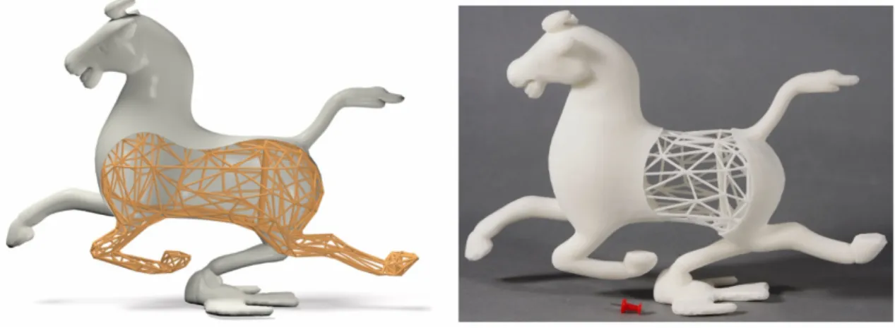
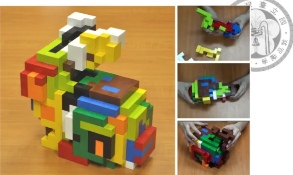
最近因為三維印表機的取得容易許多，使得個人化製造的相關領域受到較多關注，但是一般市面上的三維印表機存在兩個大問題: 需要較長的列印時間以及輸出受限於印表機大小，這些問題使得市售的 3D 印表機無法做到快速大型原型生成，在此研究中，我們提出一個有效率的方法來使用龍圖兒 (Zometool) 做出一個近似原三維模型的結果。

為了要使組裝更容易以及使用更少材料，方法中使用了大區塊的形狀抽象化，輸入的三維模型先以分區法分為許多類似圓柱形的區塊，接著將各區塊的邊界轉為環形的龍圖兒結構，之後再以搜尋最短路徑的方法找尋環形之間的連接結構，最後再順著各分區的軸產生一些中間的環來逼近原三維模型，此論文並附上一些實際拼出的結果圖與分析圖表來展示本研究方法的實用性。

本研究提供一個系統來實現所有論文中提到的演算法，並且加入良好的圖形化使用者介面使的結果有更好的呈現，同時以此介面加速使用者組合實際龍圖兒原型的過程，在最後將會附上系統圖呈現。

關鍵字：龍圖兒結構, 非流形結構, 大型, 原型生成, 模型處理

(6)

Abstract

In recent years, personalized fabrication has attracted much attention due to the greatly improved accessibility of consumer-level 3D printers. However, consumer 3D printers still suffers from the relatively long production time and limited output size, which are undesirable factors to large-scale rapid- prototyping. In this paper, we present an efficient method to approximate a given 3D shape with Zometool.

To achieve ease of assembly and economic usage of building units, the proposed method generates the Zometool structures through a higher level of shape abstraction. The input model is first partitioned into a collection of generalized cylinders by mesh segmentation. The boundaries of mesh segments are converted into ring-like structures and inter-linked by finding the shortest path between them. Additional ring structures are then added along the representative axis of each segment to better approximate the underlying 3D shape. We demonstrate the effectiveness of the proposed method by a variety of 3D models along with examples of the physically fabricated objects.

Key words: Zometool structure, Non-manifold structure, Large-scale, Pro- totyping, Modeling

(7)

List of Figures

3.1 3D printer acceleration of construction by ”Cost-effective Printing of 3D Objects with Skin-Frame Structures”. . . 6 3.2 3D printer acceleration of construction by ”Approximate Pyramidal Shape

Decomposition”. . . 7 3.3 Large-scale construction using 3D printer by ”Chopper: Partitioning Mod-

els into 3D-Printable Parts”. . . 8 3.4 Decreasing supporting structures by ”Approximate Pyramidal Shape De-

composition”. . . 8 3.5 Construction with other material by ”crdbrd: Shape Fabrication by Sliding

Planar Slices”. . . 9 3.6 Construction with other material by ”Making Papercraft Toys from Meshes

Using Strip-based Approximate Unfolding”. . . 9 3.7 Construction with other material by ”Recursive Interlocking Puzzles”. . . 10 3.8 Zometool Shape Approximation. . . 11 3.9 Zometool Rationalization of Freeform Surfaces. . . 11

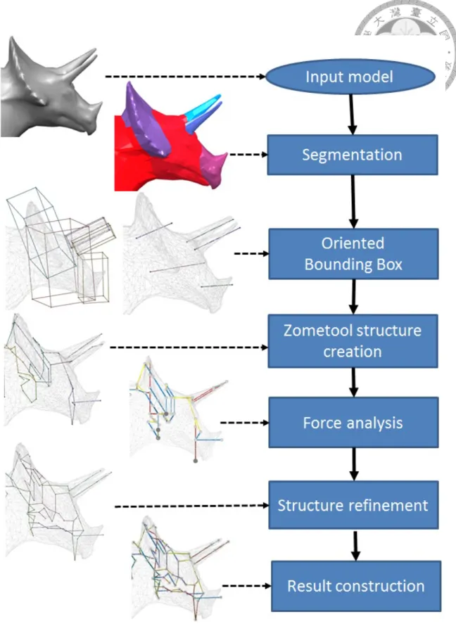
4.1 System overview. Given an input model (a), which is segmented into a collection of sub-parts (b). We compute the oriented bounding box the principal axis of each segment (c) and generate Zometool structures accordingly (d). The system optionally accepts moderate user input to add supporting structures (e). The system visualizes the synthesis result to guide user to build the physical object (f). . . 15

(10)

5.1 The left one is input model , middle one is the result of segmentation, and the right one is the result of oriented bounding box. . . 16 5.2 Ring generation. (a) All points. (b) Delete the points with the distance

less than the length of the shortest strut. (c) Mark next point. (d) Repeat step(b)(c). (e) Get ring. . . 17 5.3 Example of the special axis selection. In the segment, the longest axis

of bounding box(as green arrow) may not be the best axis, and the axis draw (red arrow) in the Figure is the most appropriate. Yellow curve is the cross ring, and its normal vector is red arrow. Because the N_a = 1, we just use the normal vector to be the growing axis ,and not the longest OBB axis(green arrow). . . 18 5.4 Additional features on the model. The yellow rings are interjacent features

and the green point is outward feature. Interjacent features add a ring of struts to fit, and outward features may add a ring or a point according to the end. . . 19 5.5 All close directions. The center hole is the core direction, and columns

from left to right represent the blue, red, and yellow strut as the core direction. The upper row represent layer 1, and the row below is layer 2.

Every step of path searching only get a new direction of strut, in other words, we choose only one strut from all possible directions no matter in layer 1 or layer 2. . . 20 5.6 Demonstration of path connection. (a) Calculate the vector between end

point and start point (V_m), (b) Use V_mto find the closest direction on node (D_m as red arrows) and get the near directions of the D_m (blue arrows).

Each direction has three sizes of struts. (c) Add the best vector to path and loop the step(b). , (d) Get the whole path. The detailed approach is in section 5.2. . . 21

(11)

5.7 Demonstration of Slicing Ring Generation. Yellow curve means the cross ring, and the growing axis is the red arrow. There is a path as green arrows, and we will slice the model to get the interjacent features just like the orange curve. . . 23 5.8 Demonstration of adding support. We have the path and ring as figure 5.7.

Yellow point is the node on the path and the ring, purple arrow is finding the farthest on the same ring, and we get the pink node, so we create a path from the pink node to the closest node on other ring or any node on the structure as brown path. . . 24 5.9 Difference between adding support or not show with Zometool structure.

In the left one, the two rings in the middle only connect with a strut, so it is not stable. After we add the support automatically, the structure is stronger than before in right one. . . 25 5.10 Example of multi-branch segments. In the beginning, we have yellow

rings as cross rings, and we use growing axis to decide the precedence.

Then link the cross rings with path from left to right on the figure as green paths. . . 26 5.11 Three types of the directions about force. Up directions receive the weight

passed from upper structure; Horizontal directions share the weight to horizontal nodes; Down directions pass the weight to the nodes below. . . 27 5.12 Zometool result with gravity analysis. Gray points are weak nodes whose

weight on node are over the threshold. . . 28 5.13 Zometool refined result with gravity analysis. We connect the paths of

one of the weak nodes and analysis again, and the weak point shift to the lower point. It means the weight pass to other nodes successfully. . . 28

6.1 Zometool structure of triceratops. # of Vertex = 2832. # of Edges = 8490.

Segmenting Time = 2.515s. Processing Time = 0.867s. Base # of nodes

= 187. Base # of struts = 213. Refine # of nodes = 610. Refine # of struts

= 679. . . 32

(12)

6.2 Zometool structure of bird. # of Vertex = 3478. # of Edges = 10428.

Segmenting Time = 2.341s. Processing Time = 0.31s. Base # of nodes = 93. Base # of struts = 116. Refine # of nodes = 121. Refine # of struts = 270. . . 33 6.3 Zometool structure of dolphin. # of Vertex = 5216. # of Edges = 15642.

= 420. . . 34 6.4 Zometool structure of octopus. # of Vertex = 5944. # of Edges = 17832.

= 557. . . 35 6.5 Zometool structure of triceratops. # of Vertex = 13826. # of Edges =

41472. Segmenting Time = 9.487s. Processing Time = 1.729s. Base # of nodes = 394. Base # of struts = 434. Refine # of nodes = 831. Refine # of struts = 1385. . . 36 6.6 Zometool structure of ant. # of Vertex = 8299. # of Edges = 24891. Seg-

menting Time = 5.367s. Processing Time = 0.388s. Base # of nodes = 219. Base # of struts = 262. Refine # of nodes = 268. Refine # of struts = 352. . . 37 6.7 Results of vase. Left one is the base result, middle one is the refine result,

and the right one is the real model constructed with Zometool. . . 38 6.8 Result of triceratops. . . 38 6.9 Results of table. In this case, we also use the paper and material to fit the

surface, and the figures shows the constructing steps. . . 39

(13)

7.1 Split windows for result construction. The biggest one shows the whole model, and three right windows show the selected point with different view direction. They are front view, back view, view with the same direction as left window from top to bottom. Besides, there is a log window at bottom to show logs about the vertex information(the edge indices to use) when user click the vertex. . . 41 7.2 Aid for Zometool construction. It shows indices of all directions on the

node. The left node is the front view for the up right window, and the right node is the back view for the middle right window. . . 41 7.3 Screenshot of practical graphical user interface without log window. . . . 42 7.4 Screenshot of practical graphical user interface with log window and black

background. . . 42

8.1 The method to measure bending moment. We tie the dumbbell to the middle of the strut, and ensure that the strut would not contact the chair. . . . 44 8.2 The method to measure shear force. We tie the dumbbell to the strut near

the node, and stop until the situation as figure 8.4 or as figure 8.5. . . 45 8.3 The method to measure friction. We tie the dumbbell to the node and hold

the other side of the strut. We keep increasing the weight until the node dropping. . . 46 8.4 The extreme situation for three types of struts. The color of the middle

part of struts become lighter, and we stop adding force when it happens.

Weight of dumbbell for yellow strut is 3 kilogram; Weight of dumbbell for blue strut is 5 kilogram; Weight of dumbbell for red strut is 4 kilogram. 46 8.5 The tenons after undergoing the extreme situation, and it can be the judge-

ment standards for the structural safety. If the color of tenons are lighter, it is the warning for safety. . . 47

(14)

List of Tables

6.1 Model data and processing results (part 1). . . 31 6.2 Model data and processing results (part 2). Results are measured on a

desktop PC equipped with an Intel i7 3770 3.40GHz CPU. Processing time of ”Zometool Rationalization of Freeform Surfaces” : Model with 5820 faces needs 130 minutes to calculate. . . 31

8.1 All data of measurement results . . . 43

9.1 Table about difference between our system ,3D printer and previous works. 48

(15)

Chapter 1 Motivation

The production cost of 3D printer has been declining and it is available for everyone, so large amount of applications and requirements for fabrication emerge. As a result, fabrication becomes a significant topic. However, the consumer level 3D printers have some drawbacks: 1.the time consuming process 2. the limited output size 3.relatively high cost and not reusable materials 4.need support structure. Large-scale fabrication is needed for some situations. For instances, the props for stage play are usually composed of wooden boards and lack complete 3D structure. In addition, The prototypes for art exhibition are needed when planning in advance. The large-scale prototypes require fast construction and just fit the coarse outline, but recent 3D printers can not realize these features.

The popular modeling system, Zometool, is potentially suitable for providing an al- ternative solution to the scenarios mentioned above. It has several advantages: Firstly, stability, expandability and lightness satisfying the requirements for large-scale fabrication. Secondly, its independent structure and modularity can parallelize the construction to speed up the building process. However, even for 3D models of moderate complexity, novice users may still have difficulty in building visually plausible results by themselves.

Therefore, the goal of this work is to develop an automatic system to assist users to realize Zometool rapid-prototyping with a specified 3D shape.

(16)

Chapter 2 Introduction

Zometool is a tangible, mathematical modeling system not only used in various fields of science for research and teaching, but also recreationally for personal fabrication. It consists of 3 different edge types (or struts) each coming in 3 different lengths related by the golden ratio. The single node type has 62 different slots (or directions) based on 2, 3, and 5-fold symmetry axes. Although being limited in the sense of having only a small, discrete set of available angles and edges, the Zometool system allows for a very rich set of structures.

In this paper, we present a novel technique, which optionally accepts moderate user input, to enables users automatically generate Zometool structures abstract a given 3D input model. The proposed method first performs mesh segmentation to split the complex 3D model into a collection of parts of lower complexity resembling generalized cylinders or cones. The boundaries of segments are primary candidates for the structure of Zometool.

Then, we find the oriented bounding box to match the segment to extract the representative axis for each segment. The representative axis in each segment (named growing axis) have a great influence of constructing Zometool structure, so we implement an algorithm to choose the best axis. It can not only be decided by bounding box, but also by the segment information to judge the best one. The other important factor is obtaining the features. There are two types of features, interjacent ones is in section 5.3 and outward ones in section 5.4.1. These two types come out with different situation about the num-

(17)

ber of segments adjacent to a segment(N_a), and outward features are the special cases of the interjacent features and they will be produced only when N_a = 1. Then we find the Zometool structure with all features. We have two methods for path searching and deal with the balance of approximate solutions and optimized solutions for speed and error.

Recently, several computational schemes have been proposed to accomplish shape approximation with Zometool [1, 2]. In [2], volumetric voxelization is adopted to obtain a rough approximation of the input model, making the method feature-insensitive in nature.

Because the resolution of the regular grid is fixed for the whole model, it is difficult to keep the features and reduce the usage of materials at the same time. [1] uses computation intensive optimization to fit the surface and rebuild the structure when encountering deadlocks. The previous methods generate 2-manifold mesh approximation of the given shape while our method aim to achieve more economic usage of building units with higher level of shape abstraction. So our approach uses non-manifold structures, and thus can present the features directly with less building units. We are not just fitting the surfaces. Our approach just get the obvious features to abstract the original model, and we use the quick method for path searching in most cases unless the start point and end point are fixed, so we can construct the Zometool model in a short time.

There are two primary contributions in this paper: First, our approach use the non- manifold structure to present the model for emphasizing the features, and minimize the amount of building units at the same time. Second, economic usage of Zometool building units give us an edge over the two papers [1,2], and accelerate the construction at the same time.

We have a complete system with great GUI for user, and embed all benefits of this work Third, we creating a complete system for producing Zometool structure. There are straightforward operating steps for users, and the system find out the result automatically with a few inputs by user.

(18)

After the result has been calculated, the system provides a convenient user interface for constructing the Zometool structure using the Zometool in the real world. The GUI accelerate the process of constructing and decrease a lot of toilsome work for finding the right Zometool struts.

(19)

Chapter 3 Related Work

3.1 Mesh Segmentation

Mesh segmentation is an important step for decreasing the complexity of the model by splitting the original model to many small segments, and we prefer to get the parts which have the boundaries cutting at the articulation to get the better results. There are a lot of 3D mesh segmentation algorithms which have been proposed, including K-means [3], graph cuts [4, 5], primitive fitting [6], random walks [7], core extraction [8], spectral clustering [9], critical point analysis [10], shape diameter function [11].

Because we expect the results of segmentation are many general cylinders or cones (the reason is shown in section 5.1), so we select two methods, primitive fitting [6] and shape diameter function [11], and we tried the output of the two method and found that the shape diameter function provides better boundary between segments. The method of primitive fitting [6] loss some important segments, and can only select the number of segments. It can not get the appropriate result by change the parameters, and there are not only primitive shapes on the original model but also some special shapes on the model, but it ignore the large segment with the shape we want to avoid, so primitive fitting can not produce the results we need.

The other work [11] calculate the shape diameter function to get the parts of model

(20)

with the similar diameter, so it can split the segments to cylinders or cones, and the special shape can be separated to some new parts. Just like a moon-like shape, shape diameter function can produce at least two parts to split, but primitive fitting can not find the cylinder on the model part, so it ignore that part and output the original part as output. As a result, we choose the shape diameter function as our implementation of segmentation.

Figure 3.1: 3D printer acceleration of construction by ”Cost-effective Printing of 3D Objects with Skin-Frame Structures”.

3.2 Computational Fabrication

In recent years, computational fabrication has attracted much attention in the reseach fields such as computer graphics and human computer interaction. Some works fabricate functional objects like [12–14]. They can ignore problems on constructing because they have a more important function for the result; some works reduce or change the material to accelerate the process such as [15–18]. [15, 16] use the thin structure to construct the base result like a wireframe and [15] can use the glue to generate the surface.

Our work also generate the structure like wireframe or skeleton to speed up and use the material to encase the result representing the surface. [17] use the mesh joinery to realize the speed up, but the materials of the building units are not popular and that are not available for everyone. That work prove that using other material really speed up the process

(21)

Figure 3.2: 3D printer acceleration of construction by ”Approximate Pyramidal Shape Decomposition”.

and can produce large-scale results, and [18] is like coating a interwoven material on the result of [17].

Large-scale construction is also a problem of 3D printer. Without special treatment, normal 3D printer can only print the results which are smaller than the size of 3D printer, so there are some works try to solve the problem by divide the input model and assemble the parts after printing like [19, 20].

The works using 3D printer would be restricted by the defects of 3D printer, and they encounter the problem of constructive speed and the flexibility to extend or alter the result, so they only produce a small result because of consuming a lot of time on fabrication.

Many works comprehend the constrain of 3d printer, so they choose other materials to construct the result, and we also abandon the normal material and compact structure to pursue the target of large-scale rapid fabrication, and there are large amount of works using other materials, such as [21–23]. Constructing model using other materials has some

(22)

Figure 3.3: Large-scale construction using 3D printer by ”Chopper: Partitioning Models into 3D-Printable Parts”.

Figure 3.4: Decreasing supporting structures by ”Approximate Pyramidal Shape Decom- position”.

benefits: accessible and reusable materials, rapid-constructing, and so on, so we choose the Zometool to be the building units and output sparse results by our method, and we can easily build up a large-scale result, because our approach fits the outward features first and generates the supports later. We can rapidly obtain the basic model to have a roughly prototype to construct with the real building units. If users need a refined and stable result, we can add supports with simple operations. The user just need to provide the points they want to connect, and our approach produce the best Zometool structures.

(23)

Figure 3.5: Construction with other material by ”crdbrd: Shape Fabrication by Sliding Planar Slices”.

Figure 3.6: Construction with other material by ”Making Papercraft Toys from Meshes Using Strip-based Approximate Unfolding”.

3.3 Zometool Design and Modeling

There are two software tools for designing Zometool structures: vZome [24] and ZomeCAD [25], and they are both powerful manual design interface. Their system support adding struts one by one and some different ways to grow the structure by using symmetry or creating substructures, but the users can only build up the result by themselves strut by strut. This is just like build up a real one, and their system just show it on the computer.

Most of the users can not build up the model directly because they do not know if the struts would be linked together after the struts grows apart, so automatic production and optimization are necessary.

[2] use voxelize to get the initial result and process the boundary points and edges on

(24)

Figure 3.7: Construction with other material by ”Recursive Interlocking Puzzles”.

voxel to optimize the result to fit the features on model. This work use local optimization to reduce the processing time by processing small amount of nodes and struts in one oper- ation, and our approach also use local optimization to accelerate, we only use optimization in short distances. When we have to deal with the problem in long distances, we just use the quick approach of direct guess(in section 5.2) to shrink the distance between target points until the distance is appropriate for optimizing. The fatal problem of resolution is mentioned in introduction and we solve it with non-manifold structure.

[1] uses the harmonic field to decide the order of procession, and it can restrict the area of expanding. The harmonic field can reduce the complexity of optimization, but they encounter more deadlocks because of it, so they need more time to refine the result.

Our approach can tolerate a few error to avoid the deadlock, and use segmentation to split the model into many small segments to restrict the area of expanding to speed up the process as that work.

Our approach consider the features first, and then deal with the surfaces. Surfaces are always continuous between the feature points, so after we get the feature points, we

(25)

Figure 3.8: Zometool Shape Approximation.

Figure 3.9: Zometool Rationalization of Freeform Surfaces.

know the surfaces in the same time. Because of finding the features first, we can get a simple result and adjust the compactness by user to decide the amount of building units.

In addition, our structure is non-manifold, so we can present the result directly with less building units. For example, if there is a cone or a needle on the model, we can use just a point to represent the end of cone or needle, and we use the material to cover the result to replace the surface on model. It makes the result looks smoother and be more like an object, furthermore, we can decide the color of the material to make it real.

(26)

3.4 Stability Analysis

There are various methods dealing with the stability analysis, and the calculations about friction are common adopted, including [26–35]. We select a simple friction model for stability analysis to fit our Zometool structure.

(27)

Chapter 4 Overview

There is a flow chart at figure 4.1, and first step is mesh segmentation. User has two parameters to control: cluster level is the number of clusters for the soft clustering and smoothness is a factor which indicates the importance of the surface features for the energy minimization. High smoothness results in a small number of segments, since constructing a segment boundary would be expensive. In other words, merging facets that are placed under different clusters is less expensive than separating them and creating boundaries. We expect the results of segments are cylinder-like or corn-like, because our method will consider the boundaries as rings or points to fit the data structure of non-manifold, and we can obtain the result faster with this assumption. After mesh segmentation has finished, we can get the points which are the boundary of the segment and cross between two segments (named cross points). We order the points to a ring (named cross ring), and the method is shown in section 5.1.1.

Second step is to calculate the oriented bounding box and obtain growing axis for all segments. Growing axis is one of the three axes of the oriented bounding box and it decides the main direction for growing the Zometool structure in each segment. The method for judgement is shown in section 5.1.2. It is important for every segments to own a growing axis, because growing axis decides the main direction to find the features between the boundaries in section 5.3 and can be used to solve the problem about the segments with only one boundary in section 5.4.1.

(28)

In the next step, we need to connect all cross rings and decide the order to execution of the segments with N_a. In a segment, we also decide the execution order with the growing axis by projecting the center points of the cross rings to the growing axis. When we connect the rings, we first connect two points on two rings with the methods in section 5.2, and we also add interjacent features after the path is decided. We create some slices on the nodes on the path with the growing axis as a normal vector, and use the method in section 5.1.1 to create rings of interjacent features.

Up to now we have a lot of rings, but it is not stable enough, so we add the supports to connect the weak structures. There are two steps for adding supports. First step just create basic connection from the weakest node on the rings to other rings to ensure the structure will not be swayed, and the second step connects all probable weak nodes. The method to judge the weakest node on the rings and all probable weak nodes will be mentioned in the section 5.3.3.

Finally, the system transforms the polylines to the Zometool struts, and we provide the convenient user interface for constructing the result. User can look up the struts informations for each node to speed up the process of building up the result.

(29)

Figure 4.1: System overview. Given an input model (a), which is segmented into a collection of sub-parts (b). We compute the oriented bounding box the principal axis of each segment (c) and generate Zometool structures accordingly (d). The system optionally accepts moderate user input to add supporting structures (e). The system visualizes the synthesis result to guide user to build the physical object (f).

(30)

Chapter 5 Zometool Construction

Figure 5.1: The left one is input model , middle one is the result of segmentation, and the right one is the result of oriented bounding box.

5.1 Preprocessing

After the model has loaded, the next step is model segmentation. Users can set cluster level and smoothness parameter to get the segmenting result they want, however, the default value can cover in most instances. System will give a appropriate segmenting result unless the user needs a special output just like excessive number of segments.

(31)

We expect the segmentation results would be general cylinders or cones, and we adopt the shape diameter function [11] to segment the input model, because we will slice the model for getting the rings to compose the features, and general cylinders and cones can easily predict the middle slice and the end. It can decrease the complexity and speed up the process, so it is suitable for rapid fabrication and figure 5.1 shows the input and outputs in this stage.

Figure 5.2: Ring generation. (a) All points. (b) Delete the points with the distance less than the length of the shortest strut. (c) Mark next point. (d) Repeat step(b)(c). (e) Get ring.

5.1.1 Ring Generation

Now we have groups of cross points, and we need orders for the points to create the Zometool structure, so we make the cross rings.

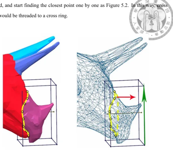
First we delete some points to keep the least distance between any two points. The distance is set the length of the shortest Zometool strut. Then we pick one of them to be

(32)

the head, and start finding the closest point one by one as Figure 5.2. In this way, cross points would be threaded to a cross ring.

Figure 5.3: Example of the special axis selection. In the segment, the longest axis of bounding box(as green arrow) may not be the best axis, and the axis draw (red arrow) in the Figure is the most appropriate. Yellow curve is the cross ring, and its normal vector is red arrow. Because the N_a= 1, we just use the normal vector to be the growing axis ,and not the longest OBB axis(green arrow).

5.1.2 Axis Decision

The segmentation and cross ring generation are complete, and then we calculate the oriented bounding box(OBB) for each segments. Because the process of finding OBB is fast and we just need a approximate solution, so we just use brute-force method to scan all directions with the alternation of 5 degree to get the OBB. There are three axis for each bounding box, but the system needs a main axis to make sure that the system can get the most feature points from the original model for constructing Zometool structure, because if the growing axis has the closest direction to the normal vectors of faces which are made from cross rings, the result of slicing the model would be well-distributed.

(33)

In most cases, the longest axis would be the best axis to choose, but sometimes the longest one is not appropriate as shown in the Figure 5.3. We assume segments to be general cylinders, so we approximate the cross ring with a plane and calculate the normal vector of it. when Na=1, there is only a normal vector of cross ring, we compare the three axis of the OBB, and use the closest axis. when N_a>1, We have to separately count the number of fitting as N_a=1, and if there is only a counter of axis more than two, it means all normal vectors direct the same, so we select that axis; and if there are more than two counters has the number more than two or all counters have the number less than two, it means that the growing axis can not be decide by normal vectors and we just use the longest axis to be the growing axis. LetP be the points on the cross ring, ¯p be the centroid ofP. The normal vector n of the approximate plane of P is obtained by the following equation:

n = ^∑

pi∈P

{ p_i− ¯p

|pi− ¯p| × p_i+1− ¯p

|pi+1− ¯p|

}

. (5.1)

We then calculate the angle between n and the three axes of oriented bounding box. The axis with the minimum value is chosen as the representative axis.

Figure 5.4: Additional features on the model. The yellow rings are interjacent features and the green point is outward feature. Interjacent features add a ring of struts to fit, and outward features may add a ring or a point according to the end.

(34)

5.2 Zometool Path Search

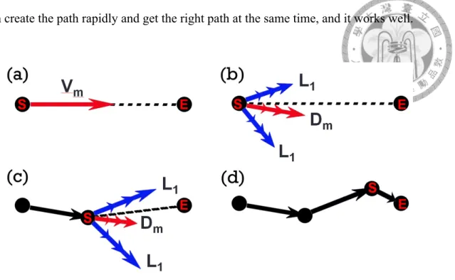
We have a lot of feature points on the model, but it is impossible that the points can be connected directly by Zometool structure, so the system should find out the result to connect any two nodes. The following paragraphs show the methods to connect points using Zometool struts. Both approaches use the vector (V_m) from start point to end point to find the closest direction on the node as the initial guess, and it correspond to a direction (Dm) on node, named core direction.

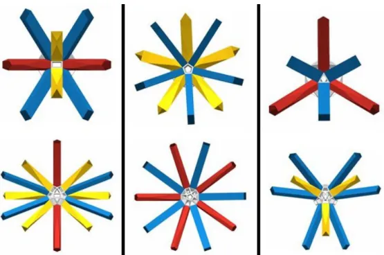
Figure 5.5: All close directions. The center hole is the core direction, and columns from left to right represent the blue, red, and yellow strut as the core direction. The upper row represent layer 1, and the row below is layer 2. Every step of path searching only get a new direction of strut, in other words, we choose only one strut from all possible directions no matter in layer 1 or layer 2.

There are two methods to find the path, the quick approach focuses on the speed and will have more error to the target, so we use this method when the end node is not decided and it has some tolerance to fit the end. The optimized approach is for the situation that the start point and the end point are determined. The optimized approach need more time to find the answer, but it can guarantee that the answer can be found. We prefer to use the quick approach first, and use the optimized approach only when it must be used, so we

(35)

can create the path rapidly and get the right path at the same time, and it works well.

Figure 5.6: Demonstration of path connection. (a) Calculate the vector between end point and start point (V_m), (b) Use V_m to find the closest direction on node (D_mas red arrows) and get the near directions of the D_m (blue arrows). Each direction has three sizes of struts. (c) Add the best vector to path and loop the step(b). , (d) Get the whole path. The detailed approach is in section 5.2.

5.2.1 Quick approach

Test all directions near the D_m and all size of the struts. In figure 5.5 shows the close directions for any direction, and quick approach use both one and two layer directions to find the best place to be close to the end point. Let P_s be the start point, P_e be the end point, D be all directions in two layers according to D_m, L(d, s) be the three lengths of the struts with direction (d) and strut size (s), s is from 0 to 2 corresponding to three size of struts. The best direction and size of strut are decided by the equation below:

d∈D,s∈{0,1,2}min ∥Pe− (Ps+ d∗ L(d, s))∥ (5.2)

Although we brute-force all the possibilities to find the answer, but this approach only run all circumstances once to get the closest position. The above equation is just one step to approach the end point. This method will loop until the path is close enough within the

(36)

threshold, and the following equation shows the stopping inequality:

Pe− (Ps+^∑

i∈V

vi)

< T, (5.3)

where V refers to the vectors in the path, and T is the threshold. This approach may generate more error because it only get the local minimum, but it is enough for the situation which is not care about completely matching to the end point.

5.2.2 Optimized approach

Use A-star algorithm to optimize the result, and the energy is the summation of the path walk though and the distance from the node on the end of path to the end point.

We only use one layer close directions to decrease the amount of calculation, because most of the directions on layer two increase the energy rapidly. The termination criteria is judging that if the distance from the node on the end of path to the end point is less than the threshold(default 1mm) we set. The following equation shows the energy (E) of the A-star:

E = ^∑

i∈V

∥vi∥ + P_e− (Ps+^∑

i∈V

v_i)

. (5.4)

E decides the order to add next path, and the smaller E will be ordered in the front, and the stopping inequality is the same as quick approach but threshold is very close to zero.

Quick approach and optimized approach both can create the Zometool struts between two points, but these two method are quite apart in time consuming, so we mix them to balance the time and error. When the distance between start point and end point is more than the longest struct, we use the quick approach first and run optimized approach on the last part, so we can get a good enough result in a short time.

(37)

5.3 Structure Construction

Now we only have the cross rings, so we connect the rings in this section. In a segment with N_a = 2, the vacancy between cross rings might exist some features on the original model, we call it interjacent features, and the special cases as N_a = 1 and N_a> 2 will be explained in section 5.4. The following three functions construct the structure and fit the interjacent features: path connection, slice ring generation, and support addition, and the detailed descriptions are in the following subsections.

5.3.1 Path Connection

This function connect two points and calculate the path of the Zometool from start point to end point as figure 5.6, and there are two approaches to find the path. The implementation of quick approach and optimized approach are in the section 5.2. After using the approaches above, We obtain intermediate nodes between start point and end point.

Then we use the slice ring generation to fit the surface.

Figure 5.7: Demonstration of Slicing Ring Generation. Yellow curve means the cross ring, and the growing axis is the red arrow. There is a path as green arrows, and we will slice the model to get the interjacent features just like the orange curve.

(38)

5.3.2 Slicing Ring Generation

The figure 5.7 demonstrate it. For fitting the surface, we slice the model with the plane which have the normal vector as growing axis and the nodes of reference are selected on the path which are produced before. We can get the sample points on the segment, and then use the ring generation in section 5.1.1 to string the sample points to a ring. The rings we obtain with this method are interjacent features, and can fit the original model better.

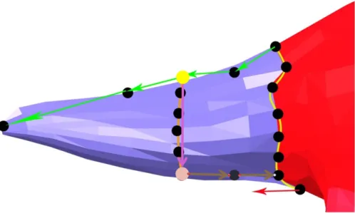
Figure 5.8: Demonstration of adding support. We have the path and ring as figure 5.7.

Yellow point is the node on the path and the ring, purple arrow is finding the farthest on the same ring, and we get the pink node, so we create a path from the pink node to the closest node on other ring or any node on the structure as brown path.

5.3.3 Support Addition

The rings created by previous subsections only connect like a string, but they are not stable because the rings are only connected with one Zometool path. There are two steps to create the supports, the first one only process the weakest nodes on a ring, and the second one analyze the whole structure to find the probable weak nodes to link. We will introduce the two methods Sequentially in the following.

(39)

Figure 5.9: Difference between adding support or not show with Zometool structure. In the left one, the two rings in the middle only connect with a strut, so it is not stable. After we add the support automatically, the structure is stronger than before in right one.

First, as we know, one node on the ring is connected, so we get the farthest node rel- ative to that linked node to find a supporting path to link to the whole Zometool structure by searching the closest node on it. Show in figure 5.8 and figure 5.9.

Second, We have the basic fix structure but it is not strong enough, so we analyze all nodes to find the weaker node with all nodes adjacent to that have only two struts link out.

This method can find the potential weak nodes which are located on a long string, and we can link these nodes to others to make it stable than before.

5.4 Special Cases

5.4.1 Outward Features

Outward feature is a special case of a segment, so we have to change the situation to the normal form. Outward feature is needed when the segment has N_a = 1 and we can produce the outward feature at the end away from the cross ring. Figure 5.4 shows an example. The shape of the segment might be a cylinder or a cone, but our approach can

(40)

deal with these two situation in the same way, because of the non-manifold structure. We first use the growing axis to find the farthest point from the cross ring, and use slice ring generation in section 5.3.2 to get the ring (or a point when the sample points are too close)

at the end. Then use the path connection in section 5.3.1 to connect the end ring and cross ring.

5.4.2 Multi-Branch Segments

The segments of trunk always have N_a > 2 as figure 5.10, so we need a method to find the order to link the cross rings. We first calculate the center point of the cross rings, and use it to decide the precedence with growing axis. Then, we can link the cross rings with path one by one, and this situation is the same as Na= 2.

Figure 5.10: Example of multi-branch segments. In the beginning, we have yellow rings as cross rings, and we use growing axis to decide the precedence. Then link the cross rings with path from left to right on the figure as green paths.

5.5 Gravity Analysis

We calculate the weight and normal force from top to the bottom, and the normal force will pass the weight in the process, so usually the nodes below bear more weight and normal force, but sometimes will distribute to more nodes to bear, as a result, each node bear

(41)

part of the weight from the upper node.

Figure 5.11: Three types of the directions about force. Up directions receive the weight passed from upper structure; Horizontal directions share the weight to horizontal nodes;

Down directions pass the weight to the nodes below.

5.5.1 Method Implement

We first define three types of directions: up, horizontal, and down directions as figure 5.11. First, initialize the weight on each node as weight of node. Then we process the nodes by the order of height from high to low. For each node, we add the weight on upper node and struts to the processing node with following equation:

Wprocessing(new) = Wprocessing(old)+ ^∑

all upper struts

( W_{upper node} Ndown struts of upper node

+ W_strut) (5.5) W means weight and N means amount number. Besides the equation, we find all nodes connect with horizontal struts and share the weight before the height of processing node changes. The method to share the weight is split the weight into (Nhorizontal struts+ 1) parts and pass the weights to horizontal nodes.

(42)

With this method and we set a threshold, we can find the weak points, and we show the weak point on the model. we can create paths on the weak nodes by linked to other nodes or can just show the weak nodes and let user to select the nodes to link, and then we get a stronger structure.

Figure 5.12: Zometool result with gravity analysis. Gray points are weak nodes whose weight on node are over the threshold.

Figure 5.13: Zometool refined result with gravity analysis. We connect the paths of one of the weak nodes and analysis again, and the weak point shift to the lower point. It means the weight pass to other nodes successfully.

(43)

Chapter 6 Results and Discussion

In this section, we demonstrate the results of our system on a number of examples.

Our system automatically generate the base result, and we provide the function for user to refine the output. The base result guarantee the connectivity and the basic stability. If the users need a stabler result, they just need to find out pairs of points they want to connect, and the system will automatically create the path for Zometool structure.

We choose the Computational Geometry Algorithms Library (CGAL) to deal with the segmentation. The package of triangulated surface mesh segmentation in CGAL provides an implementation of the algorithm relying on the shape diameter function [11].

The data of the Zometool struts and nodes are set by the real size, and there are some important parameters:

1. Minimum diameter of a ring is set to be the shortest strut plus the diameter of node, because if the diameter of a ring is smaller than the smallest strut, it does not exist the structure to construct a ring, and it judges the whether the ring should be shrink to a point.

2. Minimum size of connect two points is the same as the minimum diameter of a ring because the shortest strut is the same, and it is the condition to know if two points has a strut to connect.

(44)

3. Maximum size of connect two points is set to be the longest strut plus the diameter of node, and it is ised to judge to be the boundary to use the quick approach or optimize approach.

4. Optimized threshold is set to be 0.3cm for the Zometool has a few flexibility to tolerate this error in our non-manifold structure.

6.1 Performance

The descriptions in result figures show the model information used in this paper and the performance measured on a desktop PC equipped with an Intel i7 3770 3.40GHz CPU and 20GB RAM. The optimization time is proportional to the number of vertices,and it usually takes only seconds to obtain the result.

6.2 Limitation and future work

The proposed still has several limitations. First, it sometimes cannot find the most appropriate growing axis when local mesh vertices are isotropically distributed and the orientation check is ambiguous. In this case, we simply select the longest axis of the OBB.

Second, our approach mainly deal with the connectivity and feature maintenance, and we provide semi-automatic structural supports to enhance the stability. It can be a future work to consider the structure stability, and generate results of different fineness to give users to select the sparse or complex result they needs.

6.3 Results

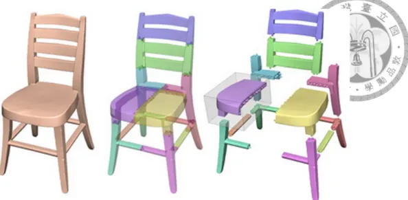
The followings figure 6.1 to figure 6.5 are the results of the work. There are four pictures that each picture individually means the original models, segmentation result,

(45)

base results, and the refined results by user.

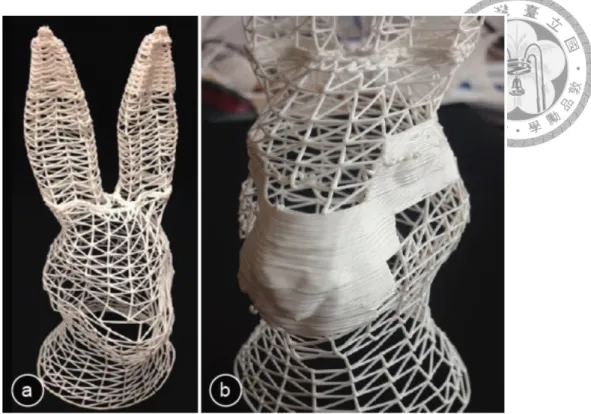
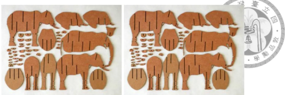
After we construct the Zometool model in real world, we will use paper to produce the surface of the result, and use material to design the pattern of the model just like figure 6.9. In this case, we use A4 paper to coat the Zometool and use pure colour material. If the result need multiple colors, different color patches of materials are usable.

model triceratops bird dolphin octopus

# of Vertex 2832 3478 5216 5944

# of Edges 8490 10428 15642 17832

# of Faces 5660 6952 14238 11888

Segmenting Time 2.468s 2.338s 3.171s 4.044s

Processing Time 5.84s 0.22s 0.342s 0.514s

Add Support Time 5.016s 0.044s 1.52s 4.371s

Force Analysis Time 0.057s 0.038s 0.053s 0.047s

node 610 121 223 171

strut 679 270 420 557

size(cm) 100x43x30 68x12x101 97x30x32 99x73x30 Table 6.1: Model data and processing results (part 1).

model teddy ant vase table

# of Vertex 13826 8299 9299 6626

# of Edges 41472 24891 27891 19872

# of Faces 27648 16594 18594 13248

Segmenting Time 9.16s 5.367s 10.577s 4.379s

Processing Time 0.423s 0.388s 0.41s 4.502s

Add Support Time 0.924s 0.307s 10.017s 4.553s Force Analysis Time 0.077s 0.001s 0.077s 0.001s

node 831 268 601 430

strut 1385 352 675 538

size(cm) 80x96x38 63x97x54 44x93x45 50x50x18

Table 6.2: Model data and processing results (part 2). Results are measured on a desktop PC equipped with an Intel i7 3770 3.40GHz CPU. Processing time of ”Zometool Ratio- nalization of Freeform Surfaces” : Model with 5820 faces needs 130 minutes to calculate.

(46)

Figure 6.1: Zometool structure of triceratops. # of Vertex = 2832. # of Edges = 8490.

Segmenting Time = 2.515s. Processing Time = 0.867s. Base # of nodes = 187. Base # of struts = 213. Refine # of nodes = 610. Refine # of struts = 679.

(47)

Figure 6.2: Zometool structure of bird. # of Vertex = 3478. # of Edges = 10428. Seg- menting Time = 2.341s. Processing Time = 0.31s. Base # of nodes = 93. Base # of struts

= 116. Refine # of nodes = 121. Refine # of struts = 270.

(48)

Figure 6.3: Zometool structure of dolphin. # of Vertex = 5216. # of Edges = 15642.

(49)

Figure 6.4: Zometool structure of octopus. # of Vertex = 5944. # of Edges = 17832.

(50)

Figure 6.5: Zometool structure of triceratops. # of Vertex = 13826. # of Edges = 41472.

(51)

Figure 6.6: Zometool structure of ant. # of Vertex = 8299. # of Edges = 24891. Segment- ing Time = 5.367s. Processing Time = 0.388s. Base # of nodes = 219. Base # of struts = 262. Refine # of nodes = 268. Refine # of struts = 352.

(52)

Figure 6.7: Results of vase. Left one is the base result, middle one is the refine result, and the right one is the real model constructed with Zometool.

Figure 6.8: Result of triceratops.

(53)

Figure 6.9: Results of table. In this case, we also use the paper and material to fit the surface, and the figures shows the constructing steps.

(54)

Chapter 7 Implementation of System

7.1 System environment

All functions are implemented as a plugin attaching on the Openflipper. Openflip- per is a stable platform to develop the functions. Although it provide a little functions

for mesh processing, it render the results well and has a great Graphical user interface for developer to add plugin and for user to use.

For segmentation, we choose the Computational Geometry Algorithms Library(CGAL) which implements the shape diameter function(SDF) as the default method of segmentation.

7.2 GUI design

The system shows the result with four split windows as Figure 7.1. Different views collocate with the log window and the Figure 7.2 to speed up the Zometool construction.

The system transforms the polylines to the Zometool struts, and we provide the convenient user interface for constructing the result. User can look up the struts informations for each node to speed up the process of building up the result.

(55)

Figure 7.1: Split windows for result construction. The biggest one shows the whole model, and three right windows show the selected point with different view direction.

They are front view, back view, view with the same direction as left window from top to bottom. Besides, there is a log window at bottom to show logs about the vertex information(the edge indices to use) when user click the vertex.

Figure 7.2: Aid for Zometool construction. It shows indices of all directions on the node.

The left node is the front view for the up right window, and the right node is the back view for the middle right window.

(56)

Figure 7.3: Screenshot of practical graphical user interface without log window.

Figure 7.4: Screenshot of practical graphical user interface with log window and black background.

(57)

Chapter 8 Experiment

For supporting the physical analysis system, we measure some physical parameters.

We measure the bending moment, shear force, and friction.

Bending moment is about the tolerance of bending, and the measuring method is show in figure 8.1. There are two methods to judge the safety as figure 8.4 and figure 8.5.

Shear force represents the force which tenons can bear, so we try to add force on the strut near the node and perpendicular to the direction of strut. Figure 8.2 shows it and figure 8.5 is the stopping condition.

Friction is the resistance force to stabilize the tenons and mortises, and the measuring method is show in figure 8.3.

Yellow/Triangle Blue/Rectangle Red/Pentagon

bending moment 9.4kg•cm 18.3kg•cm 13.9kg•cm

shear force 7kg 9kg 9kg

friction 1kg 1.5kg 2kg

Table 8.1: All data of measurement results

(58)

Figure 8.1: The method to measure bending moment. We tie the dumbbell to the middle of the strut, and ensure that the strut would not contact the chair.

(59)

Figure 8.2: The method to measure shear force. We tie the dumbbell to the strut near the node, and stop until the situation as figure 8.4 or as figure 8.5.

(60)

Figure 8.3: The method to measure friction. We tie the dumbbell to the node and hold the other side of the strut. We keep increasing the weight until the node dropping.

Figure 8.4: The extreme situation for three types of struts. The color of the middle part of struts become lighter, and we stop adding force when it happens. Weight of dumbbell for yellow strut is 3 kilogram; Weight of dumbbell for blue strut is 5 kilogram; Weight of dumbbell for red strut is 4 kilogram.

(61)

Figure 8.5: The tenons after undergoing the extreme situation, and it can be the judgement standards for the structural safety. If the color of tenons are lighter, it is the warning for safety.

(62)

Chapter 9 Conclusion

We have presented an system for large-scale rapid-prototyping that enables users to semi-automatically generate a Zometool structure with a 3D model input. The main prop- erty of the approach is non-manifold based structure to rapidly fit the features and decrease the amount of building units in the same time. In contrast to the previous works about Zometool, we can use less building units to construct the model in the same size, because of our sparse structure, so we can also build up the result faster. And we provide a convenient GUI for user to speed up the process of construct the result. The proposed technique can be use as the large prototype in exhibition, the the props for stage play, and all situations which need the prototype constructed rapidly.

3D Printer TVCG GMOD Ours

Unlimited output size X O O O

Reusable X O O O

Save constructing time X

(2d)

△ (3h)

O (1h)

Save materials X △ △ O

Save processing time - △

(2h)

O (2m)

O (15s)

Must have solution - X O O

Feature preserving in low resolution - △ X O

Can output different size - △ △ O

Table 9.1: Table about difference between our system, 3D printer and previous works.

(63)

Bibliography

[1] H. Zimmer and L. Kobbelt. Zometool rationalization of freeform surfaces. IEEE Trans. Vis. Comput. Graph., 20(10):1461–1473, 2014.

[2] Henrik Zimmer, Florent Lafarge, Pierre Alliez, and Leif Kobbelt. Zometool shape approximation. Graph. Models, 76(5):390–401, 2014.

[3] Shymon Shlafman, Ayellet Tal, and Sagi Katz. Metamorphosis of polyhedral sur- faces using decomposition. Comput. Graph. Forum, 21(3):219–228, 2002.

[4] Aleksey Golovinskiy and Thomas Funkhouser. Randomized cuts for 3D mesh anal- ysis. ACM Trans. Graph., 27(5):145:1–145:12, 2008.

[5] Sagi Katz and Ayellet Tal. Hierarchical mesh decomposition using fuzzy clustering and cuts. ACM Trans. Graph., 22(3):954–961, 2003.

[6] Marco Attene, Bianca Falcidieno, and Michela Spagnuolo. Hierarchical mesh seg- mentation based on fitting primitives. Vis. Comput., 22(3):181–193, 2006.

[7] Yu-Kun Lai, Shi-Min Hu, Ralph R. Martin, and Paul L. Rosin. Fast mesh segmen- tation using random walks. In Proc. SPM ’08, pages 183–191, 2008.

[8] Sagi Katz, George Leifman, and Ayellet Tal. Mesh segmentation using feature point and core extraction. Vis. Comput., 21(8-10):649–658, 2005.

[9] Rong Liu and Hao Zhang. Segmentation of 3D meshes through spectral clustering.

In Proc. PG ’04, pages 298–305, 2004.

(64)

[10] Hsueh-Yi Lin, H. Y. M. Liao, and Ja-Chen. Lin. Visual salience-guided mesh de- composition. IEEE Trans. Multi., 9(1):46–57, 2007.

[11] Lior Shapira, Ariel Shamir, and Daniel Cohen-Or. Consistent mesh partitioning and skeletonisation using the shape diameter function. Vis. Comput., 24(4):249–259, 2008.

[12] Stefanie Mueller, Tobias Mohr, Kerstin Guenther, Johannes Frohnhofen, and Patrick Baudisch. fabrickation: Fast 3D printing of functional objects by integrating con- struction kit building blocks. In Proc. ACM CHI ’14, pages 3827–3834, 2014.

[13] Valkyrie Savage, Colin Chang, and Björn Hartmann. Sauron: Embedded single- camera sensing of printed physical user interfaces. In Proc. ACM UIST ’13, pages 447–456, 2013.

[14] Stefanie Mueller, Pedro Lopes, and Patrick Baudisch. Interactive construction: Inter- active fabrication of functional mechanical devices. In Proc. ACM UIST ’12, pages 599–606, 2012.

[15] Stefanie Mueller, Sangha Im, Serafima Gurevich, Alexander Teibrich, Lisa Pfisterer, François Guimbretière, and Patrick Baudisch. Wireprint: 3D printed previews for fast prototyping. In Proc. ACM UIST ’14, pages 273–280, 2014.

[16] Weiming Wang, Tuanfeng Y. Wang, Zhouwang Yang, Ligang Liu, Xin Tong, Weihua Tong, Jiansong Deng, Falai Chen, and Xiuping Liu. Cost-effective printing of 3D objects with skin-frame structures. ACM Trans. Graph., 32(6):177:1–177:10, 2013.

[17] Paolo Cignoni, Nico Pietroni, Luigi Malomo, and Roberto Scopigno. Field-aligned mesh joinery. ACM Trans. Graph., 33(1):11:1–11:12, 2014.

[18] Akash Garg, Andrew O. Sageman-Furnas, Bailin Deng, Yonghao Yue, Eitan Grin- spun, Mark Pauly, and Max Wardetzky. Wire mesh design. ACM Trans. Graph., 33(4):66:1–66:12, 2014.

(65)

[19] Linjie Luo, Ilya Baran, Szymon Rusinkiewicz, and Wojciech Matusik. Chopper:

partitioning models into 3d-printable parts. ACM Trans. Graph., 31(6):129, 2012.

[20] Ruizhen Hu, Honghua Li, Hao Zhang, and Daniel Cohen-Or. Approximate pyrami- dal shape decomposition. ACM Transactions on Graphics (TOG), 33(6):213, 2014.

[21] Jun Mitani and Hiromasa Suzuki. Making papercraft toys from meshes using strip- based approximate unfolding. ACM Trans. Graph., 23(3):259–263, August 2004.

[22] Kristian Hildebrand, Bernd Bickel, and Marc Alexa. crdbrd: Shape fabrication by sliding planar slices. Computer Graphics Forum, 31(2pt3):583–592, 2012.

[23] Peng Song, Chi-Wing Fu, and Daniel Cohen-Or. Recursive interlocking puzzles.

ACM Trans. Graph., 31(6):128:1–128:10, November 2012.

[24] S. Vorthmann. vZome [online].

[25] E. Schlapp. ZomeCAD. [online].

[26] David Baraff. Fast contact force computation for nonpenetrating rigid bodies. In Proceedings of the 21st Annual Conference on Computer Graphics and Interactive Techniques, SIGGRAPH ’94, pages 23–34, New York, NY, USA, 1994. ACM.

[27] Danny M. Kaufman, Timothy Edmunds, and Dinesh K. Pai. Fast frictional dynamics for rigid bodies. ACM Trans. Graph., 24(3):946–956, July 2005.

[28] D. E. STEWART and J. C. TRINKLE. An implicit time-stepping scheme for rigid body dynamics with inelastic collisions and coulomb friction. International Journal for Numerical Methods in Engineering, 39(15):2673–2691, 1996.

[29] Jong-Shi Pang and David E. Stewart. A unified approach to discrete frictional contact problems. International Journal of Engineering Science, 37(13):1747 – 1768, 1999.

[30] M. Raous, L. Cangémi, and M. Cocu. A consistent model coupling adhesion, friction, and unilateral contact. Computer Methods in Applied Mechanics and Engineering, 177(3–4):383 – 399, 1999.

(66)

[31] Eran Guendelman, Robert Bridson, and Ronald Fedkiw. Nonconvex rigid bodies with stacking. ACM Trans. Graph., 22(3):871–878, July 2003.

[32] Kenny Erleben. Velocity-based shock propagation for multibody dynamics anima- tion. ACM Trans. Graph., 26(2), June 2007.

[33] Danny M. Kaufman, Shinjiro Sueda, Doug L. James, and Dinesh K. Pai. Staggered projections for frictional contact in multibody systems. ACM Trans. Graph., 27(5):

164:1–164:11, December 2008.

[34] Jorge Gascón, Javier S. Zurdo, and Miguel A. Otaduy. Constraint-based simulation of adhesive contact. In Proceedings of the 2010 ACM SIGGRAPH/Eurographics Symposium on Computer Animation, SCA ’10, pages 39–44, Aire-la-Ville, Switzer- land, Switzerland, 2010. Eurographics Association.

[35] Nobuyuki Umetani, Takeo Igarashi, and Niloy J Mitra. Guided exploration of phys- ically valid shapes for furniture design. ACM Trans. Graph., 31(4):86, 2012.