國 立 交 通 大 學
光 電 工 程 研 究 所
碩士論文
非同步約分諧波鎖模掺鉺光纖光固子雷射
之研究
Study of asynchronous rational harmonic
mode-locked Er-doped fiber soliton laser
研 究 生 : 張家豪
指導教授: 賴暎杰
非同步約分諧波鎖模掺鉺光纖光固子雷射
之研究
研究生:張家豪 教授:賴暎杰 老師
國立交通大學光電工程研究所
摘要
非同步鎖模光纖光固子雷射在實驗以及理論上有相當多的研
究及發展,它的許多特性,例如:脈衝的慢速週期性變化、提高
超模的抑制比以及可形成超短且超高重複率的脈衝等,這些在高
速光通訊與超快光學等的應用上都有很好的潛在價值。
在許多提高脈衝重複率的主動諧波鎖模掺鉺光纖雷射之研究
裏脈衝重複率會受限於電子儀器上之限制,利用約分諧波鎖模的
機制可以來產生更高的脈衝序列重複率,但也會造成脈衝序列的
不等高性。在文獻上解決的方法都必須利用其他的元件和機制來
改善,而本論文則是藉由非同步鎖模機制來改善脈衝序列的振幅
不等高性並同時有效地抑制超模噪音(supermode noise),而不
必像文獻上其他方法需依賴其他元件,此外脈衝寬度更可以輕易
地小於 1 psec,這也是目前其他約分諧波鎖模雷射所較難達到
的成效。
Study of asynchronous rational harmonic
mode-locked Er-doped fiber soliton laser
Student:Chia-Hao Chang Advisor:Prof.Yinchieh Lai
Department of Photonics & Institute of Electro-Optical Engineering College of Electrical Engineering and Computer Science National
Chiao-Tung University
Abstract
Active harmonic mode-locked fiber lasers for high repetition rate optical pulse train generation will be limited by the electronic instrument speed. Rational harmonic mode-locking can further increase the pulse repetition rate but the pulse amplitude may not be perfectly equal. In the previous work additional components and mechanisms have to be used for achieving pulse equalization. In this thesis, by developing the new asynchronous rational harmonic mode-locking technique we not only improve the amplitude equalization of the pulse train well but also suppress the supermode noises effectively. Moreover, the achieved pulse-width can be easily shorter than one pico-second. This is one goal that other rational mode-locked fiber lasers couldn't achieve as yet.
誌謝
碩士短短的兩年中,不管是在課業上或是實驗室的研究上都讓我學習到 很多不同的專業知識,尤其在碩士的研究裡,每當遇到瓶頸,賴老師的幾 句話總可以點醒我並且引導我到正確的方向,賴老師也總是不厭其煩地教 導著,讓我可以順利地完成工作並且達到理想的目標。 此外能夠順利的完成研究也必須感謝陳智弘老師、鄒志偉老師等實驗室 大方的贊助儀器,讓我的實驗可以順利的完成。除了陳老師及鄒老師還要 特別感謝彭朋群老師從外校撥空前來擔任口委並且給於我許多寶貴的建 議,這在我往後的學習生涯中有著莫大的幫助。 在賴老師的實驗室裡最讓人感到開心的就是有著學長姐們的關心以及 教導,學長姐們從不會吝嗇用他們的時間來指導我,特別感謝項維巍學長 在實驗上的指導、徐桂珠學姊多方面的幫助以及鞠曉山學長細心的教導, 另外還有林家弘、郭立強學長、許宜蘘學姊以及翁俊仁學長們提供在人生 道路上寶貴的經驗以及完善的建議,讓我以後不管是在研究領域上或是工 作事業裡都可以有信心及能力去解決問題。 最後要感謝實驗室的同學 昱勳、子翔、佩芳、秀鳳、柏萱、柏崴陪伴 我度過這漫長的兩年,彼此的互相勉勵關心,讓實驗室充滿許多歡樂。另 外學弟妹 姿媛、聖閔、力行也讓實驗室帶來年輕的活力和朝氣。 最重要的是要感謝父母以及家人的支持,讓我可以在人生的道路裡順順 利利地完成這一項成就。Contents
Chinese Abstract...I
English Abstract...II
Acknowledgements...III
Contents...IV
List of Figures...VI
Chapter 1: Introduction
1.1 Overview...11.2 Motivation of the research...3
1.3 Organization of the thesis...3
References...4
Chapter 2: Theories of mode-locked fiber lasers
2.1 Active mode-locking...62.1.1 Amplitude modulation mode-locking...7
2.1.2 Phase modulation mode-locking...10
2.2 Rational harmonic mode-locking...12
2.3 Asynchronous harmonic mode-locking...15
2.4 The hybrid harmonic mode-locking...18
Chapter 3: Experimental setup and results
3.1 Experimental setup...23 3.2 Rational harmonic mode-locking results...25 3.3 Asynchronous rational harmonic mode-locking results...33
Chapter 4: Simulations
4.1 Master equation and variational analyses...41
4.2 Simulation results of rational harmonic mode-locking....44 4.3 Simulation results of asynchronous rational harmonic
mode-locking...45 References...47
Chapter 5: Conclusions
5.1 Summary of achievements...48 5.2 Future work...50
List of Figures
Fig.2.1 Schematic of an active mode-locked laser...6
Fig.2.2 Actively mode-locked pulses in the time domain...7
Fig.2.3 Actively mode-locked modes in the frequency domain...8
Fig.2.4 Sketch of the amplitude modulation mode-locking in the frequency domain...9
Fig.2.5 Sketch of phase modulation mode-locking in the time domain...11
Fig.2.6 Formulation of pulse train in the time domain...11
Fig.2.7 Time domain picture of conventional rational harmonic mode locking...14
Fig.2.8 Schematic diagram of asynchronous Laser cavity...15
Fig.2.9 The noise-cleanup effect in the asynchronous soliton mode-locked laser...16
Fig.3.1 The experimental setup...23
Fig.3.2 Electronic spectrum from the microwave synthesizer...26
Fig.3.3 Electronic spectrum after the power amplified...26
Fig.3.4 P=2, 4GHz pulse trains in the RF spectrum...27
Fig.3.5 P=3, 6GHz pulse trains in the RF spectrum...28
Fig.3.6 P=4, 8GHz pulse trains in the RF spectrum...28
Fig.3.7 P=2, 4GHz pulse trains in the fast sampling oscilloscope...29
Fig.3.8 P=3, 6GHz pulse trains in the fast sampling oscilloscope...29
Fig.3.9 P=4, 8GHz pulse trains in the fast sampling oscilloscope...29
Fig.3.10 P=2, 8GHz pulse trains in the RF spectrum...30
Fig.3.11 P=3, 12GHz pulse trains in the RF spectrum...31
Fig.3.14 P=3, 6GHz pulse trains in the RF spectrum...34
Fig.3.15 P=3, 6GHz pulse trains in the fast sampling oscilloscope...34
Fig.3.16 The optical spectrum of the laser output...35
Fig.3.17 P=3, 12GHz pulse trains in the RF spectrum...36
Fig.3.18 The optical spectrum of the laser output...37
Fig.3.19 SHG intensity autocorrelation trace (solid curve) and the fitting curve(open circles) of the laser output, assuming sech2 pulse shape...38
Fig.3.20 P=3, 21GHz pulse trains in the RF spectrum...39
Fig.3.21 The optical spectrum of the laser output...40
Fig.3.22 SHG intensity autocorrelation trace (solid curve) and the fitting curve (open circles) of the laser output, assuming sech2 pulse shape...40
Fig.4.1 Simulation results of RHML evolution equations...44
Fig.4.2 Simulation results of ARHML evolution equations...44
Chapter 1
Introduction
1.1 Overview
Today optical communication has been the main broadband wire
communication science and technology. In optical communication systems, the signals propagate inside the fibers, which is different from wireless communication or traditional cable communication. The optical fibers are less affected by the external factors in comparison to electric cables. They have advantageous characteristics like higher security, low loss, small volume, light weight, and not influenced by electromagnetic waves. Therefore the optical fibers have been widely used in today’s practical networks.
Different kinds of light sources are needed for different fiber communication applications. Semiconductor laser source have been mostly used due to their electrical pumping characteristics, low cost, and compact volume. However, for generating very short optical pulses, the characteristics of modelocked semiconductor lasers are in general not the best due to the large chirp caused by the semiconductor gain dynamics. On the contrary the atomic lifetime of the fiber gain medium is longer than that in the semiconductor laser gain medium. The coupling between the gain and the refractive index is also much less. Therefore in general modelocked fiber lasers can have better pulse quality in comparison to modelocked semiconductor lasers, not to mention that the output power
optical fiber systems. Based on the above consideration the mode-locked fiber laser source research has been very popular in the development of present optical fiber communication technologies.
The method of locking the multiple axial modes in a laser cavity is called mode-locking. Typically we have two popular ways to achieve mode-locking. Active mode-locking can generate pulse trains at higher repetition rates when compared with passive mode-locking. On the other hand, passive mode-locking can generate shorter pulses when compared to active mode-locking. However to generate shorter pulses at high repetition rates simultaneously, hybrid mode-locking can be used by employing the two methods together.
In the past literature many methods have been used to generate the pulse trains of high repetition rates. The common method is the harmonic mode-locking technique. This technique was first introduced and analyzed by Becker et al. by employing frequency modulation [1.1]. Nevertheless, the approach is easily limited by the instrument bandwidth when the pulse trains are operated at very high repetition rates. To break this limitation, the rational harmonic mode-locking technique has been developed [1.2]. By this special method the repetition rate of the pulse trains can be increased by several times, not restricted to the instrument bandwidth, even though there are some issues needed to be solved. The pulse amplitude un-equalization problem is one of them [1.3] and the supermode noise problem is another [1.4].
In recent years the asynchronous harmonic mode-locking technique has been developed [1.5]. Due to the optical carrier frequency sweeping effects caused by asynchronous phase modulation, the noises will be shifted away and the solitons can resist this frequency shift more. Finally, the noises are filtered out by the filter while the solitons can still exist. This noise clean-up effect is similar to the sliding frequency guiding filter effects in soliton transmission systems and can help stabilize the modelocked laser operation. However, it has not been known whether the asynchronous rational harmonic mode-locking can also be realized for operating the laser at an even higher repetition rate.
1.2 Motivation of the research
Harmonic active mode-locking has proven to be a very effective technique for the generation of high-repetition-rate short pulses from fiber lasers. The repetition rate of the output pulses from active mode-locked lasers equals the frequency at which the modulation is performed and is therefore practically limited by the highest operating frequency of the modulator. To overcome these drawbacks, the rational harmonic mode locking (RHML) has been investigated to generate higher repetition rate pulses by using lower frequency synthesizers. However, the higher-order RHML will consequentially lead to an output pulse train of un-equal peak amplitudes. We expect the asynchronous harmonic mode-locking technique we developed previously can be generalized to improve this problem. Therefore in this thesis work we investigate the asynchronous rational harmonic mode locking (ARHML) technique both experimentally and theoretically to demonstrate the feasibility.
1.3 Organization of the thesis
This thesis consists of four chapters. Chapter 1 is an overview of
modelocked fiber lasers and the motivation of this research. Chapter 2 describes the principles of different mode-locking techniques. Chapter 3 shows our experimental setup and the obtained results. In Chapter 4 we also verify the results by theoretical simulation based on variational analysis. Finally, Chapter 5 gives a summary about our completed achievements and future expectations.
R
R
R
e
e
e
f
f
f
e
e
e
r
r
r
e
e
e
n
n
n
c
c
c
e
e
e
[1.1] M. Becker et al., “Harmonic mode locking of the Nd:YAG laser”, IEEE J. Quantum Electron. 8 (8), 687, 1972
[1.2] E. Yoshida and M. Nakazawa, “80–200 GHz erbium doped fiber laser using a rational harmonic mode-locking technique,” Electron. Lett., vol.32, no. 15, pp. 1370–1372, 1996.
[1.3] S. Ozharar, S. Gee, F. Quinlan, S. Lee, and P. J. Delfyett, “Pulse-amplitude equalization by negative impulse modulation for rational harmonic mode-locking,” Opt. Lett. 31, 2924-2926,2005. [1.4] N. Onodera, “Supermode beat suppression in harmonically
mode-locked erbium-doped fiber ring lasers with composite cavity structure,” Electron.Lett., vol. 33, pp. 962–963, May 1997.
[1.5] W.-W Hsiang, C.-Y Lin, M.-F Tien, and Y. Lai, “Direct generation of a 10 GHz 816 fs pulse train from an erbium-fiber soliton laser with asynchronous phase modulation,” Opt. Lett. 30, 2493-2495, 2005.
Chapter 2
Theories of mode-locked fiber lasers
2.1 Active mode-locking
Fig. 2.1 Schematic of an active mode-locked laser.
Active mode-locking involves the periodic modulation of the resonator losses or the round-trip phase change. This can be achieved with an acousto-optic or electro-optic modulator. For high repetition modelocked fiber lasers, it is usually a Mach-Zehnder integrated-optics waveguide-type modulator. If the modulation is synchronized with the resonator round trip time, the intra-cavity optical pulses in synchronization with the modulation can continue to grow and eventually mode-locking is achieved.
Typically, active mode-locked lasers can employ two general methods
of modulation for achieving modelocking. One is the amplitude modulation (AM) mode-locking and the other is the phase modulation (PM) mode-locking. A detailed introduction for the two general methods of modulation will be given in the following sections.
2.1.1 Amplitude modulation mode-locking
Amplitude modulation mode-locking is a method to produce a short
pulse train by modulating directly the optical amplitude of the light. It can be analyzed both in the time and frequency domains [2.1].
In the time domain, the modulation provides a time dependent loss.
Whenever the loss dips below the gain level, net gain is obtained and the curvature of the gain envelope is negative. The optical pulses seen the gain window will continue to grow and get shorten through the gain shaping. However, shorter pulses will experience lager dispersion and thus in the end, the two forces balance each other to form the steady state pulse shape. The modulation time period must be equal to a multiple of the roundtrip time for stable pulses to be generated. Fiqure2.2 shows the active mode-locking process in the time domain.
Fig. 2.2 Actively mode-locked pulses in the time domain and the time dependence of the net gain.
The master equation for modeling the laser can be expressed as, R 1 2 M g a T t g T g l a T t a T t M t a T t T Ω t Ω 2 2 2 2 ( , ) ( ) ( , ) ( , ) ( , ) ∂ = − + ∂ − ∂ ∂ (2.1)
In the frequency domain, as the gain level is above threshold, then the axial modes that see net gain will begin to lase. If the laser is mode-locked by an amplitude modulator, a sinusoidal modulation of the central mode at the frequency ΩM=ΔΩ produces sidebands at ω0±ΩM. We
denote the frequency of the central mode by ω0. These sidebands can
injection-lock the neighboring modes sequentially and the mode-locking is formed eventually. Figure 2.3 shows the active mode-locking process in the frequency domain.
Fig. 2.3 Actively mode-locked modes in the frequency domain.
The master equation in the frequency domain can be written as, R 1 + 2 M g A T A T T g l A T g A T M T Ω Ω Ω Ω Ω Ω Ω Ω 2 2 2 2 ( , ) ( , ) ( ) ( , ) ( , ) ∂ ∂ = − − ∂ ∂ (2.2)
where A(T, Ω) is the Fourier transform of a(T,t), and generally its solution can be expressed in terms of Hermite-Gaussian functions.
exp 2 n n n A T Ω C T H Ωτ Ω τ 2 2 ( , )= ∑ ( ) ( ) (− ) (2.3)
We consider a amplitude of the central mode without amplitude modulation is expressed as E0 cos(ω0t). When the amplitude modulator is
on, it can be written as,
0
1+ cos
Mcos
0 E t( )= E(
M
Ω
t
)
(
ω
t
)
E0
cos
0+
E02
cos
0 M+
E02
cos
0+
MM
M
t
t
t
ω
ω
Ω
ω
Ω
(
)
(
)
(
)
=
−
(2.4)The central frequency ωo generates two sidebands (ω0±ΩM) which have
the same phase after the modulation. When these modes pass through the
amplitude modulator again, the new sidebands (ω0±2ΩM) will be
generated. This process will repeat until all the longitudinal modes in the gain bandwidth are locked. These frequency components that are separated ΩM will have fixed phase relation due to modelocking and will
produce a periodical pulse train in the time domain, as show in figure 2.4.
Fig. 2.4 Sketch of the amplitude modulation mode-locking in the frequency domain.
2.1.2 Phase modulation mode-locking
Phase modulation mode-locking is a method to produce a short pulse train by modulating the optical phase. It can also be analyzed both in the time and the frequency domain [2.2].
In the time domain, the phase modulator provides a phase change for the optical pulse. If the pulsewidth is much smaller than the modulation period, then the optical phase changed by the phase modulator can be expressed as, 2 2 0 2 ( )t d t d t dt dt ϕ ϕ φ =ϕ + + +" (2.5) The term φ0 is only a constant phase that no effect on optical pulses.
When optical pulse pass through modulator, the central frequency of the
pulse will shift as if d 0
dt
ϕ
≠ . For this case, in next roundtrip, owing to
0
d dt
ϕ
≠ , the central frequency will continue to shift by modulation until the optical pulse is shifted outside of the gain window and disappears.
Only at d 0
dt
ϕ
= , the central frequency of the optical pulse will not be shifted by modulation. Finally, the synchronized pulse continues to grow in the cavity and outputs a periodic pulse train. Figure 2.5 shows the phase modulation modelocking in the time domain.
Actually, d 0
dt
ϕ = have two solution states. However in most situations
only one state can be stable and the other can not. It depends on the group velocity dispersion (GVD) of the intracavity. This is because the second order term d22
dt
ϕ adds a chirp to the pulse and will affect the optical
Fig. 2.5 Sketch of phase modulation mode-locking in the time domain. In the frequency domain, one can first consider only one mode with the central frequency ω0. When it passes through the phase modulator, the
electric field of the pulse can be expressed as,
0
cos
0+ cos
ME t( ) = E
(
ω
t M
Ω
t
)
(2.6) It can be expanded as,E t( ) E0 J n(M )c o s(ω0t n+ Ω M t)
∞ − ∞
=
∑
(2.7) where Jn is the n-th order Bessel function. From the formula it can beobviously observed that the unlimited number of sidebands (nΩM) will be generated after phase modulation. Due to the phases of different modes are synchronized, the modes can combine together to form a periodic pulse train as shown in figure 2.6
2.2 Rational harmonic mode-locking
Fiber lasers generating ultra-short pulses at high-repetition-rates have emerged as key components for the high-bit-rate optical time-division-multiplexing (OTDM) communication systems. Active mode-locking of the fiber laser has become the leading technology to generate the required high-repetition-rate pulses. However, the active harmonic mode-locking (HML) frequency is usually limited by the bandwidth of the EO modulator, electronic amplifiers, and signal generator up to 40GHz. To overcome these drawbacks, the rational harmonic mode-locking (RHML) technology has been investigated by utilizing a lower frequency synthesizer with its frequency detuned away from the harmonic longitudinal mode of the HML fiber laser to achieve the repetition-rate multiplication [2.3].
Under the basic mode-locking operation, the repetition rate of the mode-locked laser is equal to the fundamental frequency of the cavity fc.
For a cavity with the length of L,
( /
)
c eff
f
=
c Ln
(2.8) where c is the velocity of light in vacuum, and neff is the effectiverefractive index of the cavity.
Harmonic mode-locking (HML) is a repetition rate-multiplied version of the basic mode-locking, where multiple pulses co-exist within a cavity roundtrip. This can be achieved if the modulation frequency fm is an
integer multiple of fc, i.e.
frequency is still equal to the final pulse repetition rate.
If we detune the modulation frequency by a fraction of fc, i.e.
1 fm n fc p ' = ( + ) (2.10) where p is an integer, then we can achieve the rational harmonic mode-locking (RHML). The integer p is called the rational harmonic order. This frequency detuning introduces a time shift to pulses against the modulation waveform. The self-consistency of the cavity field is achieved after p round-trips. In the laser output, one will find p pulses within one modulation period, thus the pulse repetition rate is
+1
fm'' = (pn ) fc (2.11)
By rational harmonic mode-locking, Nakazawa and Yoshida have obtained rational harmonic mode-locked pulses up to 80-200GHz [2.4]. However, as the p value of the system increases, the pulses start to suffer from large pulse amplitude fluctuations that limit the application of theses pulses. We can easily derive the time domain of Eq. (2.10) as follows:
'
p c n m m
τ
=τ
−τ
(2.12)where τm is the modulation period, τc is the cavity round-trip time, and
parameters n and p are integer. The difference between the cavity round-trip time (τc), and n times the multiple modulation period (nτm) is
equal to the temporal delay experienced by a pulse after one round-trip. This relative delay will accumulate for each round trip. After p round tips, the pulse returns to its original position relative to the modulation window,
this repetition rate multiplication effect is depicted in Fig.2.7.
Fig.2.7 Time domain picture of conventional rational harmonic mode locking. After each round trip the pulse will be shifted to a new location with respect to the modulation window, resulting in pulse-amplitude fluctuations.
The time-domain picture of rational harmonic mode locking clearly explains the nature of pulse amplitude variation observed at higher p values. Since the pulses are redistributed over the nonuniform modulation window, the output pulses will suffer from large amplitude modulation. To solve this problem, several pulse-amplitude-equalization schemes have been reported, including the methods using a nonlinear optical loop mirror [2.5], a SOA loop mirror [2.6], and the nonlinear polarization rotation setup [2.7]. Recently, a simply method was obtained by the use of dual drive [2.8] and by controlling the bias point [2.9].
In principle, the frequency detuning method is also suitable for repetition rate multiplication in phase-modulated fiber lasers. Shiquan Yang and Xiaoyi Bao have successfully demonstrated the rational harmonic mode-locking by a phase-modulated fiber laser [2.10].
2.3 Asynchronous harmonic mode-locking
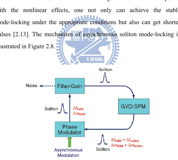
In normal active mode-locked lasers, the optical modulator is driven synchronously with respect to the cavity roundtrip time. In other words, the modulation frequency is equal to the cavity harmonic frequency. However, in the asynchronous soliton mode-locked laser [2.11], the modulation frequency and the cavity harmonic frequency have a small deviation frequency from several kHz to tens kHz [2.12]. For the normal linear optical pulses, they are affected by several kHz frequency shifts, and unstable to achieve stable mode-locking. But for the soliton pulses with the nonlinear effects, one not only can achieve the stable mode-locking under the appropriate conditions but also can get shorter pulses [2.13]. The mechanism of asynchronous soliton mode-locking is illustrated in Figure 2.8.
Fig. 2.8 Laser cavity with the gain, filter, GVD, SPM and the phase modulation driven asynchronously.
The fiber laser is consisted of the gain, the optical bandpass filter, group velocity (GVD), self phase modulation (SPM) and the phase modulator driven asynchronously. Because of asynchronous modulation, the optical pulses reach the optical modulator not always at the peaks of the modulation signal. When the pulse passes through the phase modulator, the central wavelength of the pulse can get a small frequency shift. When the nonlinear effects are not considered, the asynchronous modulation will shift the central frequency of the pulses periodically with accumulation.
Because the gain medium and the filter are both fixed with finite bandwidth, the overdeveloped amount of central frequency shift can make the pulse leave the center of the gain or the filter. Thus the pulses will experience quite large loss such that they cannot exist in the cavity.
On the contrary, the solitons produced by the Kerr nonlinear effects can react against the frequency shift produced by the asynchronous modulation. So the solitons will experience smaller loss and can exist steadily in the cavity, as is shown in Figure 2.9.
Fig.2.9 The noise-cleanup effect in the asynchronous soliton mode-locked laser.
The mechanism explained above is similar to the effects of the sliding-frequency guiding filter [2.14] in the soliton communication systems. The central frequency of the soliton can change with the variation of the center frequency of the filters in the fiber link during propagation, but the center frequency of the linear noise keeps fixed and will be filtered out by the sliding filters. Under the asynchronous soliton mode-locking, one achieves the similar noise-cleanup effects with the fixed center frequency of the filter and the sliding center frequency of the solitons. This provides another advantage for asynchronous mode-locking: a higher SMSR can be obtained, even when there is no explicit intracavity optical device to suppress the supermode noises [2.15].
2.4 The hybrid mode-locking
The hybrid mode-locking approach combines multiple mode-locking techniques within the same laser cavity to improve the laser performance. Hybrid mode-locking usually incorporates the active mode-locking with passive mode-locking. Passively mode-locked lasers can generate very short pulses but typically can not reach very high repetition rates. On the contrary, actively mode-locked laser can generate high repetition rate pulse trains by external modulation but usually can not produce femtosecond pulses.
The most obvious approach is to incorporate an amplitude or phase modulator inside a passively mode-locked fiber laser cavity. Hence the modulator provides periodic timing slots to produce a high rate pulse train while the passive mode-locking mechanism shortens the pulse to a level that can not be expected from active mode-locking alone. This is the kind of setups to be developed in our experiment.
To successfully shorten the pulses in a laser cavity by soliton compression, the following two conditions must be satisfied: [2.16]
(1) The solitons must be successfully re-timed on each round-trip.
(2) There must be discrimination between the soliton state and the actively mode-locked state.
The condition (1) is a practical matter of maintaining synchronism between the modulator and the pulse train and can be automatically achieved by the modulator.
The condition (2) can be quantified by calculating the loss of the soliton and the loss of a fundamental Gaussian pulse, which is the
eigen-solution of the active mode-locking equation (without nonlinearity). If the soliton state is to remain stable, the Gaussian pulse of the active mode-locker must possess a higher loss than that of the soliton. [2.16] The resulting condition is:
24
1
1
+
Re
[
]
3
2
2
2 2 '' 2 2 2 2 2 m m f fM
M
j
L
L
π
τ
β
τ
Ω
Ω
Ω
<
Ω
−
where M is the modulation index per unit length, Ωm is the modulation
frequency, τ is the soliton pulsewidth, Ωf is the filter bandwidth, and β〞
is the GVD over the total cavity length L. On the left side is the net gain that solitons required and on the right side is the net gain that Gaussian pulses required. Following the analysis by Kartner and Kopf [2.17], a sufficiently large amount of negative GVD should suppress the normal mode-locked state enough to allow the formation of a solitary pulse that is considerably shorter than the width predicted by D. K. Kuzenga and A.E.Siegman [2.18]. The main reason is that in this case the soliton parameters of the cavity rather than the modulator characteristics determine the pulsewidth.
R
R
R
e
e
e
f
f
f
e
e
e
r
r
r
e
e
e
n
n
n
c
c
c
e
e
e
[2.1] H. A. Haus, “Mode-locking of lasers,” IEEE J. Select. Topics Quantum Electron, vol. 6, pp. 1173–1185, (2000).
[2.2] M. C. Chan, “Hybrid Mode-locking Er-doped Fiber Laser,” Institute of Electro-Optical engineering in National Chiao-Tung University, master thesis (2002).
[2.3] C. Wu and N. K. Dutta, “High-repetition-rate optical pulse generation using a rational harmonic mode-locked fiber laser,” IEEE J. Quantum Electron., vol. 36, pp. 145–150, (2000).
[2.4] E. Yoshida and M. Nakazawa, “80–200 GHz erbium doped fiber laser using a rational harmonic mode-locking technique,” Electron. Lett., vol. 32, no. 15, pp. 1370–1372, (1996).
[2.5] M. Y. Jeon, H. K. Lee, J. T. Ahn, K. H. Kim, D. S. Lim, and E. H. Lee, “Pulse-amplitude-equalized output from a rational harmonic mode-locked fiber laser,” Opt. Lett. 23, 855–857, (1998).
[2.6] H. J. Lee, K. Kim, H. G. Kim, “Pulse-amplitude equalization of rational harmonic mode-locked fiber laser using a semiconductor optical amplifier loop mirror,” Opt. Commun. 160, 51–56 (1999).
[2.7] Z. Li, C. Lou, K. T. Chan, Y. Li, and Y. Gao, “Theoretical and Experimental Study of Pulse-Amplitude-Equalization in a Rational Harmonic Mode-Locked Fiber Ring Laser,” IEEE J. Quantum Electron. 37, 33–37 (2001).
[2.8] Y. J. Kim, C. G. Lee, Y. Y. Chun, and C.-S. Park, “Pulse-amplitude equalization in a rational harmonic mode-locked semiconductor
fiber ring laser using a dual-drive Mach-Zehnder modulator,” Opt. Express 12, 907 (2004).
[2.9] X. Feng, Y. Lin, S. Yuan, G. Kai, W. Zhong, and X. Dong, IEEE Photon. Technol. Lett. 16, 1813 (2004).
[2.10] S. Yang and X. Bao, “Rational harmonic mode-locking in a phase modulated fiber laser,” IEEE Photon. Technol. Lett., vol. 18, no. 12, pp. 1332–1334, Jun. 15, (2006).
[2.11] C. R. Doerr, H. A. Haus, and E. P. Ippen, “Asynchronous soliton mode locking,” Opt. Lett. 19, 1958-1960 (1994).
[2.12] H. A. Haus, D. J. Jones, E. P. Ippen, and W.S. Wong, “Theory of soliton stability in asynchronous modelocking”, IEEE J. Lightwave Technol., vol. 14, pp. 622-627, (1996).
[2.13] W.-W Hsiang, C.-Y Lin, M.-F Tien, and Y. Lai, “Direct generation of a 10 GHz 816 fs pulse train from an erbium-fiber soliton laser with synchronous phase modulation,” Opt. Lett. 30, 2493-2495 (2005).
[2.14] L. F. Mollenauer, J. P. Gordon, and S. G. Evangelides, ‘‘The sliding frequency guiding filter: an improved form of soliton jitter control,’’ Opt. Lett. 17, 1575 (1992).
[2.15] G. T. Harvey and L. F. Mollenauer, “Harmonically mode-locked fiber ring laser with an internal Fabry-Perot stabilizer for soliton transmission,” Opt. Lett. 18, 107 (1993).
[2.16] D. J. Jones, H. A. Haus, and E. P. Ippen, “Subpicosecond solitons in an actively mode-locked fiber laser,” Opt. Lett. 21, 1818
[2.17] F. X. K¨artner, D. Kopf, and U. Keller, “Solitary-pulse stabilizationand shortening in actively mode-locked laser,”Opt. Soc. Am. B 12, 486 (1995).
[2.18] D. J. KUIZENGA, and A .E. SIEGMAN “FM and AM mode locking of the homogeneous laser,” IEEE J. Quantum Electron. 6, 694 (1970).
Chapter 3
Experimental setup and results
3.1 Experimental setup
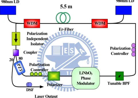
In our experiment, we combine the rational harmonic and asynchronous harmonic modelocking methods to build a new mode-locked fiber laser. The setup is shown in figure 3.1.
Fig. 3.1 The experimental setup
Our setup contains a section of 5.5 meter Erbium-doped fiber pumped by two 980nm laser diodes, which acts as the laser gain medium. The output coupler is put behind the Er-fiber to get the greatest output power. The coupling ratio is 80/20 to couple 20% power inside the laser to the laser output. The chirp of the pulses is compensated with a length of negative group-velocity dispersion (GVD) fiber.
WDM WDM 980nm LD Er-Fiber Tunable BPF LiNbO3 Phase Modulator Polarizer Polarization Controller Polarization Independent Isolator Laser Output DSF Coupler Polarization Controller PZ T 80 20 980nm LD 5.5 m
The isolator in the ring cavity is to ensure the pulses propagate in only one direction. The bandpass filter is used to select the lasing wavelength of the laser. In addition, it can cooperate with self-phase modulation (SPM) effect in the cavity to suppress supermodes and to achieve a high supermode suppression ratio (SMSR). Besides, the wide bandwidth of the bandpass filter can support shorter pulses in the cavity so that the generated pulse width also can be shorter. The devices that have been used in the fiber ring cavity are list in table 3.1.
1. 980nm pump laser : maximum output power: 915mA x 1:500mA x 1 2. EO phase modulator: Vπ=4.7 volt @1GHz
3. Tunable bandpass filter: 13.5nm (3dB bandwidth) ; Central wavelength: 1530~1570nm
4. Polarization independent isolator x 1 5. WDM coupler (980nm/1550nm) x 2 6. Erbium-doped fiber: about 5.5 M 7. Single mode fiber: about 19.33M 8. Coupler:80/20 x 1 ; 95/5 x 1 9. Polarization controller x 2
3.2 Rational harmonic mode-locking results
From section 2.2 we know the rational harmonic mode-locking is induced by the higher order harmonic components of the EO modulation. In general, rational harmonic mode-locking by a phase modulator with a sinusoidal driving signal is difficult to achieve because the modulation harmonic components produced by the phase modulator are too small when the modulation depth is limited. Therefore to generate rational harmonic mode-locking by the phase modulator, one possibility is to produce higher order modulation components by using a nonlinear electronic power amplifier. In this way the rational harmonic mode-locking with a phase modulator can be carried out more easily.
As in figure 3.2, only two very small higher order frequency components are generated by our microwave synthesizer. The fundamental modulation frequency is bigger then other two components about 50dB. In order to generate enough higher order harmonic components we can use a nonlinear power amplifier to enhance the higher order harmonic frequency components. Figure 3.3 is the spectra of the driving signals after the nonlinear power amplifier, which verifies our expectation.
Fig. 3.2 Electronic spectrum from the microwave synthesizer.
Fig. 3.3 Electronic spectrum after the power amplifier.
The fiber length in the experimental setup can be divided into two parts: the single mode fiber length is about 19.33 meters and the Erbium-doped fiber length is about 5.5 meters. The total length is 24.8 meters for this cavity. Therefore the fundamental frequency can be computed to be f0=C/(ngL)=8.3MHz and the net cavity dispersion is around -0.17 ps2. The
bi-directional pumping is utilized in the setup and about 750mW of 980nm pump is used in the laser. A synthesizer is used to generate the RF driving signal which is then amplified to 38dBm.
The electrical driving signal for the phase-modulator is provided by a microwave signal generator (R&S SMR40) and amplified by a power amplifier (Agilent 83017A) with a maximum output power of 1 W. We first operate the modulation frequency at 2.000175GHz and the laser was perfectly mode-locked with the output pulse’s repetition rate around 2GHz. Then we detune the frequency by the amounts of fcav/2, fcav/3,
fcav/4, and the modulation frequency will become 2.000175+8.3MHZ/2,
2.000175+8.3MHZ/3, or 2.000175+8.3MHZ/4. Eventually we can observe the generated pulse repetition rate at 4GHz, 6GHz, and 8GHz. The results in the time and frequency domains are shown in the figures below.
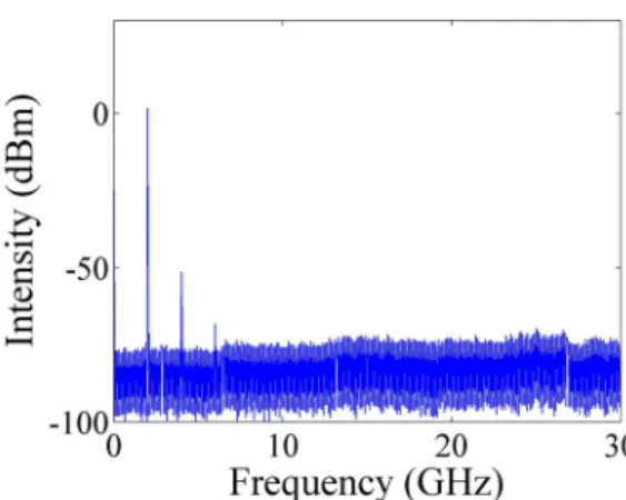
In the frequency domain we show the results of RF spectra in figure 3.4, 3.5, 3.6. The RF spectra are taken with (A) span=30GHz, RBW (resolution bandwidth) =100 kHz (B) span=50MHz, RBW=10 kHz.
(A) Span=30GHz (B) Span=50MHz Fig.3.4 P=2, 4GHz pulse trains in the RF spectrum
(A) Span=30GHz (B) Span=50MHz Fig.3.5 P=3, 6GHz pulse trains in the RF spectrum
(A) Span=30GHz (B) Span=50MHz Fig.3.6 P=4, 8GHz pulse trains in the RF spectrum
As shown in figure 3.4, 3.5, 3.6, we observe certainly the pulse trains
of 4GHz, 6GHz, and 8GHz by rational harmonic mode-locking with p=2, 3, 4. In the RF spectrum with span=30GHz the noise floor is very high. This could be caused by the super-mode noises since the SMSR (super-mode suppression ratio) is smaller than 40dB.
Then in the time domain, we use a fast sampling oscilloscope to
measure the pulse trains. The results are shown in figure 3.7, 3.8, 3.9 with (A) time=100ps/div (B) time=200ps/div.
(A) Time=100ps/div (B) Time=200ps/div. Fig.3.7 P=2, 4GHz pulse trains by the fast sampling oscilloscope.
(A) Time=100ps/div (B) Time=200ps/div. Fig.3.8 P=3, 6GHz pulse trains by the fast sampling oscilloscope.
As show in figure 3.7, 3.8 and 3.9, the pulse trains of 4GHz, 6GHz, 8GHz are clear measured by the sampling scope, indicating the laser is rational harmonic mode-locked at P=2, 3, 4. It can be observed obviously the average pulse amplitude is equal but the amplitude fluctuations and timing jitters that could be caused by the super-mode noises can also be seen.
Next we operate the modulation frequency signal at 4.000375GHz and the laser is rational harmonic mode-locked at p=2, 3. Then we detune the frequency by the amounts of fcav/2, fcav/3, and the modulation frequency
will become 4.000375+8.3MHZ/2, 4.000375+8.3MHZ/3. Same as the previous case, we observe the generated pulse repetition rate at 8GHz and 12GHz. The results in the time and frequency domains are shown in the figures below.
In the frequency domain the RF spectra are shown in figure 3.10, 3.11 with (A) span=30GHz, RBW =100 kHz (B) span=50MHz, RBW=10 kHz.
(A) Span=30GHz (B) Span=50MHz Fig.3.10 P=2, 8GHz pulse trains in the RF spectrum
(A) Span=30GHz (B) Span=50MHz Fig.3.11 P=3, 12GHz pulse trains in the RF spectrum
As show in figure 3.10, 3.11 we can see the side mode suppression ratio become smaller. On the contrary, the super mode noise get higher and the SMSR is just 20dB, which is smaller than before. Hence we know that raising the pulse repetition rate will decrease the side mode suppression ratio at the same time.
Then in the time domain, we use a fast sampling oscilloscope to measure the pulse trains as shown in figure 3.12, 3.13 with (A) time=100ps/div (B) time=200ps/div.
(A) Time=100ps/div (B) Time=200ps/div. Fig.3.13 P=3, 12GHz pulse trains by the fast sampling oscilloscope.
As show in figure 3.12, 3.13 the pulse trains of 8GHz, 12GHz are clearly measured by the sampling scope, where the rational harmonic mode-locking order is P=2, 3. We can observe that the pulse amplitude is equal but it is not too clear, and the pulse trains are losing shape in the high repetition rate because the sampling oscilloscope is not fast enough. In addition the amplitude fluctuations and timing jitters are much higher than at the lower repetition rate.
To summarize, although the pulse amplitude equalization is achieved in our setup by using a phase modulator, the super-mode noises and the amplitude fluctuations seems to be high. In the next section we will not only equalize the pulse amplitude but also suppress the super-mode noises by the asynchronous rational modelocking technique. The pulse width can also be smaller than 1 ps.
3.3 Asynchronous rational harmonic mode-locking results
In the above section, we generated pulse trains of high repetition rate
by rational harmonic mode-locked method. In this section we will generate pulse trains by asynchronous rational harmonic mode-lockeing.
As stated in section 3.1, we first operate the modulation frequency at 2.000175GHZ. Then we detune the frequency by the amounts of fcav/3,
and modulation frequency will become 2.000175+8.3MHZ/3. After that we can observe the generation of pulse repetition rate at 6GHz. At this moment we further detune the modulation frequency with a small amount of kHz. The result in the time domain and frequency domain are shown in the figures below.
In the frequency domain we show the measurement results of RF spectra in figure 3.14 with (A) span=30GHz, RBW (resolution bandwidth) =100 kHz (B) span=50MHz, RBW=10 kHz (C) span=500 kHz.
Then in the time domain, we use a fast sampling oscilloscope to measure the pulse trains and the results are shown in figure 3.15 with (A) time=100ps/div (B) time=200ps/div.
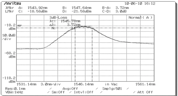
Finally we show the optical spectrum in figure 3.16, the optical bandwidth of output laser is about 3.0nm.
(A) Span=30GHz (B) Span=50MHz
(C) Span=500 KHz
Fig.3.14 P=3, 6GHz pulse trains in the RF spectrum.
(A) Time=100ps/div (B) Time=200ps/div Fig.3.15 P=3, 6GHz pulse trains by the fast sampling oscilloscope.
Fig.3.16 The optical spectrum of the laser output.
As shown in figure 3.14 we observe certainly the pulse trains of 6GHz,
when the modulation frequency is around 2GHz and the laser is asynchronous rational harmonic mode-locked at p=3 with a detuning frequency. In the RF spectrum with span=30GHz the side-mode and super-mode noise suppression are much better than without asynchronous modulation. From figure 3.16 we also can see the full-width at half-maximum (FWHM) bandwidth of the optical spectrum is 3.0nm, which is still not as good as expected. This is because the nonlinear effect is not enough to generate shorter pulse with a low modulation frequency.
Next we operate the modulation frequency at 4.000375GHZ. Then we
detune the frequency by the amounts of fcav/3, and the modulation
frequency will become 4.0003755+8.3MHZ/3. As with the previous case we can observe the generation of pulse repetition rate at 12GHz. Asynchronous modelocking is achieved by further detuning the
shown in the figures below.
In the frequency domain we show the results of RF spectra in figure 3.17, with (A) span=30GHz, RBW (resolution bandwidth) =100 kHz (B) span=50MHz, RBW=10 kHz (C) span=500 kHz.
(A) Span=30GHz (B) Span=50MHz
(C) Span=500 KHz
Fig.3.17 P=3, 12GHz pulse trains in the RF spectrum.
As show in figure 3.17 we observe certainly the pulse trains of 12GHz, when operated with a modulation frequency around 4GHz by rational harmonic mode-locked at p=3 and with some detuning frequency. In the RF spectrum with span=30GHz the side-mode and super-mode noise suppression are again much better than without asynchronous modulation.
From figure 3.17 (B) we could see that the super-mode noise are well suppressed and the SMSR is more than 60dBm. In addition figure 3.18 shows the typical optical spectrum of the laser output and the FWHM bandwidth of the optical spectrum are up to 4.98 nm.
Fig.3.18 The optical spectrum of the laser output.
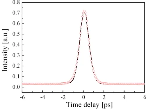
Finally the corresponding second-harmonic generation (SHG) intensity autocorrelation trace is shown in Fig. 3.19 by the solid curve. The empty circle in Fig. 3.19 is the fitting of the SHG intensity autocorrelation trace with the assumption of sech2 pulse shape, indicating that the pulsewidth is 670 fs.
Fig. 3.17 SHG intensity autocorrelation trace (solid curve) and the fitting curve (open circles) of the laser output, assuming sech2 pulse shape.
Finally we operate the modulation frequency at 7.000525GHz. Then we detuned the frequency by the amounts of fcav/3, and the modulation frequency become 7.00525GHz+8.3MHZ/3. We can observe the generated pulse repetition rate at 21GHz. By adding a detuning frequency ~kHz, asynchronous rational harmonic modelocking is achieved. The results in the frequency domain are in the figures below.
In the frequency domain we show the results of RF spectra in figure 3.2 with (A) span=30GHz, RBW=100 kHz (B) span=50MHz, RBW=10 kHz (C) span=500 kHz.
(A) Span=30GHz (B) Span=50MHz
(C) Span=500 KHz
Fig.3.20 P=3, 21GHz pulse trains in the RF spectrum.
As show in figure 3.20 we observe certainly the pulse trains of 21GHz, when operated with a modulation around 7GHz by rational harmonic mode-locked at p=3 and with some detuning frequency. In the RF spectrum with span=30GHz the side-mode and super-mode noise suppression are also suppressed very well.
Similarly, figure 3.21 shows the typical optical spectrum of the laser output and the FWHM bandwidth of the optical spectrum is 3.72 nm.
Fig.3.21 The optical spectrum of the laser output.
Finally the corresponding second-harmonic generation (SHG) intensity autocorrelation trace is shown in Fig. 3.22 by the solid curve. The empty circle in Fig. 3.22 is the fitting of the SHG intensity autocorrelation trace with the assumption of sech2 pulse shape, indicating that the pulsewidth is 900 fs.
Fig. 3.22 SHG intensity autocorrelation trace (solid curve) and the fitting curve (open circles) of laser output, assuming sech2 pulse shape.
Chapter 4
Simulations
4.1 Master equation and variational analyses
We know that an asynchronously mode-locked fiber soliton laser can
be described by the master equation as follows [4.1], [4.2]:
2 2 0 0 + + ) 2 ( )+( + ) 1+ 2 ( , ) ( ) ( , ) ( , | | | | r i r i s g u T t l u T t d jd u T t k jk u u T u dt t E ∂ = − ∂ ∂
∫
∂+
jM
cos[
ω
m(
t RT
+
)
]
(4.1) where u(T,t) is the complex field envelope, g0 is the unsaturated gain, Esis the gain saturation energy, l0 is the linear loss, dr represents the effect of
the optical filtering, di is group velocity dispersion, kr is the effect of
equivalent fast saturable absorption caused by the polarization additive pulse mode-locking (P-APM), ki is the self phase modulation coefficient,
M is the phase modulation strength, ωm is the angular modulation
frequency, T is the number of the cavity round trip, t is the time axis measured in the moving frame propagating at a specific group velocity along with the pulse, and R is the linear timing walk-off per roundtrip due to asynchronous phase modulation [4.3]. In the following analyses, the sinusoidal modulation curve of the phase modulator can be expanded by Taylor’s series as:
2 0 1 0 2 0
cos[
m(
)
]
[
( )
]
[
]
M
ω
t RT
+
≈
m m t t T
−
−
−
m t t
−
(4.2) where (4.3) and (4.4) 1 msin{ [
m 0( )
]}
m
=
M
ω
ω
t T
+
RT
2cos{ [
( )
]}
M
m
=
ω
ω
t T
+
RT
However, the rational harmonic mode locking is based on the frequency detuning of the modulation frequency with respect to the cavity fundamental frequency divided by an integer p. Then the p-order harmonic modulation component must match the cavity harmonic mode to achieve modelocking. Therefore for rational harmonic modelocked fiber lasers we should consider the higher-order modulation harmonic components into the master equation:
2 2 0 0 2 2 )+( + ) ( , )+( + ) 1+ ( , ) ( ) ( , | | | | r i r i s g u T t l u T t d jd u T t k jk u u T u dt t E ∂ = − ∂ ∂
∫
∂ N 1+
M cos[
( +
)]
p m NT
j
N
t
p
ω
=∑
(4.5) Here p is the integer of the rational factor. If we combine asynchronous harmonic mode-locking with rational harmonic mode-locking, the master equation will become:2 2 0 0 ( )+( + ) 2 ( )+( + ) 1+ 2 ( , ) ( ) , , | | | | r i r i s g u T t l u T t d jd u T t k jk u u T u dt t E ∂ = − ∂ ∂
∫
∂ N+
M cos[ ω ( +
+ )]
1 p m NRT T
j
N
t
p
p
=∑
(4.6)The above equations (4.1), (4.5), (4.6) separately described ASML,
RHML, and ARHML. Then they all can be reformulated as a variational
problem by assuming a reasonable pulse solution ansatz [4.4]:
0 + 1+ 0
sec [
( )
]
( ) [ ( )( ( )) ( )]( , )
( )
( )
j T t t T T j Tt t T
u T t
a T
h
T
e
ϖ θ βτ
−−
=
(4.7)pulse timing, β(T) is the chirp, ω(T) is the pulse center frequency, and θ(T) is the phase.
The variational method is applied to solve the above master equation and the evolution equations for all pulse parameters are obtained. The final derived equations for the center frequency, the timing position, the chirp, the amplitude and the pulsewidth are given below:
(4.8) (4.9) (4.10) (4.11) (4.12)
Similarly, the modulation term m1 and m2 must to be changed into: 1
M
sin{N
[
0( )
]}
P N m m NRT
T
m
N
t T
p
p
ω
ω
=
∑
+
+
(4.13) and 2 2 N m 01
M
) cos{N [
]}
2
(
( )
P m NRT T
m
N
t T
p
p
ω
ω
=
∑
+
+
(4.14)In next section we will substitute in all the parameters to obtain numerical
2 1 2 4 (1 ) 3 r d d m dT
β
ω
τ
+ = − − 2 4 2 2 2 2 2 + 2 ( ) 2(2 + )(1+ ) 3 i r i r m a k k d d d dT π τ τ β β β β τ − − = 02
+2
i rdt
d
d
dT
=
ω
βω
2 2 2 4 ( 2 3 ) 9 r r i r d k a d d d d Tτ
β
β
τ
τ
− + + + = − 2 2 2 2 2 0 2[8
6
(
7 9
)]
(
)
9
r i ra k a
d
d
da
g l a
dT
τ
β
β
τ ω
τ
+
−
+ +
=
−
+
4.2 Simulation results of rational harmonic mode-locking
Figures 4.1 show the results of rational harmonic mode-locked (RHML) lasers.
(a) Pulsewidth
(b) Pulse center frequency
(c) Pulse timing position
(d) Pulse energy
Fig. 4.1 Simulation results of RHML evolution equations.
From above figures we can see that the pulsewidth and pulse energy can stably converge to a constant in figure 4.1(a) and (d). Furthermore figure 4.1(b) and (c) also show slight fluctuations of the pulse parameters
4.3 Simulation results of asynchronous rational harmonic
mode-locking
Figures 4.2 show the results of asynchronous rational harmonic mode-locked (ARHML).
(a) Pulse width
(b) Pulse center frequency
(c) Pulse timing position
(d)Pulse energy
We can observe from the above figures that all the pulse parameters exhibit the slow periodic variation at the deviation frequency as shown in figure 4.2(b) and (c). This is similar to the asynchronous harmonic mode-locked fiber laser studied previously [4.3]. In addition, the evolutions of the pulse width and the pulse energy are shown in figure 4.2(a) and (d), which clearly indicates that the oscillation is not purely sinusoidal.
The parameters are estimated based on our experimental observation that output pulses are transform-limited (chirpless) and other measured results. They are g0=4, l0=0.8, dr=0.05, di=0.25, kr=0.1, ki=0.5, Es=0.47,
M=0.3 for all the harmonic modulation components, and p=3. These values should be not far from the actual operating conditions of our laser. The ratio of the cavity roundtrip frequency fc to deviation frequency is
R
R
R
e
e
e
f
f
f
e
e
e
r
r
r
e
e
e
n
n
n
c
c
c
e
e
e
[4.1] H. A. Haus, J. G. Fujimoto, and E. P. Ippen, "Structures for additive pulse mode locking," J. Opt. Soc. Am. B, vol. 8, pp. 2068-2076 ,(1991).
[4.2] H. A. Haus, D. J. Jones, E. P. Ippen and W. S. Wong "Theory of soliton stability in asynchronous modelocking", J. Lightw. Technol., vol. 14, pp. 622 (1996).
[4.3] W.-W. Hsiang, H.-C. C., Y. Lai. "Laser Dynamics of a 10 GHz 0.55 ps Asynchronously Harmonic Modelocked Er-Fiber Soliton Laser", IEEE J. Quantum Electronics 46(3): 292. (2010).
[4.4] D. Anderson, “Variational approach to nonlinear pulse propagation in optical fibers”, Phys. Rev. A, vol. 27, pp. 3135 – 3145, (1983).
Chapter 5
Conclusions
5.1 Summary of achievements
In the thesis we have accomplished the following main achievements. 1. High repetition rate optical pulse generation is typically limited by
the electronic responses in active harmonic mode-locked fiber lasers. We have used the active rational harmonic mode-locking to overcome this problem. By taking advantage of this method it is easy to increase the repetition rate of pulse trains in multiple times.
2. Furthermore, typical rational harmonic mode-locking by amplitude modulation will caused pulse amplitude un-equalization. Additional elements are needed to overcome this problem. In this thesis we have successful achieved the pulse amplitude equalization by rational harmonic mode-locking with phase modulation.
3. Most importantly, we have successfully demonstrated the combination of rational harmonic mode-locking and asynchronous harmonic mode-locking in a hybrid mode-locking fiber laser configuration. We set the modulation signal at a lower frequency of 4GHz or at a higher frequency of 7GHz. With the same rational factor p=3, eventually we have generated pulse trains with the pulsewidth=670fs and SMSR~60dB at 12GHz and pulsewidth=900fs with the same SMSR at 21GHz.
4. Finally, a variational analysis has been developed for studying rational harmonic mode-locked fiber lasers. Synchronous rational harmonic mode-locking will produce a steady state pulse train while asynchronous rational harmonic mode-locking will produce a slowly periodic varying pulse train. All the pulse parameters of the laser output will exhibit slow periodic variation at the deviation frequency.
5.2 Future work
This thesis has successfully demonstrated the high repetition, ultra-short, and low amplitude fluctuation pulse trains. In the future work, we can generate pulse trains of higher repetition rates by operating the modulation frequency at 40GHz and using the rational harmonic mode-locking to multiply the repetition rate three times to 120GHz or even higher. However the required intra-cavity laser power will also increase proportional as the higher repetition rate, if all the operation conditions are kept the same. For the present configuration the 100GHz pulse trains will need about 600mW intra-cavity laser power, which is not small but maybe achievable with the present technologies. By engineering the fiber dispersion and nonlinearity one may be able to somewhat reduce the values. For this reason we will try to increase the intra-cavity laser power as well as to reduce the soliton energy by careful re-design of the laser cavity. This should enable us to demonstrate sub-ps fiber lasers at 100GHz or higher repetition rates.