Introduction to Fortran 90/95
byStephen J. Chapman Grading system:
1. Presence: 30%
2. Midterm: 30%
3. Final: 40%
Office hours: (PH224) 1. Mon. 10:10~12:00 2. Tues. 11:10~12:00 14:40~15:30 3. Fri. 10:10~12:00
Midterm
90 | 99
80 | 89
70 | 79
60 | 69
50 | 59
40 | 49
30 | 39
20 | 29
10 | 19
0 | 9
1 1 1 5 3 15 33 27
Tot: 86 students
Prob. 1(a) 4 + 1 = 5 4 + 2 = 6 2 + 1 = 3 2 + 2 = 4 0 + 1 = 1 0 + 2 = 2 -2 + 1 = -1 -2 + 2 = 0 -4 + 1 = -3 -4 + 2 = -2
Prob. 1(b) n = 2 n = 4 n = 8 n = 10 n = 4
Prob. 1(c)
□□□F□□15□□120.0□test
PROGRAM gave IMPLICIT NONE
CHARACTER (len = 20) :: filename INTEGER :: nvals = 0
INTEGER :: ierror1, ierror2 REAL :: value, x_ave=1.0
WRITE(*,*) 'Please enter input file name:' READ (*,*) filename
OPEN (UNIT = 3, FILE = filename, STATUS = 'OLD', &
ACTION = 'READ', IOSTAT = ierror1) openif: IF(ierror1 ==0) THEN
readloop: DO
READ(3,*, IOSTAT = ierror2) value IF (ierror2 /= 0) EXIT
nvals = nvals + 1 x_ave=x_ave*value
WRITE(*, 1010) nvals, value
Prob. 2
readif: IF (ierror2 > 0) THEN
WRITE(*, 1020) nvals + 1
1020 FORMAT ('Error reading line', I6) ELSE
x_ave=x_ave**(1./nvals)
WRITE(*, 1030) nvals, x_ave
1030 FORMAT ('End of file. There are ', &
I6, ' values in the file.', //'x_ave =' , F7.3) END IF readif
ELSE openif
WRITE(*, 1040) ierror1
1040 FORMAT ('Error opening file: IOSTAT=', I6) END IF openif
CLOSE(3)
END PROGRAM
Test: GAVE.TXT:
1.
2.
4.
output
x_ave = 2.000
Ch. 1 Introduction To Computers And The Fortran Language
Sec. 1.1 The Computer
Fig 1-1Main Memory
Secondary Memory
C P U
(Central processing unit) Input
devices
Output devices
Sec 1.2 Data Representation in a Computer
bit : Each switch represents one binary digit.
ON 1 OFF 0
byte : a group of 8 bits e.g.,
825 MB hard disk. ( 1MB = 106 byte)
Sec 1.2.1 The Binary Number System
The base 10 number system:
1 2 3 10 = 1 x 10² + 2 x 101 + 3 x 100 = 123.
102 101 100
The base 2 number system:
1 0 1 2 = 1 x 22 + 0 x 21 + 1 x 20 = 5
1 1 1 2 = 1 x 22 + 1 x 21 + 1 x 20 = 7 22 21 20
3 bits can represent 8 possible values :
0 ~ 7 (or 000
2~ 111
2)
In general, n bits 2n possible values.
e.g.,
8 bits ( = 1 byte) 28 = 256. (-128 ~ +127)
16 bits ( = 2 byte) 216 = 65,536. (-32,768 ~ +32,767) Sec 1.2.2 Types of Data Stored in Memory
• Character data : (western language, < 256, use 1 byte) A ~ Z (26)
a ~ z (26) 0 ~ 9 (10)
Miscellaneous symbols: ( ) { } ! … Special letters or symbols: à ë …
Coding systems: (see App. A, 8-bit codes)
• ASCII (American Standard Code for Information Interchange)
• EBCDIC (Extended Binary Coded Decimal Interchange Code)
*The unicode coding system uses 2 bytes for each character.
(for any language)
• Integer data: (negative, zero, positive) For an n-bit integer,
Smallest Integer value = - 2n-1 Largest Integer value = 2n-1 - 1 e.g., a 4-byte (= 32-bit) integer,
the smallest = -2,147,483,648 ( = - 232-1) the largest = 2,147,483,647 ( = 232-1-1)
*Overflow condition: An integer > the largest or < the smallest.
• Real data: (or floating-point data) The base 10 system:
299,800,000 = 2.998 x 10⁸ (scientific notation)
mantissa exponent
The base 2 system:
e.g.,
a 4-byte real number = 24-bit mantissa + 8-bit exponent value = mantissa x 2exponent
Precision: The number of significant digits that can be preserved in a number.
e.g., 24-bit mantissa ± 223 (~ seven significant digits) Range: The diff. between the largest and the smallest numbers.
e.g., 8-bit exponent 2-128 ~ 2127 (range ~ 10-38 to 1038)
Sec 1.3 Computer Languages
• Machine language: The actual language that a computer recognizes and executes.
• High-level languages: Basic, C, Fortran, …
*The History of the Fortran Language Fortran = Formula translation
Fortran 66 Fortran 77 Fortran 90 Fortran 95 (1966) (1977) (1991) (1997)
Sec. 2.3 The Structure of a Fortran Statement
A Fortran program = a series of statements
• Executable statements: e.g., additions, subtractions, …
• Non-executable statements: providing information.
Free-source form: Fortran statements may be entered anywhere on a line, up to 132 characters long.
e.g.,
100 output = input1 + input2 ! Sum the inputs or
100 output = input1 & ! Sum the inputs + input2
Sec. 2.4 The Structure of a Fortran Program
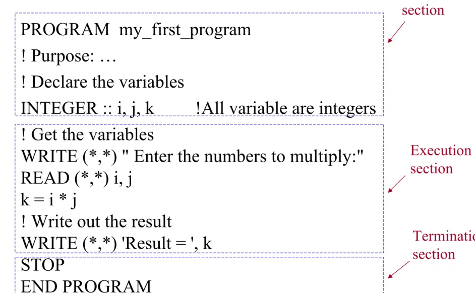
Fig 2-1 (A simple Fortran program) PROGRAM my_first_program ! Purpose: …
! Declare the variables
INTEGER :: i, j, k !All variable are integers ! Get the variables
WRITE (*,*) " Enter the numbers to multiply:"
READ (*,*) i, j k = i * j
! Write out the result
WRITE (*,*) 'Result = ', k STOP
Declaration section
Execution section
Termination section
Sec. 2.4.4 Program Style
Text book :
• Capitalizing Fortran keywords ( e.g., READ, WRITE)
• Using lowercase for variables, parameters
Sec. 2.4.5 Compiling, Linking, and Executing the Fortran Program
Fig 2-2
Fortran
program Object
file
Executable program
(Compile) (Link)
Sec. 2.5 Constants and Variables
Valid variable names: time
distance
z123456789
I_want_to_go_home
(up to 31 chracters, and the 1st character in a name must always be alphabetic)
Invalid variable names: this_is _a_very_long_variable_name 3_days
A$ ($ is an illegal character)
my-help (“-” is an illegal character)
Five intrinsic types of Fortran constants and variables:
1. INTEGER 2. REAL
3. COMPLEX 4. LOGICAL
5. CHARACTER
(numeric) (logical)
(character)
Sec. 2.5.1 Integer Constant and Variables
Integer constants: (no decimal point) e.g.,
0 -999 +17
1,000,000 (X) -100. (X)
Integer variables:
16-bit integers 32-bit integers
(diff. kinds of integers, Ch. 7)
Sec. 2.5.2 Real Constants and Variables
Real constants: (with a decimal point)e.g., 10.
-999.9
1.0E-3 (= 1.0 x 10⁻³ or 0.001) 123.45E20
0.12E+1 1,000,000. (X) 111E3 (X)
Real variables:
32-bit real numbers 64-bit real numbers
(diff. kinds of real numbers, Ch. 7)
Sec. 2.5.3 Character Constants and Variables
Character constants: [enclosed in single (‘) or double (“) quotes)]
e.g.,
‘This is a test!’
“This is a test!”
‘ ‘ (a single blank) ‘{^}’
‘3.141593’ (not a number) This is a test! (X)
‘This is a test!” (X)
A character variable contains a value of the character data type.
Sec. 2.5.4 Logical Constants and Variables
Character constants:
e.g., .TRUE.
.FALSE.
TRUE (X) .FALSE (X)
A logical variable contains a value of the logical data type.
Sec. 2.5.5 Default and Explicit Variable Typing
Default typing: Any variable names beginning with the letters I, J, K, L, M, or N are assumed to be of type INTEGER.
e.g., incr (integer data type)
Explicit typing: The type of a variable is explicitly defined in the declaration section.
e.g.,
PROGRAM example
INTEGER :: day, month, year REAL :: second
LOGICAL :: test1, test2 CHARACTER :: initial
(Executable statements)
*No default names for the character data type!
Sec. 2.5.6 Keeping Constants Consistent in a Program
Using the PARAMETER attribute :
type, PARAMETER :: name=value e.g.,
REAL, PARAMETER :: pi=3.14159
CHARACTER, PARAMETER :: error=‘unknown’
Sec. 2.6 Assignment Statements and Arithmetic Calculations
Assignment statement:variable_name = expression e.g.,
I = I + 1 ( I + 1 I )
Arithmetic operators:
• binary operators:
a + b (a + b, addition) a – b (a – b, subtraction) a * b (a x b, multiplication) a / b (a/b, division)
a ** b (ab, exponentiation)
• unary operators:
+ a - b Rules:
1. No two operators may occur side by side.
e.g.,
a*-b (X) a*(-b) a**-2 (X) a**(-2)
2. Implied multiplication is illegal.
e.g.,
x (y + z) (X) x*(y + z)
3. Parentheses may be used to group terms whenever desired e.g.,
2**((8+2) / 5)
Sec. 2.6.1 Integer Arithmetic
e.g.,
3/4 = 0, 6/4 = 1 7/4 = 1, 9/4 = 2
Sec. 2.6.2 Real Arithmetic (or floating-point arithmetic)
e.g.,
3./4. = 0.75, 6./4. = 1.50
Sec. 2.6.3 Hierarchy (order) of Operators
e.g.,
x = 0.5 * a * t **2 is equal to
x = 0.5 * a * (t **2) ? or
x = (0.5 * a * t ) **2 ? Order:
1. Parentheses, from inward to outward.
2. Exponentials, from right to left.
3. Multiplications and divisions, from left to right.
4. Additions and subtractions, from left to right.
Example 2-1
a = 3. b = 2. c=5. d=4.
e = 10. f = 2. g= 3.
(1) output = a * b + c * d + e / f **g (2) output = a * (b + c) * d + (e / f) **g (3) output = a * (b + c) * (d + e) / f **g Sol.
(1) output = 3. * 2. + 5. * 4. + 10. / 2. ** 3.
= 6. + 20. + 1.25 = 27.25
(2) output = 3. * (2. + 5.) * 4. + (10. / 2.) ** 3.
= 84. + 125.
= 209.
(3) output = 3. * (2. + 5.) * (4. + 10.) / 2. ** 3.
= 3. * 7. * 14. / 8.
= 294. / 8.
= 36.75
Example 2-2
a = 3. b = 2. c=3.
(1) output = a ** (b ** c) (2) output = (a ** b) ** c (3) output = a ** b ** c Sol.
(1) output = 3. ** (2. ** 3.) = 3. ** 8.
= 6561.
(2) output = (3. ** 2.) ** 3.
= 9. ** 3.
= 729.
(3) output = 3. ** 2. ** 3.
= 3. ** 8.
= 6561.
Sec. 2.6.4 Mixed-Mode Arithmetic
In the case of an operation between a real number and an integer, the integer is converted by the computer into a real number.
e.g.,
3. / 2 = 1.5 1 + 1/4 = 1 1. + 1/4 = 1.
1 + 1./4 = 1.25
Automatic type conversion:
e.g.,
nres = 1.25 + 9/4 ave = (5 + 2) / 2 = 1.25 + 2 = 7/2
= 3.25 = 3.
= 3
(a integer variable) (a real variable)
Logarithm
• Base 10:
If 10x = N, then x = ? log N = x
e.g., N = 100 log 100 = log (102) = 2 N = 3 log 3 = 0.47712…
• Base e (=2.71828…): (Natural logarithm)
If ex = N, then x = ? ln N = x
e.g., N = e2 ln (e2) = 2
N = 3 ln 3 = 1.09861…
* If N < 0 ( log N ) or ( ln N ) is undefined !
Sec. 2.6.5 Mixed-Mode Arithmetic and Exponentiation
If result and y are real, and n is an integer, result = y ** n
= y * y * y…*y
(real arithmetic, not mixed-mode) But if result, y and x are real,
result = y ** x = ?
use
y
x= e
x ln y( e ∵
x ln y= e
ln (yx)= y
x)
e.g.,
(4.0) ** 1.5 = 8.
(8.0)**(1./3)=2.
(-2.0) ** 2 = 4. [ (-2.0) * (-2.0) = 4.]∵
(-2.0) ** 2.0 [X, ln (-2.0) is undefined!]∵
Sec. 2.7 Assignment Statements and Logical Calculations
Assignment statements:
logical variable name = logical expression Logical operators:
• relational operators
• combinational operators
Sec. 2.7.1 Relational Operators
a1 op a2
a1, a2: arithmetic expressions, variables, constants, or character strings.
op: the relational logical operators. (see Table 2-3)
Table 2-3
operation meaning = = equal to
/ = not equal to > greater than
> = greater than or equal to < less than
< = less than or equal to e.g.,
operation result 3 < 4 .TRUE.
3 < = 4 .TRUE.
3 = = 4 .FALSE.
‘A’ < ‘B’ .TRUE. (in ASCII, A 65, B 66, p.493) 7+3 < 2+11 .TRUE.
Sec. 2.7.2 Combinational Logic Operators
l1 .op. l2 and .NOT. l1 (.NOT. is a unary operator) l1, l2: logical expressions, variables, or constants.
op: the binary operators. (see Table 2-4) Table 2-4
operation meaning
.AND. logical AND .OR. logical OR
.EQV. logical equivalence
.NEQV. logical non-equivalence
The order of operations:
1. Arithmetic operators.
2. All relational operators, from left to right.
3. All .NOT. operators.
4. All .AND. operators, from left to right.
5. All .OR. operators, from left to right.
6. All .EQV. And .NEQV. operators, from left to right.
Example 2-3
L1 = .TRUE., L2 = .TRUE., L3 = .FALSE.
(a) .NOT. L1 .FALSE.
(b) L1 .OR. L3 .TRUE.
(c) L1 .AND. L3 .FALSE.
(d) L2 .NEQV. L3 .TRUE.
(e) L1 .AND. L2 .OR. L3 .TRUE.
(f) L1 .OR. L2 .AND. L3 .TRUE.
Sec. 2.7.3 The Significance of Logical Variables and Expressions
Most of the major branching and looping structures of Fortran are controlled by logical values.
Sec. 2.8 Assignment Statements and Character Variables
character variables name = character expression Character operators:
1. substring specifications 2. concatenation
Sec. 2.8.1 Substring Specifications
E.g.,
str1 = ‘123456’ str1(2:4) contains the string ‘234’.
Example 2-4
PROGRAM substring
CHARACTER (len=8) :: a,b,c a = ‘ABCDEFGHIJ’
b = ‘12345678’
c = a(5:7)
b(7:8) = a(2:6)
WRITE(*,*) 'a=', a WRITE(*,*) 'b=', b WRITE(*,*) 'c=', c END PROGRAM
a = ? b = ? c = ? (Try it ou
Solu:
a = ‘ABCDEFGH’ ( len = 8)∵ ∵ b(7:8) = a(2:6) = ‘BC’
b = ‘123456BC’
c = a(5:7) = ‘EFG’
= ‘EFG□□□□□‘ ( len = 8)∵
(Cont.)
Sec. 2.8.2 The Concatenation Operator
E.g.,
PROGRAM concate
CHARACTER (len=10) :: a CHARACTER (len=8) :: b,c a = ‘ABCDEFGHIJ’
b = ‘12345678’
c = a(1:3) // b(4:5) // a(6:8) WRITE(*,*)’c=‘,c
END PROGRAM
c = ? (Try it out: c =‘ABC45FGH’)
Sec. 2.8.3 Relational Operators with Character Data
E.g.,
‘123’ = = ‘123’ (true) ‘123’ = = ‘1234’ (false)
‘A’ < ‘B’ (true, ASCII, A 65, B 66)∵ ‘a’ < ‘A’ (false, a 97)∵
‘AAAAAB’ > ‘AAAAAA’ (true) ‘AB’ > ‘AAAA’ (true)
‘AAAAA’ > ‘AAAA’ (true)
Sec. 2.9 Intrinsic Functions
• Intrinsic functions are the most common functions built directly into the Fortran language. ( see Table 2-6 and App. B)
• External functions are supplied by the user. (see Ch. 6) e.g.,
y = sin(3.141593) INT(2.9995) = 2
(truncates the real number) y = sin(x)
y = sin(pi*x) NINT(2.9995) = 3
(rounds the real number) y = sin(SQRT(x))
Generic functions: (can use more than one type of input data) e.g.,
If x is a real number, ABS(x) is real.
If x is an integer,
ABS(x) is integer.
Specific functions: (can use only one specific type of input data) e.g.,
IABS(i)
(integer only)
*See Appendix B for a complete list of all intrinsic functions.
Sec. 2.10 List-directed (or free-format) Input and Output Statements
• The list-directed input statement:
READ (*,*) input_list I/O unit format
• The list-directed output statement:
WRITE (*,*) output_list I/O unit format
e.g.,
PROGRAM input_example INTEGER :: i, j
REAL :: a
CHARACTER (len=12) :: chars READ(*,*) i, j, a, chars
WRITE(*,*) i, j, a, chars END PROGRAM
Input: 1, 2, 3., ‘This one.’ (or 1 2 3. ‘This one.’) Output: 1 2 3.00000 This one.
(Try it out!)
Sec. 2.11 Initialization of Variables
E.g.,
PROGRAM init INTEGER :: i WRITE(*,*) I
END PROGRAM
Output: i = ??? (uninitialized variable)
Run-time error! (depends on machines)
(Try it out!)
Three ways to initialize variables:
1. Assignment statements:
e.g.,
PROGRAM init_1 INTEGER :: i
i = 1
WRITE(*,*) i
END PROGRAM 2. READ statements:
e.g.,
PROGRAM init_2 INTEGER :: i
READ(*,*) i WRITE(*,*) i
END PROGRAM
3. Type declaration Statements:
type :: var1 = value1, [var2 = value2, …]
e.g.,
REAL :: time = 0.0, distance = 5128.
INTEGER :: loop = 10
LOGICAL :: done = .FALSE.
CARACTER (len=12) :: string = ‘characters’
or
PROGRAM init_3 INTEGER :: i = 1 WRITE(*,*) i
END PROGRAM
Sec. 2.12 The IMPLICIT NONE Statement
When the IMPLICIT NONE statement is included in a program, any variable that does not appear in an explicit type declaration statement is considered an error.
e.g.,
PROGRAM test_1 REAL :: time
time = 10.0
WRITE(*,*) ‘Time=‘, tmie END PROGRAM
Output:
Run-time error! (depends on machines)
+ IMPLICIT NONE,
PROGRAM test_1 IMPLICIT NONE REAL :: time
time = 10.0
WRITE(*,*) ‘Time=‘, tmie END PROGRAM
Output:
Compile-time error! (depends on machines)
Sec. 2.13 Program Examples
Example 2-5 (Temperature conversion) T (0F) = (9/5) T(0C) + 32
Fig. 2-6
PROGRAM temp IMPLICIT NONE
REAL :: temp_c, temp_f
WRITE(*,*) ’Enter T in degrees C:’
READ(*,*) temp_c
temp_f = (9./5.) * temp_c + 32.
WRITE(*,*) temp_c,’ degrees C =‘, temp_f, &
‘degrees F’
END PROGRAM (Try it out!)
Example (extra)
Write a program for converting a 4 bits integer into a base 10 number, e.g.,
1 0 1 1 = 1 x 23 + 0 x 22 + 1 x 21 + 1 x 20 = 11
Ch. 3 Control Structures and Program Design
Ch. 2: Sequential programs (simple and fixed order)
Here: Complex programs (using two control statements)
(1) branches (2) loops
Sec. 3.1 Introduction to Top-down Design Techniques
Start
State the problem
Design the algorithm
Convert algorithm into Fortran statements
Test the program
Finished !
Fig. 3-1 (a formal program design process)
Sec. 3.2 Pseudocode and Flowcharts
(1) Pseudocode : a mixture of Fortran and English (2) Flowcharts : graphical symbolsl
e.g.,
(1) The pseudocode for Example 2-5:
Prompt user to enter temp. in degree Farenheit Read temp. in degree Farenheit
temp_k in Kelvins (5./9.)*(temp_f-32.)+273.15 Write temp. in Kelvins
(2) The flowcharts for Example 2-5:
Start Tell user to enter temp_f
Get temp_f
Calculate
temp_k Write temp_k Stop
(an oval for start or stop)
(a parallelogram for I/O)
Sec. 3.3 Control Constructs: Branches
• IF Statement
• SELECT CASE
Branches are Fortran statements that permit us to select and execute specific sections of code (called blocks) while skipping other sections of code.
Sec. 3.3.1 The Block IF Construct
This construct specifies that a block of code will be executed if and only if a certain logical expression is true.
IF (logical_expr) THEN Statement 1
Statement 2 .
. . END IF
a block
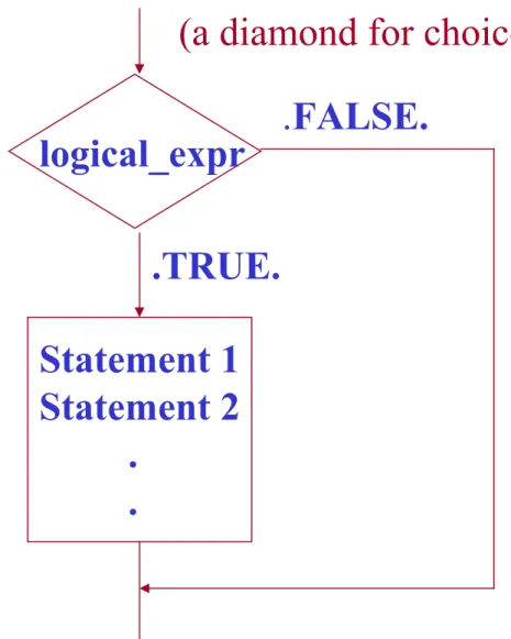
Fig . 3-5 (Flowchart for a simple block IF construct)
logical_expr
Statement 1 Statement 2 .
.
.TRUE.
.FALSE.
(a diamond for choice)
Example:
ax2 + bx + c = 0,
x = -b ± ( b2 – 4ac )1/2 2a
If b2 – 4ac = 0 b2 – 4ac > 0
b2 – 4ac < 0
two distinct real roots
two complex roots a single repeated root
Fig . 3-6 (Flowchart)
.TRUE.
.FALSE.
Problem: Tell the user if the eq. has complex roots.
b2 – 4ac < 0
WRITE ‘two complex roots’
Fortran:
IF ( (b**2 – 4.*a*c) < 0. ) THEN
WRITE(*,*) ‘Two complex roots!’
END IF
Sec. 3.3.2 The ELSE and ELSE IF Clauses
For many different options to consider,
IF + ELSE IF (one or more) + an ELSE
IF (logical_expr_1) THEN Statement 1
Statement 2 .
.
ELSE IF (logical_expr_2) THEN Statement 1
Statement 2 .
. ELSE
Statement 1 Statement 2 .
. END IF
Block 1
Block 2
Block 3
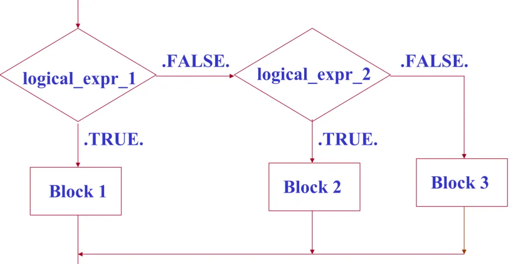
Fig . 3-7 (flowchart)
.TRUE.
.FALSE.
logical_expr_1
Block 1
logical_expr_2
Block 2
.TRUE.
.FALSE.
Block 3
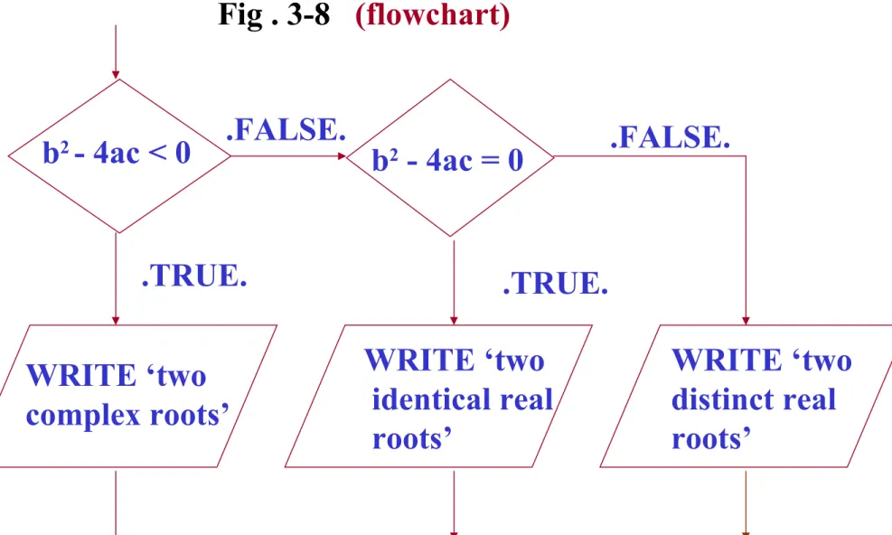
Fig . 3-8 (flowchart)
.TRUE.
.FALSE.
b2 - 4ac < 0
WRITE ‘two complex roots’
.TRUE.
.FALSE.
Example: Tell the user whether the eq. has two complex roots, two identical real roots, or two distinct real roots.
b2 - 4ac = 0
WRITE ‘two identical real roots’
WRITE ‘two distinct real roots’
Fortran:
IF ( (b**2 – 4.*a*c) < 0. ) THEN
WRITE(*,*) ‘two complex roots’
ELSE IF ( (b**2 – 4.*a*c) == 0. ) THEN WRITE(*,*) ‘two identical real roots’
ELSE
WRITE(*,*) ‘two distinct real roots’
END IF
Write a complete Fortran program for a quadratic equation ax2 + bx + c = 0.
Input: a, b, c (e.g., 1., 5., 6.
or 1., 4., 4.
or 1., 2., 5.)
Output: ‘distinct real’
or ‘identical real’
or ‘complex roots’
(Try it out!)
PROGRAM abc IMPLICIT NONE REAL :: a, b, c
WRITE(*,*)'Enter the coeffs. a, b, and c:‘
READ(*,*) a, b, c
IF ( (b**2-4.*a*c) < 0. ) THEN WRITE(*,*) 'two complex root‘
ELSE IF ( (b**2-4.*a*c) == 0. ) THEN WRITE(*,*) 'two identical real roots‘
ELSE
WRITE(*,*) 'two distinct real roots‘
END IF
END PROGRAM
Sec. 3.3.3 Examples Using Block IF Constructs
Example 3-1 The Quadratic Equation: (ax2 + bx + c =0) Write a program to solve for the roots of a quadratic equation, regardless of type.
Input: a, b, c
Output: roots
real
repeated real complex
PROGRAM root IMPLICIT NONE
REAL :: a, b, c, d, re, im, x1, x2
WRITE(*,*)'Enter the coeffs. a, b, and c:‘
READ(*,*) a, b, c d = b**2 – 4.*a*c IF ( d < 0. ) THEN
WRITE(*,*) 'two complex root:‘
re = (-b)/(2.*a)
im = sqrt(abs(d))/(2.*a)
WRITE(*,*) ’x1=‘, re, ‘+ i’, im WRITE(*,*) ’x2=‘, re, ‘- i’, im ELSE IF ( d == 0. ) THEN
WRITE(*,*) 'two identical real roots:‘
x1 = (-b) / (2.*a)
WRITE(*,*) ’x1=x2=‘, x1
ELSE
WRITE(*,*) 'two distinct real roots:‘
x1 = (-b + sqrt(d)) / (2.*a) x2 = (-b – sqrt(d)) / (2.*a) WRITE(*,*) ’x1=‘, x1
WRITE(*,*) ‘x2=‘, x2 END IF
END PROGRAM
Test: (Try it out!)
x2 + 5x + 6 = 0, x1,2 = -2, -3 x2 + 4x + 4 = 0, x1,2 = -2
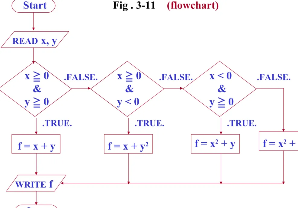
Example 3-2 Evaluation a Function of Two Variables:
f(x,y) =
x + y, x 0 ≧ and y 0≧ x + y2, x 0 ≧ and y < 0 x2 + y, x < 0 and y 0≧ x2 + y2, x < 0 and y < 0
Input: x, y
Output: f
Fig . 3-11 (flowchart)
.TRUE.
.FALSE.
x ≧ 0 &
y 0≧
f = x + y
x 0 ≧ &
y < 0
f = x2 + y
.TRUE.
.FALSE.
f = x2 + y2 f = x + y2
x < 0 &
y 0≧
.TRUE.
.FALSE.
WRITE f Start
READ x, y
PROGRAM funxy IMPLICIT NONE REAL :: x, y, f
WRITE(*,*)'Enter x and y:‘
READ(*,*) x, y
IF ((x >= 0.) .AND. (y >= 0. )) THEN f = x + y
ELSE IF ((x >= 0.) .AND. (y < 0. )) THEN f = x + y**2
ELSE IF ((x < 0.) .AND. (y >= 0. )) THEN f = x**2 + y
ELSE
f = x**2 + y**2 END IF
WRITE(*,*) ‘f = ‘, f END PROGRAM
Test: (Try it out!) x y f 2. 3. 5.
2. -3. 11.
-2. 3. 7.
-2. -3. 13.
[name:] IF (logical_expr_1) THEN Statement 1
Statement 2 .
.
ELSE IF (logical_expr_2) THEN [name]
Statement 1 Statement 2 .
.
ELSE [name]
Statement 1 Statement 2 .
.
END IF [name]
Block 1
Block 2
Block 3
Sec. 3.3.4 Named Block IF Constructs
optional
optional
Sec. 3.3.5 Notes Concerning the Use of Logical IF Constructs
Nested IF Constructs:
outer: IF ( x > 0. ) THEN .
.
inner: IF ( y < 0. ) THEN .
. END IF inner .
.
Example 3-3 Assigning Letter Grades:
95 < GRADE A 86 < GRADE < 95 B 76 < GRADE < 86 C 66 < GRADE < 76 D 0 < GRADE < 66 F
Input: grade
Output: ‘The grade is A.’
or ‘The grade is B.’
or ‘The grade is C.’
or ‘The grade is D.’
or ‘The grade is F.’
Method (a): IF + ELSE IF IF (grade > 95.) THEN
WRITE(*,*) ‘The grade is A.’
ELSE IF (grade > 86.) THEN
WRITE(*,*) ‘The grade is B.’
ELSE IF (grade > 76.) THEN
WRITE(*,*) ‘The grade is C.’
ELSE IF (grade > 66.) THEN
WRITE(*,*) ‘The grade is D.’
ELSE
WRITE(*,*) ‘The grade is F.’
END IF
Method (b): nested IF
if1: IF (grade > 95.) THEN
WRITE(*,*) ‘The grade is A.’
ELSE
if2: IF (grade > 86.) THEN
WRITE(*,*) ‘The grade is B.’
ELSE
if3: IF (grade > 76.) THEN
WRITE(*,*) ‘The grade is C.’
ELSE
if4: IF (grade > 66.) THEN
WRITE(*,*) ‘The grade is D.’
ELSE
WRITE(*,*) ‘The grade is F.’
END IF if4 END IF if3 END IF if2 END IF if1
Sec. 3.3.6 The Logical IF Statement
IF (logical_expr) Statement
e.g.,
IF ( (x >= 0.) .AND. (y >= 0.) ) f = x + y
[name:] SELECT CASE (case_expr) CASE (case_selector_1) [name]
Statement 1 Statement 2 . . .
CASE (case_selector_2) [name]
Statement 1 Statement 2 . . .
CASE DEFAULT [name]
Statement 1 Statement 2 . . .
END SELECT [name]
Block 1
Block 2
Block 3
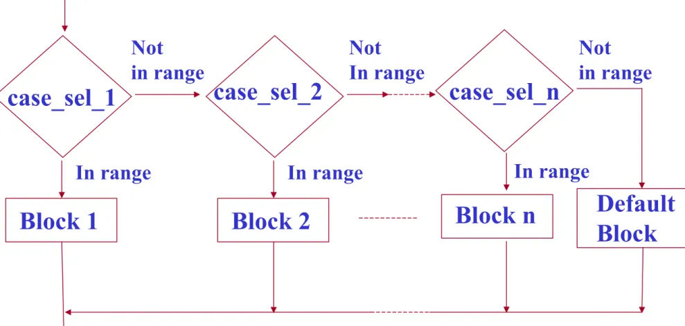
Sec. 3.3.7 The CASE Construct
optional
optional
optional
case_expr: an integer, character, or logical expression.
The case_selector can take one of four forms:
1. case_value Execute block if case_value == case_expr 2. low_value: Execute block if low_value <= case_expr 3. : high_value: Execute block if case_expr <= high_value 4. low value: high_value
Execute block if low_value <= case_expr <= high_value
Fig . 3-13 (flowchart for a CASE construct)
In range Not
in range
case_sel_1
Block 1
case_sel_2
Block n
In range Not
In range
Default Block Block 2
case_sel_n
In range Not
in range
e.g., (modified)
REAL :: temp_c . . .
temp: SELECT CASE (temp_c) CASE (: -1.0)
WRITE (*,*) ‘ It’s below freezing today!’
CASE (0.0)
WRITE (*,*) ‘ It’s exactly at the freezing point!’
CASE (1.0:20.0)
WRITE (*,*) ‘ It’s cool today!’
CASE (21.0:33.0)
WRITE (*,*) ‘ It’s warm today!’
CASE (34.0:)
WRITE (*,*) ‘ It’s hot today!’
PROGRAM selectc IMPLICIT NONE INTEGER :: temp_c
WRITE(*,*) “Enter today’s temp. in degree C:”
READ(*,*) temp_c
temp: SELECT CASE (temp_c) CASE (: -1)
WRITE (*,*) “It’s below freezing today!”
CASE (0)
WRITE (*,*) “It’s exactly at the freezing point!”
CASE (1:20)
WRITE (*,*) “It’s cool today!”
CASE (21:33)
WRITE (*,*) “It’s warm today!”
CASE (34:)
WRITE (*,*) “It’s hot today!”
END SELECT temp END PROGRAM
Problem: Determine whether an integer between 1 and 10 is even or odd. (Try it out!)
PROGRAM selectv INTEGER :: value
WRITE(*,*) 'Enter an inter between 1-10:' READ(*,*) value
SELECT CASE (value) CASE (1,3,5,7,9)
WRITE(*,*) 'The value is odd.' CASE (2,4,6,8,10)
WRITE(*,*) 'The value is even.' CASE (11:)
WRITE(*,*) 'The value is too high' CASE DEFAULT
WRITE(*,*) 'The value is negative or zero.' END SELECT
Sec. 3.4 Control Constructs: Loops
• while loops
• iterative (or counting) loops
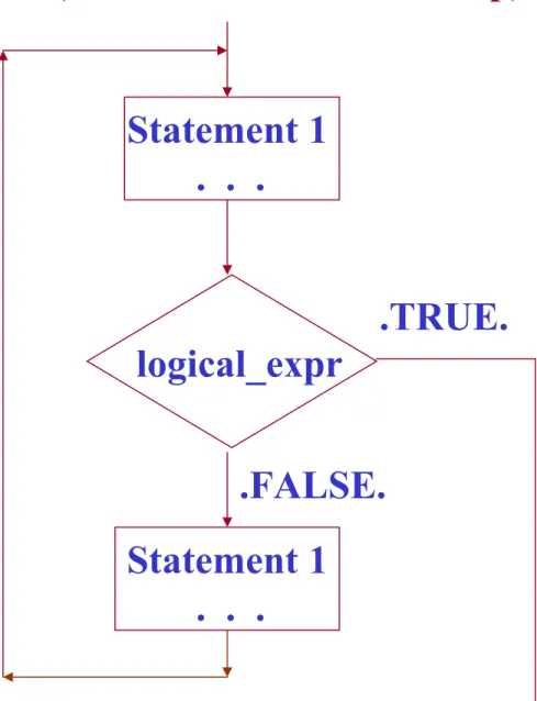
Sec. 3.4.1 The While Loop
DO . . .
IF (logical_expr) EXIT . . .
END DO
a code block
Fig . 3-14 (Flowchart for a while loop)
.TRUE.
.FALSE.
logical_expr Statement 1 . . .
Statement 1 . . .
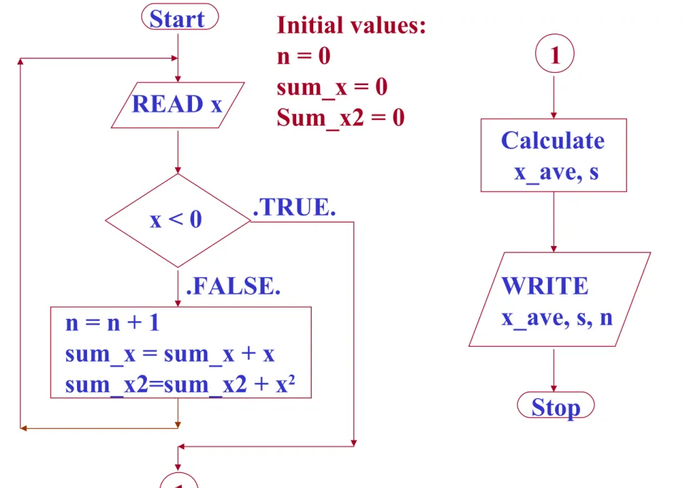
Example 3-4 Statiscal Analysis:
Average:
x_ave =
Σ
xii=1 N
N Standard deviation:
S =
N
Σ
xi2 – (i=1 i=1
N N
Σ
xi )2 N (N-1)1/2
Input: x (i.e., xi , i = 1, 2, …, N) 0 ≧ Output: x_ave and S
Fig . 3-15 (Flowchart for Example 3-4)
.TRUE.
.FALSE.
x < 0 READ x
n = n + 1
sum_x = sum_x + x sum_x2=sum_x2 + x2
Start
1
Calculate x_ave, s
Stop WRITE x_ave, s, n Initial values:
n = 0
sum_x = 0 Sum_x2 = 0
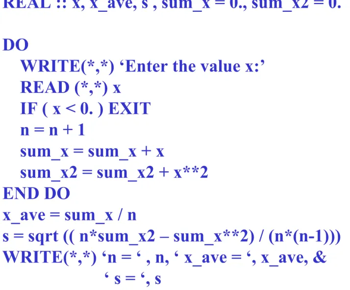
Fig . 3-16 PROGRAM stats_1 IMPLICIT NONE INTEGER :: n = 0
REAL :: x, x_ave, s , sum_x = 0., sum_x2 = 0.
DO
WRITE(*,*) ‘Enter the value x:’
READ (*,*) x
IF ( x < 0. ) EXIT n = n + 1
sum_x = sum_x + x
sum_x2 = sum_x2 + x**2 END DO
x_ave = sum_x / n
s = sqrt (( n*sum_x2 – sum_x**2) / (n*(n-1))) WRITE(*,*) ‘n = ‘ , n, ‘ x_ave = ‘, x_ave, &
‘ s = ‘, s END PROGRAM
Test:
Input: 3.
4.
5.
-1.
Output: n = 3 x_ave = 4.00000 s = 1.00000
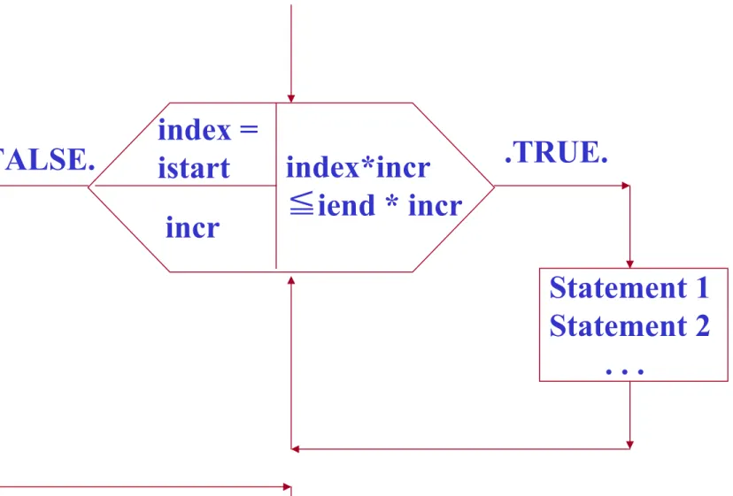
Sec. 3.4.2 The Iterative Counting Loop
DO index = istart, iend, incr Statement 1
. . .
Statement n END DO
e.g.,
(1) Do i = 1, 10 Statement 1 . . .
Statement n END DO
( incr = 1 by default)
(2) Do i = 1, 10, 2 Statement 1 . . .
Statement n END DO
( i = 1, 3, 5, 7, 9 )
Fig. 3-18 (Flowchart for a Do loop construct)
index*incr
≦iend * incr index =
istart incr
Statement 1 Statement 2 . . .
.TRUE.
.FALSE.
Example 3-5 The Factorial Function:
N ! = N × (N-1) × (N-2) … × 3 × 2 × 1, N > 0.
0 ! = 1 e.g.,
4 ! = 4 × 3 × 2 × 1 = 24 5 ! = 5 × 4 × 3 × 2 × 1 = 120
Fortran Code: n_factorial = 1 DO i = 1, n
n_factorial = n_factorial * i END DO
Problem: Write a complete Fortran program for the factorial function.
Input: n ( n > = 0 )
N ! = N × (N-1) × (N-2) … × 3 × 2 × 1, N > 0.
0 ! = 1
Output: n!
PROGRAM factorial IMPLICIT NONE
INTEGER :: i, n, n_fact
WRITE(*,*) ’Enter an integer n ( > = 0 ):’
READ(*,*) n n_fact = 1
IF ( n > 0 ) THEN DO i = 1, n
n_fact = n_fact * i END DO
END IF
WRITE(*,*) n, ‘! = ‘, n_fact END PROGRAM
Fig . 3-20
.TRUE. .FALSE.
n < 2 READ n
sum_x =
sum_x + x sum_x2 =
sum_x2+x2 Start
1
1
Calculate x_ave, s WRITE x_ave, s, n
Initial values:
sum_x = 0 sum_x2 = 0
Example 3-7 Statistical Analysis: (modified)
WRITE
‘At least 2 values!’
i=1
i=i+1 i n≦ ?
READ x
.FALSE. .TRUE.
Fig . 3-21
PROGRAM stats_3 IMPLICIT NONE INTEGER :: i, n
REAL :: x, x_ave, s , sum_x = 0., sum_x2 = 0.
WRITE(*,*) ‘Enter the number of points n:’
READ(*,*) n
IF ( n < 2 ) THEN
WRITE(*,*) ‘ At least 2 values!’
ELSE
DO i = 1, n
WRITE(*,*) ‘Enter the value x:’
READ (*,*) x
sum_x = sum_x + x
sum_x2 = sum_x2 + x**2 END DO
x_ave = sum_x / n
s = sqrt (( n*sum_x2 – sum_x**2) / (n*(n-1))) WRITE(*,*) ‘n = ‘ , n, ‘ x_ave = ‘, x_ave, &
‘ s = ‘, s END IF
END PROGRAM
Test:
Input: 3 3.
4.
5.
Output: n = 3 x_ave = 4.00000 s = 1.00000
Sec. 3.4.3 The CYCLE and EXIT Statements
E.g.,
PROGRAM test_cycle INTEGER :: i
DO i = 1, 5
IF ( i == 3 ) CYCLE WRITE(*,*) i
END DO
WRITE(*,*) ‘End of loop!’
END PROGRAM
Output: 1
2 4 5 End of loop!
PROGRAM test_exit INTEGER :: I
DO i = 1, 5
IF ( i == 3 ) EXIT WRITE(*,*) i
END DO
WRITE(*,*) ‘End of loop!’
END PROGRAM
Output: 1
2 End of loop!
[name:] DO . . .
IF (logical_expr) CYCLE [name]
. . .
IF (logical_expr) EXIT [name]
. . .
END DO [name]
Sec. 3.4.4 Named Loops
While loop:
optional
[name:] DO index = istart, iend, incr . . .
IF (logical_expr) CYCLE [name]
. . .
END DO [name]
Counting loop:
optional
Sec. 3.4.5 Nesting Loops and Block IF Construct
e.g.,
PROGRAM nested_loops INTEGER :: i, j, product DO i = 1, 3
DO j = 1, 3
product = i * j
WRITE(*,*) i, ‘*’, j, ‘=‘, product END DO
END DO
END PROGRAM
Output:
1 * 1 = 1 1 * 2 = 2 1 * 3 = 3 2 * 1 = 2 2 * 2 = 4 2 * 3 = 6 3 * 1 = 3 3 * 2 = 6 3 * 3 = 9
PROGRAM test_cycle_1 INTEGER :: i, j, product DO i = 1, 3
DO j = 1, 3
IF ( j == 2 ) CYCLE product = i * j
WRITE(*,*) i, ‘*’, j, ‘=‘, product END DO
END DO
END PROGRAM Output: 1 * 1 = 1
1 * 3 = 3 2 * 1 = 2 2 * 3 = 6 3 * 1 = 3 3 * 3 = 9
PROGRAM test_cycle_2 INTEGER :: i, j, product outer: DO i = 1, 3
inner: DO j = 1, 3
IF ( j == 2 ) CYCLE outer product = i * j
WRITE(*,*) i, ‘*’, j, ‘=‘, product END DO inner
END DO outer END PROGRAM
Output:
1 * 1 = 1 2 * 1 = 2 3 * 1 = 3
Nesting loops within IF constructs and vice versa:
e.g.,
outer: IF ( a < b ) THEN . . .
inner: DO i = 1, 3 . . .
ELSE
. . .
END DO inner END IF outer
illegal!
outer: IF ( a < b ) THEN . . .
inner: DO i = 1, 3 . . .
END DO inner . . .
ELSE
. . .
END IF outer legal:
Ch. 4 Basic I/O Concepts
Sec. 4.1 FORMATS and FORMETED WRITE STATEMENTS
READ (*,*) Not always convenient!
WRITE (*,*) Not always pretty!
e.g,. PROGRAM free_format INTEGER :: i = 21
REAL :: result = 3.141593 WRITE(*,100) i, result
100 FORMAT (‘□The□result□for□iteration□’, &
I3, ‘□is□’, F7.3) END PROGRAM
Output: □The□result□for□iteration□□21□is□□□3.142
∵ I3 ∵ F7.3
The following three WRITE statements are equivalent:
• WRITE (*, 100) i, result 100 FORMAT (I6, F10.2)
• CHARACTER ( len=20 ) :: string string = ‘(I6, F10.2)’
WRITE(*,string) i, result
• WRITE(*, ‘(I6,F10.2)’) i, result
Output: □□□□21□□□□□□3.14
I6 F10.2
PROGRAM format INTEGER :: i = 21
REAL :: result = 3.141593
CHARACTER ( len=20 ) :: string WRITE (*, 100) i, result
100 FORMAT (I6, F10.2) string = '(I6, F10.2)'
WRITE(*,string) i, result
WRITE(*, '(I6,F10.2)') i, result END PROGRAM
Output: □□□□21□□□□□□3.14
Sec. 4.2 Output Devices
Line printers, laser printers, and terminals.
Sec. 4.3 Format Descriptors
Table 4-2 (Symbols used with format descriptors) Symbol meaning
c column number
d # of digits to the right of the decimal point m min. # of digit
r repeat count w field width
Sec. 4.3.1 Integer Output – The I Descriptor
rIw or rIw.m e.g.,
INTEGER :: index = -12, junk = 4, number = -12345 WRITE(*,200) index, index+12, junk, number
WRITE(*,210) index, index+12, junk, number WRITE(*,220) index, index+12, junk, number 200 FORMAT ( 2I5, I6, I10)
210 FORMAT (2I5.0, I6, I10.8) 220 FORMAT (2I5.3, I6, I5)
Output:
□□-12□□□□0□□□□□4□□□□-12345 □□-12□□□□□□□□□□4□-00012345 □-012□□000□□□□4*****
(Not in scale!)
I5 I5 I6 I10
PROGRAM iformat IMPLICIT NONE
INTEGER :: index = -12, junk = 4, number = -12345 WRITE(*,200) index, index+12, junk, number
WRITE(*,210) index, index+12, junk, number WRITE(*,220) index, index+12, junk, number 200 FORMAT ( 2I5, I6, I10)
210 FORMAT (2I5.0, I6, I10.8) 220FORMAT (2I5.3, I6, I5)
END PROGRAM
Output: -12 0 4 -12345
-12 4 -00012345 (Not in scale!)
Sec. 4.3.2 Real Output – The F Descriptor
rFw.d e.g.,
REAL :: a = -12.3, b = .123, c = 123.456 WRITE(*,200) a, b, c
WRITE(*,210) a, b, c
200 FORMAT (2F6.3, F8.3) 210 FORMAT (3F10.2)
Output: ******□0.123□123.456
□□□□-12.30□□□□□□0.12□□□□123.46
(Not in scale!) F6.3 F6.3 F8.3
F10.2 F10.2 F10.2
PROGRAM rformat IMPLICIT NONE
REAL :: a = -12.3, b = .123, c = 123.456 WRITE(*,200) a, b, c
WRITE(*,210) a, b, c
200 FORMAT (2F6.3, F8.3) 210 FORMAT (3F10.2)
END PROGRAM
Output: ****** 0.123 123.456
-12.30 0.12 123.46
Sec. 4.3.3 Real Output – The E Descriptor
(Expomential notation) Scientific notation: 6.02 × 10²³
Exponential notation: 0.602 × 1024 (E Descriptor)
0.602 E+24 rFw.d ( w d + ≧ 7 )
e.g., REAL :: a = 1.2346E6, b = 0.001, c = -77.7E10, d = -77.7E10 WRITE (*,200) a, b, c, d
200 FORMAT (2E14.4, E13.6, E11.6)
□□□□0.1235E+07□□□□0.1000E-02-0.777000E+12***********
E14.4 E14.4 E13.6 E11.6
Output:
( ‘E+**’ , ‘0.’, and ‘-’)∵
( 11 < 6 + 7)∵
PROGRAM routput IMPLICIT NONE
REAL :: a = 1.2346E6, b = 0.001, c = -77.7E10, d = -77.7E10 WRITE (*, 200) a, b, c, d
200 FORMAT (2E14.4, E13.6, E11.6) END PROGRAM
Sec. 4.3.4 True Scientific Notation – The ES Descriptor
rESw.d ( w d + ≧ 7 ) e.g.,
REAL :: a = 1.2346E6, b = 0.001, c = -77.7E10 WRITE (*,200) a, b, c
200 FORMAT (2ES14.4, ES12.6)
□□□□1.2346E+06□□□□1.0000E-03************
ES14.4 ES14.4 ES12.6
Output:
PROGRAM esformat IMPLICIT NONE
REAL :: a = 1.2346E6, b = 0.001, c = -77.7E10 WRITE (*, 200) a, b, c
200 FORMAT (2ES14.4, ES12.6) END PROGRAM
Sec. 4.3.5 Logical Output – The L Descriptor
rLw e.g.,
LOGICAL :: output = .TRUE., debug = .FALSE.
WRITE (*, 200) output, debug 200 FORMAT (2L5)
□□□□T□□□□F
L5 L5
Output:
PROGRAM loutput IMPLICIT NONE
LOGICAL :: output = .TRUE., debug = .FALSE.
WRITE (*, 200) output, debug 200 FORMAT (2L5)
END PROGRAM
Sec. 4.3.6 Character Output – The A Descriptor
rAw or rA e.g.,
CHARACTER (len = 17) :: string = ‘This□is□a□string.’
WRITE (*, 10) string WRITE (*, 11) string WRITE (*, 12) string 10 FORMAT (A) 11 FORMAT (A20) 12 FORMAT (A6) Output:
(i.e., the width is the same as the # of characters being displayed.)
17 characters
This□is□a□string.
□□□This□is□a□string.
This□i
PROGRAM aoutput IMPLICIT NONE
CHARACTER (len = 17) :: string = 'This is a string.‘
WRITE (*, 10) string WRITE (*, 11) string WRITE (*, 12) string 10 FORMAT (A)
11 FORMAT (A20) 12 FORMAT (A6) END PROGRAM
Sec. 4.3.7 Horizontal Position – The X and T Descriptors
X descriptor:
nX
(the # of blanks to insert) T descriptor:
Tc
(the column # to go to)
e.g,.
CHARACTER (len = 10) :: first_name = ‘James□’
CHARACTER :: initial = ‘R’
CHARACTER (len = 16) :: last_name = ‘Johnson□’
CAHRACTER (len = 9) :: class = ‘COSC□2301’
INTEGER :: grade = 92
WRITE(*,100) first_name, initial, last_name, grade, class 100 FORMAT (A10, 1X, A1, 1X, A10, 4X, I3, T51, A9) Output:
James□□□□□□R□Johnson□□□□□□□□92 . . . COSC□2301
A10 1X A1 1X A10 4X I3 A9
(51th column, T51)∵
or
CHARACTER (len = 10) :: first_name = ‘James□’
CHARACTER :: initial = ‘R’
CHARACTER (len = 16) :: last_name = ‘Johnson□’
CHARACTER (len = 9) :: class = ‘COSC□2301’
INTEGER :: grade = 92
WRITE(*,100) first_name, initial, last_name, class, grade 100 FORMAT (A10, T13, A1, T15, A10, T51, A9, T29, I3) Output:
James□□□□□□□R□Johnson□□□□□□□□92 . . . COSC□2301
A10 A1 A10 I3 A9
(13th column, T13)∵
(15th column, T15)∵ (29th column, T29)∵
(51th column, T51)∵
or
CHARACTER (len = 10) :: first_name = ‘James□’
CHARACTER :: initial = ‘R’
CHARACTER (len = 16) :: last_name = ‘Johnson□’
CAHRACTER (len = 9) :: class = ‘COSC□2301’
INTEGER :: grade = 92
WRITE(*,100) first_name, initial, last_name, class, grade 100 FORMAT (A10, T13, A1, T15, A10, T17, A9, T29, I3) Output:
James□□□□□□□R□JoCOSC□2301□□□□92
A10 A1 A10 I3
(15th column, T15)∵ (17th column, T17)∵
PROGRAM tformat
CHARACTER (len = 10) :: first_name = 'James ' CHARACTER :: initial = 'R'
CHARACTER (len = 16) :: last_name = 'Johnson ' CHARACTER (len = 9) :: class ='COSC 2301'
INTEGER :: grade = 92
WRITE(*,100) first_name, initial, last_name, grade, class WRITE(*,110) first_name, initial, last_name, class, grade WRITE(*,120) first_name, initial, last_name, class, grade 100 FORMAT (A10, 1X, A1, 1X, A10, 4X, I3, T51, A9) 110 FORMAT (A10, T13, A1, T15, A10, T51, A9, T29, I3) 120 FORMAT (A10, T13, A1, T15, A10, T17, A9, T29, I3) END PROGRAM
Sec. 4.3.8 Repeating Groups of Format Descriptors
E.g.,
320 FORMAT (1X, I6, I6, F10.2, F10.2, I6, F10.2, F10.2) 321 FORMAT (1X, I6, 2(I6, 2F10.2))
320 FORMAT (1X, I6, F10.2, A, F10.2, A, I6, F10.2, A, F10.2, A) 321 FORMAT (1X, 2(I6, 2(F10.2, A)))
Sec. 4.3.9 Changing Output Lines – The Slash ( / ) Descriptor
e.g.,
WRITE (*, 100) index, time, depth, amplitude, phase
100 FORMAT (T20, ‘Results for Test Number ‘, I3, ///, &
1X, ‘Time = ‘, F7.0/, &
1X, ‘Depth = ‘, F7.1, ‘ meters’, / , &
1X, ‘Amplitude = ‘, F8.2/, &
1X, ‘Phase = ‘, F7.1) Output:
Results for Test Number . . .
Time = . . . Depth = . . . Amplitude = . . . Phase = . . . (skip 2 lines)
Sec. 4.3.10 How Format Statements Are Used during WRITES
Example 4-1 Generating a Table of Information
Output:
Table of Square Roots, Squares, and Cubes Number Square Root Square Cube
====== ========== ====== ====
1 1.000000 1 1 2 1.414214 4 8 . . . . . . . . . . . . 9 3.000000 81 729
PROGRAM table IMPLICIT NONE
INTEGER :: i, square, cube REAL :: square_root
WRITE(*, 100)
100 FORMAT(T4, ‘Table of Square Roots, Squares, and Cubes’/ ) WRITE(*, 110)
110 FORMAT(T4, ‘Number’, T13, ‘Square Root’, T29, ‘Square’, T39, ‘Cube’) WRITE(*, 120)
120 FORMAT(T4, ‘======‘, T13, ‘===========‘, T29, &
‘======‘, T39, ‘====‘) DO i = 1, 10
square_root = SQRT(REAL(i)) square = i**2
cube = i**3
WRITE(*, 130) i, square_root, square, cube
130 FORMAT(T4, I4, T13, F10.6, T27, I6, T37, I6) END DO
END PROGRAM