應用貝氏學習理論獲取彈性製造系統初期之排程知識

(1)

行政院國家科學委員會專題研究計畫成果報告

應用貝氏學習理論獲取彈性製造系統初期之排程知識

計畫類別：個別型計畫計畫編號： NSC93-2213-E-006-061- 執行期間： 93 年 08 月 01 日至 94 年 07 月 31 日執行單位：國立成功大學工業與資訊管理學系（所）計畫主持人：利德江報告類型：精簡報告處理方式：本計畫可公開查詢

中華民國 94 年 10 月 12 日

(2)

行政院國家科學委員會專題研究計畫成果報告

應用貝氏學習理論獲取彈性製造系統初期之排程知識

Using Bayesian learning theory as An Assistance to Acquire Scheduling

Knowledge for FMS in the Early Manufacturing stages

計畫編號：NSC

93-2213-E-006-061-執行期限：93 年 8 月 1 日至 94 年 7 月 31 日主持人：利德江成大工管系教授

執行機構及單位名稱：國立成功大學工業管理科學系(所)

Abstract

This research aims at developing an early-staged learning model for manufacturing systems. Specifically, unlike most data mining techniques that are applied to problems using a big number of data, this study tries to develop a unique learning procedure that can appropriately learn knowledge with an exceedingly small data set. It will concentrate on attacking the difficulty in which only scarce data are collected. There are two focuses of the desired learning model: flexibility and self-correction. Using ANN (artificial neural network), we have developed a small-sample-sized learning algorithm with an acceptable performance at our last NSC projects. Our algorithm provides a learning process based on statistical learning theory with the time-independent assumption. This study is to further improve the algorithm for improving learning efficiency. Used

techniques include the Bayesian learning theorem, which emphasizes on the impact of given conditions (prior probability) such as experience knowledge affecting the posterior probability. 摘要本研究主要針對於製造系統發展出一套初期管理的學習模式，在管理初期由於資料稀少不適合以資料探勘的方式來獲取知識，有鑑於此，我們所建立的學習模式是針對初期資料不足的情形，此學習模式 主要有兩個特性: 一、具有彈性，在初期 時，讓資料定義域儘可能擴散，即邊界可以彈性的調整，但是此彈性將隨著資料增加而遞減，即越來越明確。二、可自我修正，即隨著資料增加可以修正更新目前的知識。針對第一個部分，我們在上一個計畫案中以統計學習的觀念發展出可以彈性擴大資料範圍的學習模式，而且對於小樣本的情況有不錯的學習效果；在本次計畫案中，我們以貝氏學習的觀點來加強學習模式的自我修正能力，使整個初期學習 模式更臻完備。

(3)

1. Introduction

Productivity grows as learning curves shift down after manufacturing more products and accumulating more experiences. Argote et al. (1990) claimed that organizational learning and other human factors have explained the context. But this kind of experience accumulation is always time-consuming. Accelerating experience accumulation using machine-learning-based approach to learn knowledge at early stages is the main purpose of this proposal. For many hi-tech industries, learning management knowledge from production process earlier can save a lot of cost, such as that in the cases of semiconductor manufacturing, optronic manufacturing, etc. Learning knowledge in the early stages of a manufacturing system needs to overcome many basic problems. One of the most important one is the lack of data, for learning with insufficient data would usually lead to lower learning accuracies.

This research aims at developing an early-staged learning model for manufacturing systems. Specifically, unlike most data mining techniques that are applied to problems using a big number of data, this study tries to develop a unique learning procedure that can appropriately learn knowledge with an exceedingly small

data set. It will concentrate on attacking the difficulty in which only scarce data are collected. There are two focuses of the desired learning model: flexibility and self-correction. In the Flexibility aspect, theoretically, since the domain constructed by the early stage data must be limited, it is, in other words, a hazy domain. The boundary of the domain will be getting clear as the data increase. In our last NSC projects, based on this concept, we have developed algorithms (one published in IJPR, one under review at EJOR) to extend the data domain by adding virtual samples to the database. This project is to further improve this algorithm by adding a more solid mechanism to build flexibility for the early-staged leaning. In the Self-correction aspect, regarded as the combination of incremental datum collection and knowledge reinforcement, it is thought as a fundamental and essential capability for a continual experience accumulation. Lack of data at early stages causes regular learning models to generate less and weaker knowledge, such that an early-staged learning model should therefore have self-correction feature to keep collecting and reinforcing the learned knowledge.

Using ANN (artificial neural network), we have developed a small-sample-sized learning algorithm with an acceptable performance at our last NSC projects. Our

(4)

algorithm provides a learning process based on statistical learning theory with the time-independent assumption. This study work is to further improve the algorithm for better learning efficiency. Used techniques include the Bayesian learning theorem, which emphasizes on the impact of the given condition (prior probability) such as experience knowledge affecting the posterior probability. For Bayesian classifier and Bayesian network are the common learning tools based on Bayesian learning theorem, this research will partially employ the Bayesian learning theorem on the forming of the self-correction capability.

2. Literature Review

Quite a few researches related the topic of learning to manufacturing, but not at early stages. Koonce et al. (1997) developed a data-mining tool for learning from manufacturing systems. They established a database and learned production knowledge from the database by employing a decision tree learning mechanism. Hatch et al. (1998) thought there must be a relationship existed between process innovation and knowledge accumulation. Their research shows the relationship and illustrates it in the examples of semiconductor manufacturing. Rodrigues et al. (2000) represented the learning behavior through probability theory and used Bayesian learning

technologies to model the manufacturing process. Further, Baek et al. (2002) proposed an on-line learning model, based on the statistical theory, for the cause-and-effect knowledge of controlling product quality with a verified case in TFT-LCD manufacturing. Priore et al. (2001) gathered and induced all the presented learning tools in the field of dynamic scheduling and classed them into two classes: simulation-based approaches and knowledge-based approaches. Monostori et al. (2003) presented the integration of artificial intelligence and machine learning approaches for managing knowledge in manufacturing. It seems that researches of active or on-line learning have become one of the current trends because this kind of learning satisfies the manufacturers’ desire for getting knowledge early and quickly.

However, the research about learning at early stages is still rare. Available papers concerned with this issue are more found in the field of medicine, such as early monitoring for cancer in dyspeptic patients (Liu et al., 1996), and learning the guideline rules of classifying dementia (Mini et al., 1999, Shankle et al., 1997). In manufacturing, the present learning models have not yet shown encouraging performance for early stages, since data collected from a manufacturing process is

(5)

time-dependent. Alvarez et al. (2003) solved the problem using dynamic programming approaches. However, the analytical solution loses accuracies at initial period. Li et al. (2003) proposed the Functional Virtual Population to generate virtual data for learning at early manufacturing stages on the assumption of time-independent manufacturing. This assumption appears to be a limit since those learned knowledge from early stages always affect the whole manufacturing knowledge in the entire period of time.

In the last decade, Artificial Neural Network (ANN) has become a common and popular learning tool for its easy application (Nakasuka & Yoshida, 1992; Cho & Wysk, 1993; Chiu, 1994; Li & She, 1994; Sun & Yih, 1996; Monostori & Egresits 1997; Li et al., 2003). Nevertheless ANN regards the messages and information collected from production lines merely as the input variables for constructing the relationship model, whereas, the system controller want to understand the specific relationship between the variables and the learning results, which ANN cannot provide it, in order to make effective corrections. The learning process with the ANN-based approaches looks like operating in a black box. It doesn’t provide the IF-THEN rules like the Decision Tree does and it cannot show the correlation between the learning

results and the input variables like the General Linear Model does either.

Bayesian network (BN) can depict the concept of prior knowledge and the cause-and-effect relationship through a graphical model based on Bayesian learning theorems, so that users can visualize how the knowledge comes out through its learning processes. For the early-staged learning, BN will be applied to enable the learning process to build the self-correct function that adjusts the present knowledge with prior probabilities. After establishing the entire early-staged learning model, we will verify it using an experimental case.

3. The Proposed Methodology

To overcome the predicament of lack of data at early stages, we attempt to reinforce the virtual sample generation approach, developed in our last NSC project, to improve the adaptability for early-staged learning. The new concept, based on Bayesian learning, is introduced to here to establish the self-correction knowledge acquisition procedure. With confirming its flexibility and self-correction functions in several real cases, a complete early-staged learning model will thus be accomplished.

3.1 Virtual Sample Generation for early-staged learning

(6)

The Intervalized

Kernel Density

Estimation

Variates

Generation

Virtual Sample

Generation

Early-staged

data

Virtual

Samples

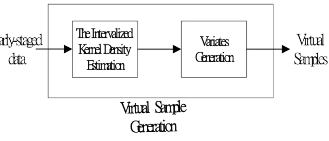
Figure 3.1 Virtual Sample Generation in the learning process contains two steps : the Intervalized Kernel Density Estimation step and the Variates Generation step.

The reason of poor learning quality from small data sets is the lack of information about the population. Theoretically, since the current training data are unrepresentative it is necessary to collect a big number of data in an unstable environment for covering all possible situations. Virtual Sample Generation (VSG) is a direct way to overcome this difficulty. It contains two steps in our study, shown in Figure 3.1, step 1: The Intervalized Kernel Density Estimation, and step 2: Variate Generation. The procedure of VSG will be described in the following.

3.1.1 Intervalized Density Estimation (IDE)

Mathematically, small data set learning cannot achieve high accuracies no matter what kind of learning machine is employed. To conquer it, we believe that realizing data behavior is the beginning step making the

sample size problem less influential. For instance, if we have found that the small set of data possessing a normal distribution, we could generate more data from the normal density function to expand the size of the database for a stable learning. Therefore, Density Estimation is thought an effective approach to lift up the learning accuracy in small sample learning. Along with the conceptual strategy, a special technique---Intervalization is proposed as a part of the method to improve the estimation task.

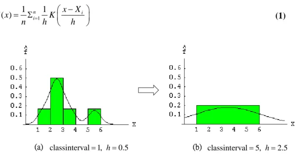
One of the problems in small sample learning using Density Estimation is about the rough estimate. Figure 3.2 shows the poor estimate resulted from few samples. In Figure 3.2(a), the twin-modal curve is an estimate, by kernel methods, of the underlying density using six samples. The original data were classed into 4 bines. If all the six samples belong to 1 bin like that in

(7)

Figure 3.2(b), the uni-modal curve can otherwise be the estimate. Since we have little message about these six samples to believe that they are distributed as a multi-modal distribution, the basic function of intervalization is to systematically fit the data to determine the underlying distribution. In fact, the process of intervalizing data is done through applying kernel methods, and the final number of bins is not always a constant. In general, consider the twin-modal curve in Figure 3.2(a), if these two peaks are located very close to each other, the original data are thought distributed in a uni-modal density, such as that in Figure 3.2(b). On the contrary, if peaks are located far apart from each other, the density might have the shape of multi-modal. For detailed explanation, ponder another example that Figure 3.3(a) is a histogram containing 10 data with class interval equal to 1. Since six of the data on the left are located so close that they can be distributed in a uni-modal density after enlarging the class interval from 1 to 2 (Figure 3.3(b)), or from 1 to 5 (Figure 3.3(c)). Consequently, the point reveals that the ordinary kernel estimator, Function (1), counts on a smoothing parameter h whereas the intervalized kernel estimator concentrates on the determining of the bin number and the scale of class interval. Although h and the scale of class interval have a proportional relationship, they make

different influences to the ordinary and intervalized kernel estimators.

In Figure 3.3(b)(c), the h or h′ is fixed across the left six samples so the ordinary estimator can work well. However, in Figure 3.3(b), the drawback of the ordinary estimator appears while the data are widely distributed and the intervalized one (Figure 3.3(c)) shapes more reasonably. In other words, intervalization provides a mechanism for choosing the number of bins, which can have various sizes. Following this viewpoint, we proposed an intervalized density estimator as formulated in Function (2). In this refined form, we allow for m

kinds of kernel functions, K1, ,K , and m different smoothing parameters, h₁, ,h . _m

Each pair of (K ,_i h ) is corresponding to a _i

set with n data. i

The complete general form of the intervalized multivariate kernel estimator can be procured by modifying from the traditional density estimator (Silverman, 1990) as interpreted in the followings. Given that Χ =( ,x₁ ,x_p) is a data vector of

p-dimension for an observation and its

elements are divided into two parts: the mutually independent variable vector

1

( , , )

I x xk

Χ = , and the correlated variable vector Χ =_D (x_k₊₁, ,x_p). Since x₁, ,x _k

(8)

(a) classinterval 1,= h=0.5 (b) classinterval 5,= h=2.5

Figure 3.2(a)(b). Directly using kernel methods can lead to a poor estimate.

(a) classinterval 1=

(b) classinterval=2, h=1 (c) classinterval=2, h′=1 classinterval=5, h′′=2.5

Figure 3.3. (a) is the histogram of 10 data with class interval equal to 1.

(c) with varied smoothing parameters that fit well than the fixed ones of (b).

1 1 1 ˆ ( ) n i i x X f x K n = h h − ⎛ ⎞ = Σ _⎜ _⎟ ⎝ ⎠ (1) 1 1 1 1 ˆ ( ) m ni j i j i i i x X f x K n = = h h − ⎛ ⎞ = Σ Σ _⎜ _⎟ ⎝ ⎠ where n= Σm_i₌₁n_i. (2)

(9)

are mutually independent, the corresponding joint probability density estimator, g xˆ ( ,1 ,xk), can be rewritten as the product of each marginal probability density estimator, Π_tk₌₁f xˆ ( )_t _t . For the correlated part, x_k₊₁, ,x_p, we can regard them as a vector Χ_D and apply the intervalized density estimator, Function (2), to it. For multivariate cases, each smoothing parameter extends to a p-dimension vector,

P i

h , and Function (3) is the complete

general form of an intervalized multivariate kernel density estimator.

3.1.2 Variate Generation

Virtual Sample Generation is a direct way to overcome the difficulty of small sample set learning, since the current data provide prior information about its distribution and the prior information are always bounded by the data size. Therefore, we propose the intervalized kernel density estimator for small data sets, and it is used in the virtual data generalizing work.

Random Variate Generation has an inverse process comparing with that of Density Estimation. As mentioned before, Density Estimation estimates the underlying density or guesses the true distribution for a given data set, whereas Random Variate Generation produces a desired number of samples from a determined density. ˆ ( ) f Χ =gˆ (Χ_I)lˆ(Χ _D) where Χ = Χ Χ( _I, _D), 1 ( , , ) I x xk Χ = , Χ =D (xk+1, ,xp) 1, , k

x x are mutually independent, x_k₊₁, ,x_p are correlated.

gˆ (ΧI) =g xˆ ( ,1 ,xk) 1ˆ ( )

k t= f xt t

= Π ,

the estimator of joint density g x( ,1 ,xk),

(3) ˆ ( ) 1 m₁ ni₁ 1 t t j t i j i i i x X f x K n = = h h − ⎛ ⎞ = Σ Σ _⎜ _⎟ ⎝ ⎠,

the estimator of density f x , ( )_t

ˆ(l Χ_D) =l xˆ( _k₊₁, ,x_p) 1 _im₁ n_j ₁ 1_p _i D j i i X K n = = h h Χ − ⎛ ⎞ = Σ Σ _⎜ _⎟ ⎝ ⎠,

the estimator of joint density l x( _k₊₁, ,x_p). h_ip =( ,h_i , )h_i ,

m₁ i i

(10)

Simulation is believed a useful approach in Random Variate Generation, such as Markov Chain Monte Carlo Method, it has been used widely for generating a random vector to obtain statistically reliable results. Since we have provided the desired density information in the first step, the Gibbs sampling algorithm (Gelfand & Smith, 1990) will be subsequently employed for the stochastic generation. The main content of the second step is to gain a set of time-dependent manufacturing virtual data. The Gibbs sampler involves in the use of posterior probability that will be discussed in details in the followings.

3.2 Bayesian Application

Here, we define an unconfirmed knowledge as a hypothesis, h, with the probability, P h , computed from the ( ) current data. Bayesian learning is a probabilistic reasoning process through the posterior probability, P h D , computed ( | ) from the following data, D. In other words,

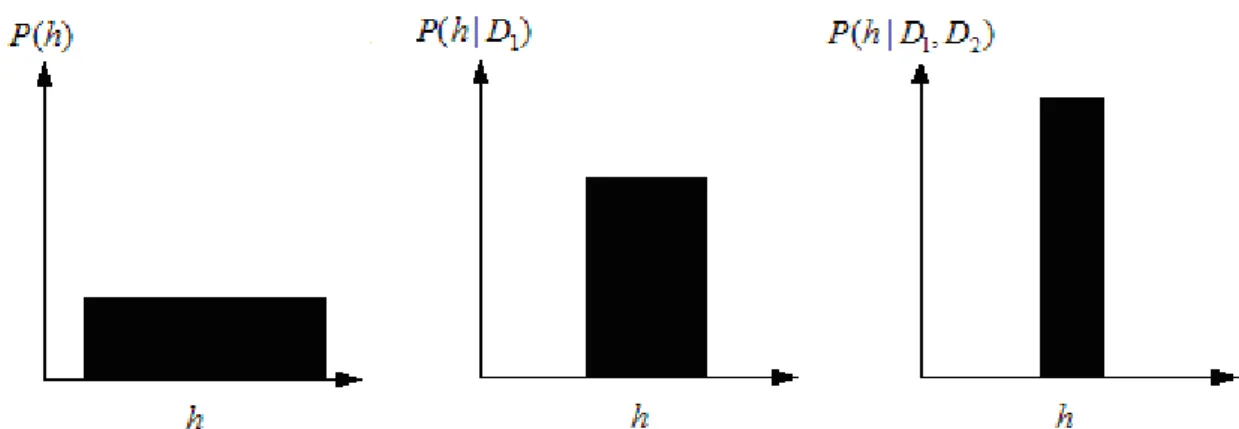
probability measures the degree of belief and the next data corrects the possibility by its impact on P h D . Therefore, Bayesian ( | ) learning has the ability of self-correction. However, we still have to check two important points on the preliminary of Bayesian learning in practical work. As shown in Figure 3.4, the rectangle in the left

is the original probability density of the hypothesis, ( )P h , and a following data, D₁, collected from the manufacturing process, which enhances P h D( | ₁) with its consistent part of P h( ). Then, the next data

2

D will do the same enhancement to minimize the posterior probabilities of inconsistent hypotheses.

First, in the process, determination of prior probabilities is needed in Bayesian learning whereas other methods are not. Without the prior probability, there is no information to help computing the posterior probabilities. Fortunately, the early-staged learning in the practical cases stats from the few data collected at initial periods. Second, Bayesian learning works only if the true knowledge exists in the hypothesis space, which would hold in a manufacturing system.

In Bayesian learning, the learning process updates the prior probability by itself into posterior probability according to the Bayesian rule. In stochastic sampling, one generates a set of samples of the manufacturing system, which forms the updated posterior probability, and the updated posterior probability is used for prediction or decisions making. Bayesian classifier is an example application for updating posterior probability to conduct prediction, and it’s introduced to the

(11)

Figure 3.4 Evaluation of posterior probability P h D( | 1) and P h D D( | 1, 2) (Mitchell, 1997). B E D A C

Figure 3.5 A hypothetical Bayesian network structure (Chen, 2001).

research for decisions making, Bayesian network (BN).

3.2.1 Gibbs Sampler

Gibbs sampler is a kind of Monte Carlo Markov Chain (MCMC) sampling methods, which can be used to indirectly obtain new data or samples from a population following a complex joint distribution. The procedure is unlike the approaches mentioned in section 3.1 with direct generating. However, Gibbs sampler requires the information of prior and posterior probabilities of desired

data (means manufacturing data in our case), which can be provided by IDE.

To further explain the indirect procedure, given a set of given data at early stages,(X₁0,X₂0, ,X_k0), one can findX₁1~

0 0 1 2 ( | , , _k) P X X X , 1 0 0 0 2 ~ ( 2| 1, 3, , k) X P X X X X , 1 0 0 0 0 3 ~ ( 3| 1, 2, 4, , k) X P X X X X X till X1k ~ 0 0 0 1 2 1 ( _k| , , , _k ) P X X X X ₋ with the

assumption that these k distribution exist. After i iterations, the process will reach

1 2

(12)

real distribution, (X1,X2, ,Xk). When sample size, k, is large, this may need a lot of time to gain the convergence (Gelfand & Smith, 1990). Fortunately, k is hardly large in the early stages.

3.2.2 Bayesian Network (BN)

Bayesian network, first presented by Pearl in 1998, utilizes the relationships among the variables to conduct Bayesian analysis for learning. In general, a BN describes the probability distribution over a set of variables, (X1, X2, ,Xk) , and consists of the following parts: 1) A graphical-directed network, containing no-directed cycles, that represents the conditional independence about variables. 2) A set of local probability distributions corresponding to each variable.

As an example, given a database of a manufacturing system and several arbitrarily selected interesting variables, { , , , , }A B C D E , where A represents the

arrival rate of parts, and B represents the buffer size, etc. According to the conditional probability, a hypothetical BN structure is established as shown in Figure 3.5. This graphical network represents the causal relationships among these five variables. For example, in the sequential connection C→ →D E , the event of

variable C influences the event of variable

D, and in turn influences the event of

variable E. If the information about variable

D is determined, the event of variable C will

not influence the event of variable E in terms of probability dependency. That is the concept of conditional independence. The conditionally independent property is an important character and is used for saving more computational cost in BN. To explain further, let , ,C D E be three discrete-valued random variables, where E is conditional independent of C given D. If the distribution of E is independent of the value of C given a value of D, which is

described as ( | , ) ( | ) P E=e C=c D=d =P E=e D=d or in abbreviated form ( | ) ( | ) P E CD =P E D . A BN represents the joint probability distribution by specifying a set of conditional impendence assumptions with essentially sets of local conditional probabilities. Therefore, we are sure about two points in every node of a given BN. First, the network arc would show the conditional independence of the current node form non-adjacent nodes in a BN. Second, a conditional probability distribution hass assigned to each variable. In fact, we can find the causal relationship directly from the graphical structure of BN. For example, we say that C and B cause D. This is another attractive feature.

(13)

Since the BN is an inferable structure, it is useful to use it to conduct the inference about the target variables with the observed values of other variables. Except that the inference process is to derive the posterior distribution rather than assigning a possible value to the target variable. A BN can be used to compute the posterior distribution for any subset of network variables given obtained values and distributions of any subset of the remaining variables. Russell et al. (1995) propose a gradient-based approach to train the BN structure. BN can be trained with a gradient descent algorithm such as the training method for ANNs. The main concept of the gradient-based training of BN is to maximize the probability of data

D presented under hypothesis h, (P D h | ) by following the gradient of ln (P D h | ) with respect to the parameters that define the conditional distribution of nodes in a BN. In ANNs’, the parameters representing the connected weights of any two adjacent nodes, are regarded as a kind of connecting intensities. This is similar to the conditional probabilities corresponding to each arc.

3.2.3 Dynamic Bayesian Network (DBN)

Often a Bayesian network is constructed by combining a priori knowledge, perhaps from an expert in a particular domain, with conditional independences between the

variables and a set of observations (This priori knowledge can be elicited from the expert by asking questions regarding causality.) For instance, a variable that has a direct causal effect on another variable will be its parent in the network since temporal order specifies the direction of causality, and plays an important role in the design of dynamic Bayesian networks. In time series modeling, we observe the values of certain variables at different points of time, such as the case in a manufacturing process. The assumption that an event can cause another event in the future, simplifies the design of Bayesian networks for time series: directed arcs should flow forward in terms of time. When assigning a time index t to each variable, one of the simplest causal models for a sequence of data { ,Y₁ …,Y_T} is the first-order Markov model, in which only the previous one affects each variable as shown in Figure 3.6 described as P Y( ,₁ …,Y_T)

1 2 1

( ) ( | )

P Y P Y Y

= P Y( _T |Y_T₋₁)

Ghahramani (1998) developed a new BN structure representing a high-order Markov model and directly displaying the dependencies over more than one time step. However, we do not at this moment attempt to apply the complicated structure in the early-staged learning model until the learning capability of first-order structure is found limited.

(14)

Figure 3.6 a Bayesian network representing the first-order Markov model.

4. The Experimental Study

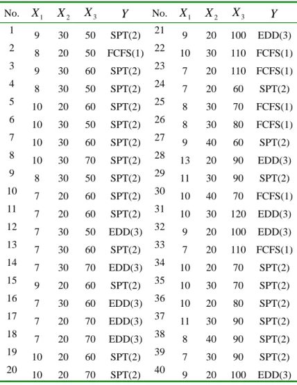
The following data, presented in Table 4.1, are an example set from a flexible manufacturing system (Li et al, 2003). There are four variables in this simulated system, where X₁ represents the buffer size, X₂

represents the arrival rate of parts, X ₃

represents the speed of automobile general motors, and Y is the best scheduling rule.

They consist of three scheduling rules: FCFS means the rule of “First come, first served” coded as 1; SPT means the rule of Short Processing Time coded as 2; and EDD means the rule of Earlier Due Date coded as 3. We try to acquire a concept from the training data for future use. (The full study with the manufacturing model, situations, and complete analysis can be found in Li et al (2003). But one need not review the full manufacturing system to understand this study.) This small data set contains 40 raw-data from the FMS.

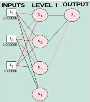
The task of this supervised learning process will employ the common artificial neural network, Back Propagation Network (BPN), to find scheduling knowledge, the

Figure 4.1 A 3-4-1 network structure with 3 input units, 4 computational

units located at a hidden layer and 1 output unit.

relationship between these three controlling factors (X₁, X₂, X ) on the production ₃

line and the scheduling rule (Y). The

corresponding network has three input units, four computational units located at one hidden layer and one output unit; that is, a 3-4-1 structure, since the more complicated a structure is, the more sample complexity it spends. It is expected that large network structures always have a huge amount of connected weights needed sufficient enough data for training for a good performance.

(15)

Table 4.1 The whole scheduling data set. (Chen, 2000) No. X1 X2 X3 Y No. X1 X2 X3 Y 1 9 30 50 SPT(2) 21 9 20 100 EDD(3) 2 _{8 20 50} _FCFS(1) 22 ₁₀ ₃₀ ₁₁₀ _FCFS(1) 3 _{9 30 60} _SPT(2) 23 _{7 20} ₁₁₀ _FCFS(1) 4 _{8 30 50} _SPT(2) 24 _{7 20} ₆₀ _SPT(2) 5 _{10 20 60} _SPT(2) 25 _{8 30} ₇₀ _FCFS(1) 6 10 30 50 SPT(2) 26 8 30 80 FCFS(1) 7 10 30 60 SPT(2) 27 9 40 60 SPT(2) 8 10 30 70 SPT(2) 28 13 20 90 EDD(3) 9 _{8 30 50} _SPT(2) 29 ₁₁ ₃₀ ₉₀ _SPT(2) 10 _{7 20 60} _SPT(2) 30 ₁₀ ₄₀ ₇₀ _FCFS(1) 11 _{7 20 60} _SPT(2) 31 ₁₀ ₃₀ ₁₂₀ _EDD(3) 12 _{7 30 50} _EDD(3) 32 _{9 20} ₁₀₀ _EDD(3) 13 _{7 30 60} _SPT(2) 33 _{7 20} ₁₁₀ _FCFS(1) 14 7 30 70 EDD(3) 34 10 20 70 SPT(2) 15 9 20 60 SPT(2) 35 10 30 70 SPT(2) 16 7 30 60 EDD(3) 36 10 20 80 SPT(2) 17 _{7 20 70} _EDD(3) 37 ₁₁ ₃₀ ₉₀ _SPT(2) 18 _{7 20 70} _EDD(3) 38 _{8 40} ₉₀ _SPT(2) 19 _{10 20 60} _SPT(2) 39 _{7 30} ₉₀ _SPT(2) 20 _{10 20 70} _SPT(2) 40 _{9 20} ₁₀₀ _EDD(3)

The output unit has linear activation while the computational units in only one hidden layer have sigmoid ones given by

( ) 1 [1 exp( )]

f x = + −x .

To show the poor learning performance

from the small data set, we randomly split the whole data set into two parts—training and testing sets, for various sizes. The size of the training set is 5 at first and increases by 5, each time to be 10, 15, 20, 25, 30, while the size of corresponding testing sets

Table 4.2 The accuracies of classification with variant sample sizes.

Sizes of training set Size of testing set Average accuracies 5 35 0.26 10 30 0.33 15 25 0.34 20 20 0.43 25 15 0.45

30 10 0.50 Figure 4.2 The classification accuracy rises as the size of training data increases.

(16)

are, in the remainders, 35, 30, 25, 20, 15, 10 decreasingly. For each paired size of data sets, we made 10 trials and obtained the average accuracies. As shown in Table 4.2, the learning results present low classification accuracies before using virtual samples generated from IKDE. Insufficient data and an unstable production process can be the main explanations of this phenomenon.

Naturally, in the early manufacturing stages, the obtained training data size is too small to cover all possible situations in the manufacturing system. For an extreme example of a 5-data training set, the training data sometimes contain only one or two kinds of scheduling data because it is randomly selected from 40 data consisted of 7 FCFS, 23 SPT and 10 EDD.

The corresponding average testing accuracy is obviously low (26%, in Table 4.2). Even though the training set contains three kinds of scheduling data such as the 10-data cases, 15-data case etc., the relatively insufficient information still reflects poor learning performance.

4.1 Virtual Sample Generation

To expedite the forming of scheduling knowledge, we are now using the proposed small-data-set learning approach to build it up as explained in the following, which includes two works: 1. Virtual Sample

Generation and 2. Learning scheduling knowledge.

4.1.1 Applying Intervalized Kernel Density Estimation

Here we apply the Intervalized Kernel Density Estimation method (Function (10)) to find the approximate density estimators of the current data. There are 3 variables,

1

X X₂ and X3, and 1 class variable, Y.

Therefore, the joint conditional probability density estimators for each class are formed as f x x xˆ ( , , |₁ ₂ ₃ Y = y) where y=1, 2, 3 . Assuming X1, X2, and X3 are mutually

independent in the manufacturing system, the joint conditional probability density estimator can factor into 3 independent conditional probability density estimators:

1 ˆ ( | )

f x Y =y , f xˆ ( |2 Y =y), and f xˆ ( |3 Y =y).

Thus, Function (6) is applied to these uni-variate cases.

On the basis of the statistical independent property, we derive

1 2 3 ˆ ( , , | )

f x x x Y =y from the product of its’ uni-variate conditional density estimators:

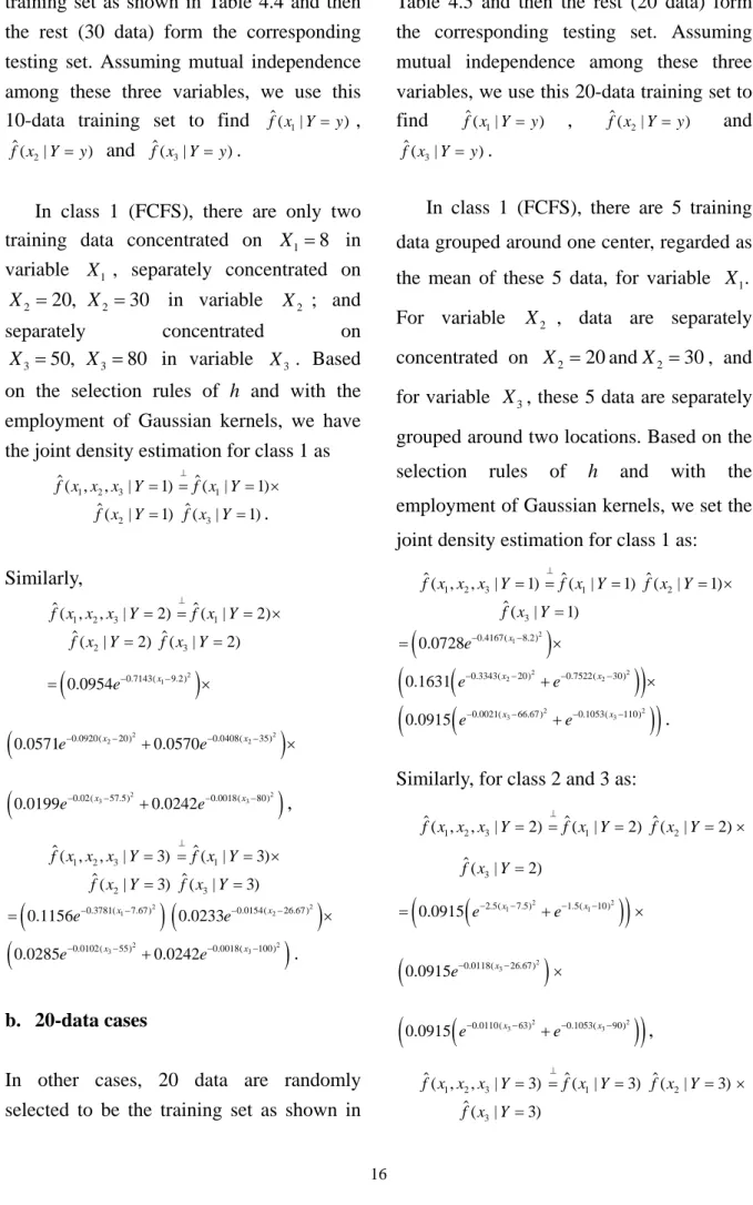
a. 10-data cases

(17)

training set as shown in Table 4.4 and then the rest (30 data) form the corresponding testing set. Assuming mutual independence among these three variables, we use this 10-data training set to find f x Yˆ ( |₁ = y) ,

2 ˆ ( | )

f x Y =y and f xˆ ( |3 Y =y).

In class 1 (FCFS), there are only two training data concentrated on X₁ =8 in variable X₁ , separately concentrated on

2 20, 2 30

X = X = in variable X₂ ; and

separately concentrated on

3 50, 3 80

X = X = in variable X₃. Based on the selection rules of h and with the

employment of Gaussian kernels, we have the joint density estimation for class 1 as

3 3 0.0102( 55) 0.0018( 100) 0.0285_e− x− +0.0242_e− x− _. b. 20-data cases

In other cases, 20 data are randomly selected to be the training set as shown in

Table 4.5 and then the rest (20 data) form the corresponding testing set. Assuming mutual independence among these three variables, we use this 20-data training set to find f x Yˆ ( |₁ =y) , f xˆ ( |2 Y =y) and

3 ˆ ( | ) f x Y =y .

In class 1 (FCFS), there are 5 training data grouped around one center, regarded as the mean of these 5 data, for variable X1.

For variable X2 , data are separately

concentrated on X₂ =20andX₂ =30, and for variable X , these 5 data are separately ₃

grouped around two locations. Based on the

selection rules of h and with the

employment of Gaussian kernels, we set the joint density estimation for class 1 as:

(

)

(

)

(

)

(

)

(

)

2 2 1 1 2 2 2 2 2 2 3 3 0.25( 8) 0.2988( 13) 0.3343( 20) 0.0836( 30) 0.0263( 50) 0.01( 95) 0.0915 0.3084 0.1631 0.0915 . x x x x x x e e e e e e − − − − − − − − − − − − = + × + × +

Although we have the joint conditional density estimators, statistical independence helps us to generate every conditional uni-variate ( X1|Y =1, X2|Y =1, ) and

combine them rather than generate multivariate

((X1,X2,X3|Y =1), (X1,X2,X3|Y =2), ).

The final estimators shown above (in 10-data cases and 20-data cases) are just the results obtained from one randomly selected training set for demonstrating the process of IKDE. In this study, we have randomly selected the training samples (set) for each of these two kinds of cases over 10 times (runs).

Table 4.4 An example of a 10-data training set by random selection. 1 X X₂ X3 Y 8 20 50 1 8 30 80 1 9 40 60 2 10 20 60 2 9 20 60 2 8 30 50 2 10 20 80 2 7 30 50 3 9 20 100 3 7 30 60 3

Table 4.5 An example of a 20-data training set by random selection. 1 X X₂ X3 Y 8 20 50 1 10 30 110 1 7 20 110 1 8 30 80 1 8 30 70 1 10 20 60 2 11 30 90 2 7 30 60 2 8 30 50 2 9 40 60 2 10 20 70 2 7 30 90 2 10 30 70 2 7 20 60 2 10 20 70 2 10 30 70 2 7 20 60 2 13 20 90 3 9 20 100 3 7 30 50 3 4.1.2 Variate Generation

Following the demonstration of intervalized kernel density estimation, variate generation is the second step in virtual sample generation. For the Gaussian kernel function employed in this case, we apply the modified polar method to the intervalized kernel density estimator. In addition, since we have assumed the independence among these three variables, respective generation for each variable in each class can simplify the processes of whole variate generation. For example, when the generation of random vector

1 2 3

(X ,X ,X |Y =1) is concerned, one can generate random variates ( X1|Y =1 ),

(19)

of samples individually, and combine them to form a set of the desired random vector

1 2 3

(X ,X ,X |Y=1). We are interested in the variation of learning accuracy with increasing virtual samples. Therefore, there are 20, 30, 40, 50, 60 virtual samples, respectively, generated from the joint density estimator built by IKDE in 10-data cases for training the 3-4-1 BPN network structure as mentioned before. In 20-data cases, we generated 30, 40, 50, 60 virtual samples, respectively, for training the same network structure as well.

4.2 Learning with the Virtual Samples

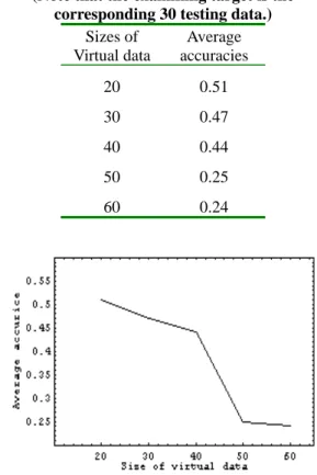
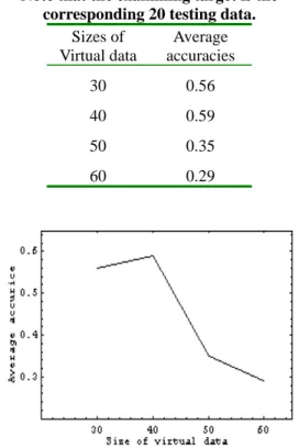
To verify the improvement of learning from small data sets using the virtual sample generation, we regarded the corresponding testing sets of the two demonstrating cases (a and b) as the examination target. For these two cases, each has 30 and 20 testing data, individually and the learning accuracies are shown in Table 4.6 and Table 4.7. It is found that the average accuracy rises at the start of using virtual training data. For 10-data cases, the average accuracy of the training result from its original 10-data set is 0.33 (Table 4.2) and rises to 0.51 after using 20 virtual data for training. As the size of virtual data increases, the average learning accuracy decreases (Figure 4.3). The same situation occurs in 20-data cases. Table 4.2 shows that average accuracy is 0.43 when learning with the original 20 training data. As we use a larger

size of virtual data for training, the average accuracy increases to 0.56, even 0.59 (Table

4.7). However, the more virtual data applied to training, the worse the performance achieved.

Both of the learning results, shown in Table 4.6 and 4.7, from virtual training samples reveal two interesting conclusions. First, using virtual data generated through IKDE does help improve the learning performance. Second, the average accuracy decreases as the number of virtual training data increases. This may be caused by the over-lapping effect. We shall discuss the possible reason for this phenomenon in the following section.

Table 4.6 The average accuracies of learning results from various sizes of virtual training data.

(Note that the examining target is the corresponding 30 testing data.)

Sizes of Virtual data Average accuracies 20 0.51 30 0.47 40 0.44 50 0.25 60 0.24

Figure 4.3 The average accuracies rise at the start of using virtual data for training and then have a

decreasing trend. Note that the examining target is the corresponding 30 testing data.

(20)

Table 4.7 The average accuracies of learning results from various sizes of virtual training data.

Note that the examining target is the corresponding 20 testing data.

Sizes of Virtual data Average accuracies 30 0.56 40 0.59 50 0.35 60 0.29

Figure 4.4 The average accuracies rise at the start of using virtual data for training and then have a sharply decreasing trend. Note that the examining

target is the corresponding 20 testing data.

4.3 Conclusion

We have experimented with the FMS data in a manufacturing system for illustrating and verifying the performance of the proposed strategy to improve the small data sets learning. A set of only 40 scheduling data is available for the experiment. We try to acquire the scheduling knowledge from the 10 or 20 training data of random selection by formulating the intervalized kernel density estimators and generate the virtual training set. The generated virtual data obviously raise the testing accuracies when examining the results (Table 4.6 and 4.7, Figure 4.3 and 4.4).

Virtual sample generation not only produces data resembling the original training data set but also explore the possible domains for attributes of the manufacturing system: the buffer size (X Y₁| ), the arrival rate of parts (X2|Y),

and the speed of automobile generator motors (X3|Y ). We believe that this extra

sample information created by the study help the learning tool to improve the scheduling rules for the manufacturing system.

5. Discussion

Virtual Sample Generation using the Intervalized Kernel Density Estimation overcomes the difficulty of learning with insufficient data. This is because that KDE emphasizes the estimation of every datum while IKDE concentrates on the kernel center locations. We believe that generating more resembling samples from the small training set makes the learning tools perform well. Our proposed method is based on kernel density estimation but there is still a difficulty in applying it to the system with nominal variables. Also, a system with high variance between stages, this research may have chance to show less effective prediction. Virtual sample generation for nominal variables can be a new focus of our future study.

In our experience, however, the determination of smoothing parameters, h’s,

(21)

could influence the quality of virtual sample generation. In the experimental study, we set different h’s for some estimators because

the shapes of these data distributing are different from one another. In practice, the setting of h should be based on the users’

background knowledge. From a theoretical point of view, however, we suggest a referring parameter—the standard deviation of data belonging to each grouped data as the index for choosing h’s.

When formulating the conditional intervalized kernel density estimators of

1 2 3

(X ,X ,X |Y= y) , we have assumed the three variables are independent of one another for simplifying the works. Nevertheless, in future studies, the relationship between the variables, independent or correlated, should be considered as an important factor affecting the quality of virtual data. Note that a suggestion is that one can generate random vectors (X1,X2,X3|Y =y) without the

independent assumption. For example, suppose that (X1,X2|Y =y) is following a

bivariate normal distribution with its mean vector (µ µ1, 2|Y= y) , variance vector

2 2 1 2

(σ σ, |Y = y) , and the correlation coefficient ρ . That is, there must be a linear relationship between X1|Y =y and

2|

X Y =y according to the property of bivariate normal distributions. After generating variates of X1|Y = y, we can

have variates of X2|Y =y through linearly

transferring (Function (14)) instead of generating it directly. In other words, we can obtain a set of variates of one variable

through the transforming relationship with other variables.

Another issue for future studies is the size of virtual data. In this scheduling case, we train the BPN network with increasing virtual samples and the learning accuracy decreases as the number of virtual samples increased. To explain this problem, as presented in Figure 5.1, we consider that the virtual data are not all sampled from the data population as the number increases. But this question concerning the size of virtual samples is worthy of future research.

Data Population

Virtual data Small data set

Figure 5.1 The relationship among the population, obtained data and virtual

data.

Reference

Amaratunga, D., 1999. Searching for the right sample size. American Statistician, 53, 52-55.

Eggermont, P. P. B., Lariccia, V. N., 1997. Nonlinearly smoothed EM density estimation with automated smoothing parameter selection for nonparametric deconvolution problems, Journal of the American Statistical Association, 92,

2| 2| 2| 1| 1| 1| ( ) Y y Y y Y y Y y Y y Y y X µ ρσ X µ σ = = = = = = = + − ₍₁₄₎

(22)

1451-1458.

Gangopadhyay, A. K., Cheung, K. N., 2002. Bayesian approach to the choice of smoothing parameter in kernel density estimation, Nonparametric Statistics, 14(6), 655-664.

Gu, B., Liu B., Hu F., Liu, H., 2001. Efficiently Determining the Starting Sample Size for Progressive Sampling, Lecture Notes in Computer Science, 2167, 192-201.

Gu, C., 1998. Model indexing and smoothing parameter selection in nonparametric function estimation, Statistica Sinica, 8, 607-623.

Hall, P., Kang, K. H., 2001. Bootstrapping nonparametric density estimators with empirically chosen bandwidths, Annals of Statistics, 29(5), 1443-1468.

Hastie, T., Tibshirani, R., Friedman, J., 2001. The elements of statistical learning—Data mining, inference and prediction. Springer-Verlag, New York. Hernández-Aguirre, A., Koutsougeras, C.,

Buckles, B.P., 2002. Sample Complexity for Function Learning Tasks. Lecture Notes in Computer Science, 2313, 267-271.

Kendall, M.G., Stuart A., 1973. The Advanced Theory of Statistics, Volume 2, 3rd Edition. Griffin, London.

Lanouette, R., Thibault, J., Valade J. L., 1999. Process modeling with neural network using small experimental datasets. Computers and Chemical Engineering, 23, 1167-1176.

Li, D. C., Chen, L. S., Lin, Y. S., 2003. Using Functional Virtual Population as an Assistance to Learn Scheduling Knowledge. International Journal of Production Researches, 41(17),

4011-4024.

Niyogi, P., Girosi, F., Tomaso, P., 1998. Incorporating Prior Information in Machine Learning by Creating Virtual Examples. Proceeding of the IEEE, 86(11), 275-298.

Onisko, A., Druzdzel, M. J., Wasyluk, H., 2001. Learning Bayesian network parameters from small data sets: application of Noisy-OR gates. International Journal of Approximate Reasoning, 27, 165-182.

Parzen, E.,1962. On estimation of a probability density function and mode. Annals of Mathematical Statistics, 33, 1065-1076.

Rosenblatt, M., 1956. Remarks on some nonparametric estimates of a density estimation. Annals of Mathematical Statistics, 27, 832-837.

Ross, S. M., 1996. Simulation/Second Edition. Academic Press, San Diego.

(23)

應用貝氏學習理論獲取彈性製造系統初期之排程知識

行政院國家科學委員會專題研究計畫 成果報告