Nonlinear stability analysis of the thin pseudoplastic liquid film flowing down along a vertical wall

Nonlinear stability analysis of the thin pseudoplastic liquid film flowing down along a vertical wall

Po-Jen Cheng

Department of Mechanical Engineering, Far-East College, Tainan, Taiwan, Republic of China

Cha’o-Kuang Chen

^a)

and Hsin-Yi Lai

Department of Mechanical Engineering, National Cheng-Kung University, Tainan, Taiwan, Republic of China

共Received 16 October 2000; accepted for publication 5 February 2001兲

This article investigates the weakly nonlinear stability theory of a thin pseudoplastic liquid film flowing down on a vertical wall. The long-wave perturbation method is employed to solve for generalized nonlinear kinematic equation with free film interface. The normal mode approach is used to compute the linear stability solution for the film flow. The method of multiple scales is then used to obtain the weak nonlinear dynamics of the film flow for stability analysis. It is shown that the necessary condition for the existence of such a solution is governed by the Ginzburg–Landau equation. The modeling results indicate that both subcritical instability and supercritical stability conditions are possible to occur in a pseudoplastic film flow system. The results also reveal that the pseudoplastic liquid film flows are less stable than Newtonian’s as traveling down along the vertical wall. The degree of instability in the film flow is further intensified by decreasing the flow index n.

© 2001 American Institute of Physics. 关DOI: 10.1063/1.1359152兴

I. INTRODUCTION

The stability of a film flow is a research subject of great importance commonly needed in mechanical, chemical, and nuclear engineering industries for various applications in- cluding the process of paint finishing, the process of laser cutting, and heavy casting production processes. It is known that macroscopic instabilities can cause disastrous conditions to fluid flow. It is thus highly desirable to understand the underlying flow characteristics and associated time- dependent properties so that suitable conditions for homoge- neous film growth can be developed for various industrial applications.

The problem of the stability of the laminar flow of an ordinary viscous liquid film flowing down an inclined plane under gravity was first formulated and solved numerically by Yih.

¹

The transition mechanism from laminar flow to turbu- lent flow was elegantly explained by the Landau equation.

²

That shed a light for later development on nonlinear film stability. The Landau equation was later rederived by Stuart

³

using the disturbed energy balance equation along with Rey- nolds stresses. Benjamin

⁴

and Yih

⁵

formulated the disturbed wave equation of free flow surface. The flow stability of the long disturbed wave was carefully studied and some charac- teristics of the flow stability on an inclined plane are ob- served. These include 共1兲 the flow that is disturbed by a longer wave is less stable than that disturbed by a shorter wave; 共2兲 the film flow is less stable as the inclined angle increases; 共3兲 the film flowing down a vertical plate becomes unstable as the critical Reynolds number becomes nearly zero; 共4兲 the film flow becomes relatively stable as the sur- face tension of the film increases; 共5兲 the velocity of the

unstable long disturbed wave is approximately twice of the wave velocity traveling on the free surface.

Benney

⁶

investigated the nonlinear evolution equation of free surface by using the method of small parameters. The solutions thus obtained can be used to predict nonlinear in- stability. However, the solutions cannot be used to predict supercritical stability since the influence of surface tension is not considered in the analysis of the small-parameter method. The effect of surface tension was realized by many researchers as one of the necessary conditions that will lead to the solution of supercritical stability. Lin,

⁷

Nakaya,

⁸

and Krishna and Lin

⁹

considered the significance of surface ten- sion and treated it in terms of zeroth order terms in later studies. Pumir et al.

¹⁰

further included the effect of surface tension into the film flow model and solved for the solitary wave solutions. Hwang and Weng

¹¹

showed that the condi- tions of both supercritical stability and subcritical instability are possible to occur for a liquid film flow system. An ex- tensive review on the stability of falling liquid can be re- ferred to Chang.

¹²

Renardy and Sun

¹³

and Tsai et al.

¹⁴

have done the work on both linear and nonlinear stability analysis of a fluid film flowing down along an inclined or vertical plate. Detailed flow analysis is indeed of great importance in the development of stability theory for characterizing various flow film conditions.

A vast majority of studies on thin-film flow problems were devoted to the stability analysis of Newtonian fluids.

The film flow of non-Newtonian fluids attracted less atten- tion in the past. The rheological behaviors of fluids during the plastic manufacture, the lubrication of bearings, or the glue in biological chemistry do not obey the Newtonian pos- tulate. In recent years, the microstructure of fluid flows has emerged as a research subject of great interest to many re-

a兲Electronic mail: ckchen@mail.ncku.edu.tw

8238

0021-8979/2001/89(12)/8238/9/$18.00 © 2001 American Institute of Physics

searchers. Hung et al.

¹⁵

employed the method of nonlinear analysis to study the stability of thin micropolar liquid films flowing down along a vertical plate. The results of their study indicated that the micropolar parameter plays an im- portant role in stabilizing a film flow. The viscoelastic fluid, a subclass of microstructure flows, exhibits a great deal of influence on the normal and shear stresses in flow films. The stability problem of a falling film of viscoelastic fluid has been studied by Gupta

¹⁶

who considered the stability of a small-amplitude falling fluid of second order. The long wavelength disturbance is used in the article to conduct a linear stability analysis. After deriving the viscoelastic ana- log of the Orr–Sommerfeld equation with the requisite boundary condition, Gupta pointed out the viscoelastic effect can destabilize the film flow. Cheng et al.

¹⁷

further studied the nonlinear stability analysis of thin viscoelastic liquid film flowing down on a vertical wall. They also demonstrated that the viscoelastic property has a destabilizing effect on the nonlinear film flow system.

In practical applications, pseudoplastic fluids that show shear thinning are widely used in the analysis to characterize the molten polyethylene and polypropylene, and solutions of carboxymethylcellulose 共CMC兲 in water, polyacrylamide in water and glycerin, and aluminum laurate in decalin and m-cresol in various industrial sectors. Almost all polymer solutions and melts that exhibit a shear-rate dependent vis- cosity are pseudoplastic. The polymeric fluid drains much more quickly than the Newtonian fluid when the fluids are allowed to flow out by gravity in the vertical tubes.

¹⁸

The viscosity of the macromolecular fluid appears to be lower in the higher shear rate part of the experiment. For many engi- neering applications, this is the most important characteristic of polymeric fluids. Ng and Mei

¹⁹

studied the roll waves on a shallow layer of mud modeled as a power-law fluid. The results indicated that longer roll waves, with dissipation at the discontinuous fronts, cannot be maintained if the uniform flow is linearly stable, when the fluid is slightly non- Newtonian. However, when the fluid is highly non- Newtonian, very long roll waves may still exist even if the corresponding uniform flow is stable to infinitesimal distur- bances. Hwang et al.

²⁰

studied the linear stability of power- law liquid film flows down an inclined plane by using the integral method. The results reveal that the system will be more unstable when power-law exponent n decreases.

The stability analysis of the pseudoplastic film flow is an interesting research area in both theoretical development and practical applications. So far the weakly nonlinear stability analysis of a thin pseudoplastic liquid film flowing down a vertical wall has not been seriously investigated. However, since the types of stability problems are of great importance in many practical applications, the behavior of a pseudoplas- tic liquid film traveling down along a vertical wall is care- fully studied in this article by employing both linear and nonlinear stability analysis theories. The influence of pseudoplastic property on finite-amplitude equilibrium is studied and characterized mathematically. The sensitivity analysis of the flow index n is also carefully conducted. Sev- eral numerical examples are presented to verify the solutions

and to demonstrate the effectiveness of the proposed model- ing procedure.

II. GENERALIZED KINEMATIC EQUATIONS

Figure 1 shows the configuration of a thin pseudoplastic liquid film flowing down on a vertical wall. The pseudoplas- tic fluid that gives shear thinning to the Ostwald–de Waele model obeys the constitutive equation of state

²¹

␶

i j

⫽⫺p * ␦

i j

⫹2 ␮

n

⌰e

i j

, 共1兲 where ␶

i j

is the stress tensor, e

_{i j}

is the rate-of-strain tensor,

␮

n

is the dynamic viscosity of pseudoplastic flow, p * is the isotropic pressure, and

⌰⫽关2共e

x*^x*

2

⫹e

_y²_*y*

兲⫹4e

x*^y*

2

兴 ^{共n⫺1兲/2}

⫽ 再 ² 冋冉 ^{⳵ ⳵ u x * *} 冊

²

^⫹ 冉 ^{⳵ ⳵ v y * *} 冊

²

册 ^⫹ 冉 ^{⳵ ⳵ v x * * ⫹ ⳵ ⳵ u y * *} 冊

²

冎 ^{共n⫺1兲/2 ,}

共2兲 where u * and v * are the velocity components in x * and y * directions, respectively, and n is the flow index (n ⬍1). The principles of mass and momentum conservation for an iso- thermal incompressible pseudoplastic flow configuration leads one to a set of system governing equations.

²¹

The gov- erning equations can be expressed in terms of Cartesian co- ordinates (x * , y * ) as

⳵ ^u *

⳵ ^x * ^⫹

⳵ ^v *

⳵ ^y * ^{⫽0, 共3兲}

␳ 冉 ^{⳵ ⳵ u t * * ⫹u * ⳵ ⳵ x u * * ⫹v * ⳵ ⳵ y u * *} 冊 ^{⫽ ␳ g ⫹ ⳵␶ ⳵}

^x

^x

^*

^*

^x*

^{⫹ ⳵␶ ⳵}

^y

^y

^*

^*

^x*

^,

共4兲

␳ 冉 ^{⳵ ⳵ v t * * ⫹u * ⳵ ⳵ x v * * ⫹v * ⳵ ⳵ y v * *} 冊 ^{⫽ ⳵␶ ⳵}

^x

^x

^*

^*

^y*

^{⫹ ⳵␶ ⳵}

^y

^y

^*

^*

^y*

^{, 共5兲}

where ␳ is a constant density of the film flow, t * is the time, g is the gravitational acceleration, and the individual stress components are given as

FIG. 1. Schematic diagram of a pseudoplastic thin film flow traveling down along a vertical wall.

␶

x*^x*

⫽⫺p * _⫹2 ␮

n

⌰e

x*^x*

⫽⫺p * _⫹2 ␮

n

再 ² 冋冉 ^{⳵ ⳵ u x * *} 冊

²

^⫹ 冉 ^{⳵ ⳵ v y * *} 冊

²

册

⫹ 冉 ^{⳵ ⳵ v x * * ⫹ ⳵ ⳵ u y * *} 冊

²

冎 ^{共n⫺1兲/2 ⳵ ⳵ x u * * , 共6兲}

␶

y*^y*

⫽⫺p * _⫹2 ␮

n

⌰e

y*^y*

⫽⫺p * _⫹2 ␮

n

再 ² 冋冉 ^{⳵ ⳵ u x * *} 冊

²

^⫹ 冉 ^{⳵ ⳵ v y * *} 冊

²

册

⫹ 冉 ^{⳵ ⳵ v x * * ⫹ ⳵ ⳵ u y * *} 冊

²

冎 ^{共n⫺1兲/2 ⳵ ⳵ y v * * , 共7兲}

␶

x*^y*

⫽ ␶

y*^x*

⫽2 ␮

n

⌰e

x*^y*

⫽ ␮

n

再 ² 冋冉 ^{⳵ ⳵ u x * *} 冊

²

^⫹ 冉 ^{⳵ ⳵ v y * *} 冊

²

册

⫹ 冉 ^{⳵ ⳵ v x * * ⫹ ⳵ ⳵ u y * *} 冊

²

冎 ^{共n⫺1兲/2} 冉 ^{⳵ ⳵ v x * * ⫹ ⳵ ⳵ u y * *} 冊 ^{. 共8兲}

The no-slip boundary conditions on the wall surface at y *

⫽0 are given as

u * _{⫽0, 共9兲}

v * _{⫽0. 共10兲}

The boundary conditions for free surface at y * _⫽h * are de- rived based on the results given by Edwards et al.

²²

The vanishing of shear stress on free surface gives another boundary condition as

⳵ ^h *

⳵ ^x * 冋 ^{1 ⫹} 冉 ^{⳵ ⳵ h x * *} 冊

²

册 ^{⫺1 共 ␶}

^y*y*

^{⫺ ␶}

^x*x*

^兲

⫹ 冋 ^{1 ⫺} 冉 ^{⳵ ⳵ h x * *} 冊

²

册冋 ^{1 ⫹} 冉 ^{⳵ ⳵ h x * *} 冊

²

册 ^{⫺1 ␶}

^x*y*

^{⫽0. 共11兲}

By solving the balance equation in the direction normal to the free surface, the resulting normal stress condition can be expressed as

冋 ^{1 ⫹} 冉 ^{⳵ ⳵ h x * *} 冊

²

册 ^⫺1 冋 ^{2 ␶}

^x*y*

^{⳵ ⳵ x h * * ⫺ ␶}

^y*y*

^{⫺ ␶}

^x*x*

冉 ^{⳵ ⳵ h x * *} 冊

²

册

⫹S * 再 ^{⳵ ⳵}

²

^{x h * *}

²

冋 ^{1 ⫹} 冉 ^{⳵ ⳵ h x * *} 冊

²

册 ^⫺3/2 冎 ^⫽p

^a

^{* . 共12兲}

The kinematic condition that the flow does not travel across a free surface can be given as

⳵ ^h *

⳵ ^t * ^⫹

⳵ ^h *

⳵ ^x * ^u * _⫺v * _{⫽0, 共13兲}

where h * is the local film thickness, p

_a

* is the atmosphere pressure, and S * is the surface tension. The variable that is associated with a superscript ‘‘ * ’’ stands for a dimensional quantity. By introducing a stream function ␸* , the dimen- sional velocity components can be expressed as

u * ⫽ ⳵␸*

⳵ ^y * ^{, v} * ⫽⫺ ⳵␸*

⳵ ^x * ^{. 共14兲}

The dimensionless quantities can also be defined and given as

x ⫽ ␣ ^x * h

₀

* ^{, y ⫽}

y * h

₀

* ^{, t ⫽}

␣ ^u

0

* t * h

₀

* ^{, h ⫽}

h * h

₀

* ^,

␸ ⫽ ␸*

u

₀

* h

₀

* ^{, p ⫽}

p * _⫺p

_a

*

␳ ^u

0

*

²

^Re

ⁿ

^⫽

u

₀

*

²

^⫺n h

₀

*

ⁿ

v

_n

, 共15兲

S ⫽ S *

共2 ^⫺3n

²

^⫹3n⫹2 ␳

ⁿ

^{⫹2 v}

⁴

^g

³ⁿ

^⫺2 兲

^1/

^共n⫹2兲 , ␣ ⫽ 2 ␲ ^h

0

*

␭ , where Re

_n

is the Reynolds number of pseudoplastic flow, ␭ is the perturbed wave length, and ␣ is the dimensionless wave number. h

₀

* is the film thickness of local base flow and u

₀

* is the reference velocity which can be expressed as

u

₀

* _⫽ ⁿ

n ⫹1 冉 ^{v g}

ⁿ

冊

^1/n

^h

⁰

^{* 共n⫹1兲/n , 共16兲}

where v

n

is the kinematic viscosity of pseudoplastic flow.

Thus, the nondimensional governing equations and associ- ated boundary conditions can now be given as

共 ␸

y y

兲

ⁿ

^⫺1 ␸

y y y

⫽⫺ 共n⫹1兲

ⁿ

n

¹

^⫹n ⫹ ␣ ^Re _n

ⁿ

共p

x

⫹ ␸

ty

⫹ ␸

y

␸

xy

⫺ ␸

x

␸

y y

兲⫹O共 ␣

²

兲, 共17兲 p

_y

⫽ ␣ ^Re

n

⫺1 关共n⫺2兲共 ␸

y y

兲

ⁿ

^⫺1 ␸

xy y

⫺2共n⫺1兲

⫻共 ␸

y y

兲

ⁿ

^⫺2 ␸

xy

␸

y y y

兴⫹O共 ␣

²

兲, 共18兲

y ⫽0

␸ ⫽ ␸

x

⫽ ␸

y

⫽0, 共19兲 y ⫽h

␸

y y

⫽0⫹O共 ␣

²

兲, 共20兲

p ⫽⫺2 ␣

²

^{S Re}

n

3n²

⫺4n⫺4/共n⫹2兲共2⫺n兲 冉 ^{n 2n ⫹1} 冊

³ⁿ²

^{⫺2n/n⫹2 h}

^xx

⫺ ␣兵 ^{2 Re}

n

⫺1 关共 ␸

y y

兲

ⁿ

h

_x

⫹共 ␸

y y

兲

ⁿ

^⫺1 ␸

xy

兴 其 ⫹O共 ␣

²

兲, 共21兲

h

_t

⫹ ␸

y

h

_x

⫹ ␸

x

⫽0. 共22兲

Subscripts of x, y, xx, yy, and xy are used to represent various partial derivatives of the associated underlying variable. In case of n ⫽1, the pseudoplastic film flow becomes a typical classical Newtonian flow.

Since the long perturbed wave may introduce flow insta- bility, it is sometimes advantageous to employ the small wave to perturb the film flow. Mathematically, this can be done by expanding ␸ and p in terms of some small wave number ␣ ^as

␸ ⫽ ␸

0

⫹ ␣␸

1

⫹O共 ␣

²

兲, 共23兲

p ⫽p

0

⫹ ␣ ^p

1

⫹O共 ␣

²

兲. 共24兲

By plugging the above two equations into Eqs. 共17兲–共22兲, we can solve system governing equations order by order. In practice, the nondimensional surface tension S is a large value, the term ␣

²

S can then be treated as a quantity of zeroth order.

^11,14,15

After collecting all terms of zeroth order ( ␣

⁰

) in the governing equations, one has a set of zeroth order equations as

共 ␸

0y y

兲

ⁿ

^⫺1 ␸

0y y y

⫽⫺ 共n⫹1兲

ⁿ

n

¹

^⫹n , 共25兲

p

_0y

⫽0. 共26兲

The boundary conditions associated with the equations of zeroth order are given as

␸

0

⫽ ␸

0y

⫽0, at y⫽0, 共27兲

␸

0y y

⫽0, p

₀

⫽⫺2 ␣

²

^{S Re}

n

共28兲

3n²

⫺4n⫺4/共n⫹2兲共2⫺n兲

⫻ 冉 ^{n 2n ⫹1} 冊

³ⁿ²

^{⫺2n/n⫹2 h}

^xx

^{, at y ⫽h.}

The solutions for the equations of zeroth order can be given as

␸

0

⫽ n 共h⫺y兲

²

^⫹共1/n兲 ⫹共y⫹2ny⫺hn兲h

¹

^⫹共1/n兲

2 ⫹n , 共29兲

p

₀

⫽⫺2 ␣

²

^{S Re}

n

3n²

⫺4n⫺4/共n⫹2兲共2⫺n兲 冉 ^{n 2n ⫹1} 冊

³ⁿ²

^{⫺2n/n⫹2 h}

^xx

^.

共30兲 After collecting all terms of first order ( ␣

¹

) in the governing equations, one has a set of first-order equations as

␸

1y y y

⫽ Re

_n

n 共p

0x

⫹ ␸

0ty

⫹ ␸

0y

␸

0xy

⫺ ␸

0x

␸

0y y

兲

¹

^⫺n , 共31兲 p

_1y

⫽Re

n

⫺1 关共n⫺2兲共 ␸

0y y

兲

ⁿ

^⫺1 ␸

0xy y

⫺2共n⫺1兲

⫻共 ␸

0y y

兲

ⁿ

^⫺2 ␸

0xy

␸

0y y y

兴. 共32兲

The boundary conditions associated with the equations of first order are given as

␸

1

⫽ ␸

1y

⫽0, at y⫽0, 共33兲

␸

1y y

⫽0,

p

₁

⫽2 Re

n

⫺1 关共 ␸

0y y

兲

ⁿ

h

_x

⫹共 ␸

0y y

兲

ⁿ

^⫺1 ␸

0xy

兴, at y⫽h. 共34兲

The solutions for the equations of first order can be given as

␸

1

⫽Re

n

h

_x

n 冉 ^{1 ⫹ 1 n} 冊

³

^{⫺n 兵 2n} 共2⫹n兲共2⫹3n兲h

¹

^⫹共2/n兲 共h⫺y兲

²

^⫹共1/n兲 ⫺n共1⫹2n兲h

^1/n

共h⫺y兲

³

^⫹共2/n兲

⫹h

²

^⫹共3/n兲 关⫺n共7h⫹14hn⫹6hn

²

兲⫹共1⫹2n兲共3⫹2n兲共2⫹3n兲y兴 其 ^/ 关2共1⫹n兲

²

共2⫹n兲共1⫹2n兲共2⫹3n兲兴

⫹2 ␣

²

^{S Re}

n

⫺2n/n⫹2 冉 ^{n 2n ⫹1} 冊

³ⁿ²

^{⫺2n/n⫹2 h}

^xxx

ⁿ 冉 ^{1 ⫹ 1 n} 冊

¹

^{⫺n 关n共h⫺y兲}

²

^{⫹共1/n兲 ⫹h}

¹

^⫹共1/n兲 共y⫹2ny⫺hn兲兴/关共1⫹n兲共1⫹2n兲兴, 共35兲

p

₁

⫽ h

_x

Re

_n

冉 ^{1 ⫹ 1 n} 冊

ⁿ

^关⫺2h

^1/n

^共h⫺y兲

¹

^{⫺共1/n兲 ⫹h⫺y兴. 共36兲}

By plugging the solutions for the equations of both the zeroth and the first orders into the dimensionless free surface kinematic equation of Eq. 共22兲, the nonlinear generalized kinematic equation can be obtained and presented as

h

_t

⫹A共h兲h

x

⫹B共h兲h

xx

⫹C共h兲h

xxxx

⫹D共h兲h

x

2

⫹E共h兲h

x

h

_xxx

⫽0, 共37兲

where

A 共h兲⫽h

¹

^⫹共1/n兲 冉 ^{1 ⫹ 1 n} 冊 ^{, 共38兲}

B 共h兲⫽ 3n

ⁿ

^⫺2 共1⫹n兲

⁴

^⫺n ␣ ^Re

n

h

³

^⫹共3/n兲

共2⫹n兲共1⫹2n兲共2⫹3n兲 , 共39兲

C 共h兲⫽ 2 ^⫺3n

²

^{⫹3n⫹2/n⫹2} n ^⫺2n

²

^⫹4n/n⫹2 共1⫹n兲

²ⁿ²

^{⫺3n⫹2/n⫹2} ␣

³

^{S Re}

n

⫺2n/n⫹2 h

²

^⫹共1/n兲

1 ⫹2n 共40兲

D 共h兲⫽ 9n

ⁿ

^⫺2 共1⫹n兲

⁵

^⫺n ␣ ^Re

n

h

²

^⫹共3/n兲

共2⫹n兲共1⫹2n兲共2⫹3n兲 , 共41兲

E 共h兲⫽2 ^⫺3n

²

^{⫹3n⫹2/n⫹2} n ^⫺2n

²

^{⫹3n⫺2/n⫹2} 共1⫹n兲

²ⁿ²

^{⫺3n⫹2/n⫹2} ␣

³

^{S Re}

n

⫺2n/n⫹2 h

¹

^⫹1/n . 共42兲

In the case of n ⫽1, Eq. 共37兲 is reduced to the fluid of no viscoelastic effect. The reduced set of equations have been carefully derived and presented by Cheng et al.

¹⁷

III. STABILITY ANALYSIS

The dimensionless film thickness when expressed in per- turbed state can be given as

h 共x,t兲⫽1⫹ ␩ 共x,t兲, 共43兲

where ␩ is a perturbed quantity to the stationary film thick- ness. After the above equation is inserted into Eq. 共37兲 and all terms up to the order of ␩

³

are collected, the evolution equation of ␩ can be obtained and given as

n

_t

⫹A ␩

x

⫹B ␩

xx

⫹C ␩

xxxx

⫹D ␩

x

2

⫹E ␩

x

␩

xxx

⫽⫺ 冋冉 ^{A ⬘ ␩ ⫹ A 2 ⬙ ␩}

²

冊 ^␩

^x

^⫹ 冉 ^{B ⬘ ␩ ⫹ B 2 ⬙ ␩}

²

冊 ^␩

^xx

⫹ 冉 ^{C ⬘ ␩ ⫹ C 2 ⬙ ␩}

²

冊 ^␩

^xxxx

^{⫹共D⫹D ⬘ ␩ 兲 ␩}

^x2

⫹共E⫹E ⬘ ␩ 兲 ␩

x

␩

xxx

册 ^{⫹O共 ␩}

⁴

^{兲, 共44兲}

where the values of A, B, C, D, E, and their derivatives are all evaluated at the dimensionless height of the film h ⫽1.

A. Linear stability analysis

As the nonlinear terms of Eq. 共44兲 are neglected, the linearized equation is obtained and given as

␩

t

⫹A ␩

x

⫹B ␩

xx

⫹C ␩

xxxx

⫽0. 共45兲 In order to use the normal mode analysis we assume that

␩ ⫽a exp关i共x⫺dt兲兴⫹c.c., 共46兲

where a is the perturbation amplitude, and c.c. is the com- plex conjugate counterpart. The complex wave celerity, d, is given as

d ⫽d

r

⫹id

i

⫽A⫹i共B⫺C兲, 共47兲

where d

_r

is linear wave speed, and d

_i

is linear growth rate of the amplitudes. The flow is linearly unstable supercritical condition for d

_i

⬎0, and is linearly stable subcritical condi- tion for d

_i

⬍0.

B. Nonlinear stability analysis

The method of multiple scales can be used to study the nonlinear stability using the notions given as

⳵

⳵ ^{t →}

⳵

⳵ ^{t ⫹␧}

⳵

⳵ ^t

1

⫹␧

²

⳵

⳵ ^t

2

, 共48兲

⳵

⳵ ^{x →}

⳵

⳵ ^{x ⫹␧}

⳵

⳵ ^x

1

, 共49兲

␩ 共␧,x,x

1

,t,t

₁

,t

₂

兲⫽␧ ␩

1

⫹␧

²

␩

2

⫹␧

³

␩

3

, 共50兲 where ␧ is a small perturbation parameter, t

1

⫽␧t, t

2

⫽␧

²

t, x

₁

⫽␧x. By plugging the above expressions into Eq. 共44兲 and after expansion, one has

共L

0

⫹␧L

1

⫹␧

²

L

₂

兲共␧ ␩

1

⫹␧

²

␩

2

⫹␧

³

␩

3

兲⫽⫺␧

²

N

₂

⫺␧

³

N

₃

, 共51兲 where

L

₀

⫽ ⳵

⳵ ^{t ⫹A}

⳵

⳵ ^{x ⫹B}

⳵

²

⳵ ^x

²

^⫹C

⳵

⁴

⳵ ^x

⁴

^{, 共52兲}

L

₁

⫽ ⳵

⳵ ^t

1

⫹A ⳵

⳵ ^x

1

⫹2B ⳵

⳵ ^x

⳵

⳵ ^x

1

⫹4C ⳵

³

⳵ ^x

³

⳵

⳵ ^x

1

, 共53兲

L

₂

⫽ ⳵

⳵ ^t

2

⫹B ⳵

²

⳵ ^x

1

2

⫹6C ⳵

²

⳵ ^x

²

⳵

²

⳵ ^x

1

2

, 共54兲

N

₂

⫽A ⬘ ␩

1

␩

1x

⫹B ⬘ ␩

1

␩

1xx

⫹C ⬘ ␩

1

␩

1xxxx

⫹D ␩

1x 2

⫹E ␩

1x

␩

1xxx

共55兲

N

₃

⫽A ⬘ 共 ␩

1

␩

2x

⫹ ␩

1x

␩

2

⫹ ␩

1

␩

1x₁

兲⫹B ⬘ 共 ␩

1

␩

2xx

⫹2n

1

␩

1xx₁

⫹ ␩

1xx

␩

2

兲⫹C ⬘ 共 ␩

1

␩

2xxxx

⫹4 ␩

1

␩

1xxxx₁

⫹ ␩

1xxxx

␩

2

兲

⫹D共2 ␩

1x

␩

2x

⫹2 ␩

1x

␩

1x₁

兲⫹E共 ␩

1x

␩

2xxx

⫹3 ␩

1x

␩

1xxx₁

⫹ ␩

1xxx

␩

2x

⫹ ␩

1xxx

␩

1x₁

兲⫹

¹2

A ⬙ ␩

1

2

␩

1x

⫹

¹2

B ⬙ ␩

1 2

␩

1xx

⫹

¹2

C ⬙ ␩

1

2

␩

1xxxx

⫹D ⬘ ␩

1

␩

1x

2

⫹E ⬘ ␩

1

␩

1x

␩

1xxx

. 共56兲

Equation 共51兲 can now be solved order by order. The equa- tion of the order O( ␧) is given as L

0

␩

1

⫽0, and the corre- sponding solution can be given as

␩

1

⫽a共x

1

,t

₁

,t

₂

兲exp关i共x⫺d

r

t 兲兴⫹c.c. 共57兲 The solution of ␩

2

, after solving the secular equation of order O( ␧

²

), gives

␩

2

⫽ea

²

exp 关2i共x⫺d

r

t 兲兴⫹c.c. 共58兲 By plugging both ␩

1

and ␩

2

into the equation of order O( ␧

³

), the resulting equation becomes

⳵ ^a

⳵ ^t

2

⫹D

1

⳵

²

^a

⳵ ^x

1

2

⫺␧ ^⫺2 d

_i

a ⫹共E

1

⫹iF

1

兲a

²

¯ a ⫽0, 共59兲

where

e ⫽e

r

⫹ie

i

⫽ 共B ⬘ ^⫺C ⬘ ^⫹D⫺E兲

16C ⫺4B ⫹i ⫺A ⬘

16C ⫺4B , 共60兲

D

₁

⫽B⫺6C, 共61兲

E

₁

⫽共⫺5B ⬘ ⫹17C ⬘ ⫹4D⫺10E兲e

r

⫺A ⬘ ^e

i

⫹共⫺

³2

B ⬙ ^⫹

³²

^C ⬙ ^⫹D ⬘ ^⫺E ⬘ 兲, 共62兲 F

₁

⫽共⫺5B ⬘ ⫹17C ⬘ ⫹4D⫺10E兲e

i

⫹A ⬘ ^e

r

⫹

¹2

A ⬙ ^. 共63兲 In the above expressions, the overhead bar denotes the com- plex conjugate. Equation 共59兲 is generally referred to as the Ginzburg–Landau equation.

²³

It can be used to investigate the weak nonlinear behavior of the fluid film flow. In order to solve for Eq. 共59兲, the solution for a filtered wave in which the spatial modulation does not exist and the diffusion term in Eq. 共59兲 vanishes is used to simplify the equation and to obtain a solution of the form

a ⫽a

0

exp 关⫺ib共t

2

兲t

2

兴. 共64兲 By substituting the solution of a filtered wave into Eq. 共59兲 and dropping out the second term, one can obtain the expres- sions as

⳵ ^a

0

⳵ ^t

2

⫽共␧ ^⫺2 d

_i

⫺E

1

a

₀²

兲a

0

, 共65兲

⳵ 关b共t

2

兲t

2

兴

⳵ ^t

2

⫽F

1

a

₀²

. 共66兲

Of course, if E

₁

becomes zero, Eq. 共65兲 is reduced to a linear equation. The second term on the right-hand side of Eq. 共65兲 is induced by the effect of nonlinearity. It can either decel- erate or accelerate the exponential growth of the linear dis- turbance based on the signs of d

_i

and E

₁

. Equation 共66兲 can be used to modify the perturbed wave speed caused by in- finitesimal disturbances and appeared in the nonlinear sys- tem. In the linear unstable region (d

_i

⬎0), the condition for a supercritical stable region to exist is given as E

₁

⬎0. The threshold amplitude, ␧a

0

, is given as

␧a

0

⫽ 冑 ^{E d}

ⁱ1

, 共67兲

and the nonlinear wave speed is given as

Nc

_r

⫽d

r

⫹␧

²

b ⫽d

r

⫹d

i

冉 ^{F E}

¹¹

冊 ^{. 共68兲}

On the other hand, in the linearly stable region (d

_i

⬍0), if E

₁

⬍0, the film flow presents the behavior of subcritical in- stability, and ␧a

0

is the threshold amplitude. The condition for a subcritical stable region to exist is given as E

₁

⬎0.

Also, the condition for a neutral stability curve to exist is E

₁

⫽0. Based upon the discussion presented above, various characteristic states of the Landau equation can be summa- rized and presented in Table I.

IV. NUMERICAL EXAMPLES

A numerical example is presented here to illustrate the effectiveness of the proposed modeling approach for dealing with the thin pseudoplastic liquid film flowing down on a vertical wall. In order to verify the result of theoretical deri- vation, a numerically generated finite amplitude perturbation apparatus is provided for linear and nonlinear stability mod- eling. Based on modeling results, the condition for thin-film

flow stability can then be expressed as a function of the Reynolds number of the Newtonian flow, Re

₁

, flow index, n, and dimensionless perturbation wave number, ␣ ^{, respec-} tively. Some important observations are concluded and com- pared with the results of theoretical derivation given in this article and many conclusive results appeared in the literature.

Figure 1 shows the schematic diagram of a pseudoplastic flow traveling down along a vertical plate. Physical param- eters that are selected for study include 共1兲 the Reynolds numbers of Newtonian flow ranging from 0 to 10; 共2兲 the dimensionless perturbation wave numbers ranging from 0 to 0.12; 共3兲 the values of flow index are 1.0, 0.98, and 0.95; and 共4兲 the other quantities of physical properties are speci- fied as S * ⫽0.0726 N/m, ␳ ⫽997.1 kg/m

³

, and ␮

n

⫽8.94

⫻10 ^⫺4 Pa s

ⁿ

. The neutral stability curve is obtained by com- puting the conditions of linear stability for a linear amplitude growth rate of d

_i

⫽0. The stability of flow field ( ␣ ⫺Re

1

plane 兲 is separated into two different regions by the neutral curve. In a linearly stable subcritical region the perturbed small waves will decay as the perturbed time increases.

However, in a linearly unstable supercritical region the per- turbed small waves will grow as the perturbed time in- creases. In order to study the effect of flow index n on the stability of film flow, the same film thickness is used to show the influence of three different n values for all numerical computations. The results obtained by modeling a classical Newtonian flow 共i.e., setting n⫽1) agree well with those data given in Cheng et al.

¹⁷

A. Linear stability solutions

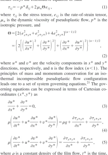
The linear neutral stability curve can be obtained by set- ting d

_i

⫽0 for Eq. 共47兲. Figure 2 shows the linear neutral stability curves of pseudoplastic film flow with different val- ues on flow index n. The results indicate that the linearly unstable region (d

_i

⬎0) becomes larger for a decreasing n.

The temporal film growth rate is computed by using Eq.

TABLE I. Various states of the Landau equation.

Linearly stable

共subcritical region兲

di

⬍0

Subcritical instability E1

⬍0

Subcritical

共absolute兲

stability E1

⬎0

␧a

0

⬍ 冉

^Ed1i

冊

^1/2

␧a

0

⬎ 冉

^Edi1

冊

^1/2

a0→0

a0→0

a0↑

Conditional stability

Subcritical explosive state

Linearly unstable

共supercritical region兲

di

⬎0

Supercritical explosive state E1

⬍0

Supercritical stability E1

⬎0

a0↑

␧a

0→

冉

^Ed1i

冊

^1/2

Nc_r→dr

⫹d

i

F1

E1

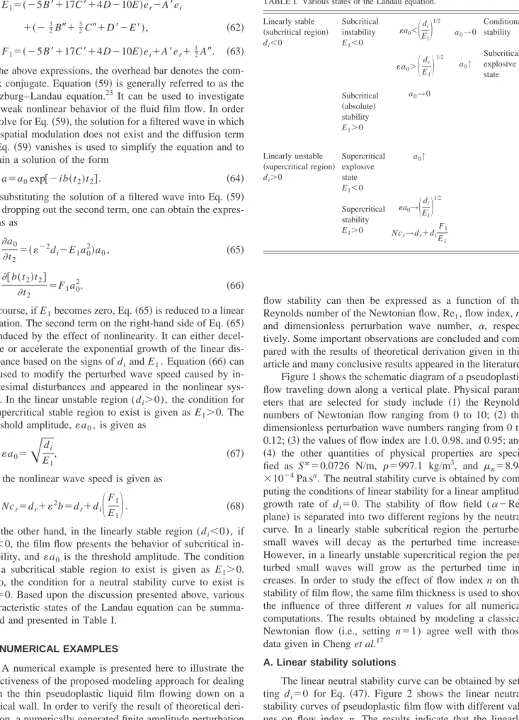
共47兲. Figures 3共a兲 and 3共b兲 show the temporal film growth rate of pseudoplastic fluid for n ⫽0.98 and n⫽0.95 as com- pared to that of Newtonian flow 共i.e., n⫽1). It is interesting to note that temporal film growth rate decreases for an in- creasing n and a decreasing Re

₁

. Furthermore, it is found that both the wave number of neutral mode and the maxi- mum temporal film growth rate increase as the value of n decreases. In other words, the larger the value of flow index n is, the higher the stability of a liquid film should be.

B. Nonlinear stability solutions

As the perturbed wave grows to finite amplitude, the linear stability theory is no longer valid for accurate predic- tion of flow behavior. The theory of nonlinear stability should be used to study whether the disturbed wave ampli- tude in the linear stable region will become stable or un- stable. The study also includes the subsequent nonlinear evo- lution of disturbance in the linear unstable region and will develop to a new equilibrium state with a finite amplitude 共supercritical stability兲 or develop to an unstable situation.

As previously discussed, a negative value of E

₁

can cause the system to become unstable. Such a condition in the linear region is referred to as the subcritical instability. In other words, if the amplitude of disturbances is greater than the threshold amplitude, the amplitude of disturbed wave will increase. This is contradictory to the result predicted by us- ing a linear theory. As a matter of fact such a condition in the subcritical unstable region can in some cases cause the sys- tem to become explosive.

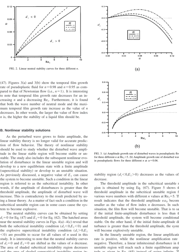
The neutral stability curves can be obtained by setting d

_i

⫽0 for Eq. 共47兲 and E

1

⫽0 for Eq. 共62兲. The hatched areas near the neutral stability curves in Figs. 4 共a兲–4共c兲 reveal that both the subcritical instability condition (d

_i

⬍0,E

1

⬍0) and the explosive supercritical instability condition (d

_i

⬎0,E

1

⬍0) are possible to occur for all values of n used in this study. It is interesting to note that the neutral stability curves of d

_i

⫽0 and E

1

⫽0 are shifted as the values of n decrease.

The area of shaded subcritical instability region decreases and the area of shaded supercritical instability region in- creases as the values of n decrease. The area of subcritical

stability region (d

_i

⬍0,E

1

⬎0) decreases as the values of n decrease.

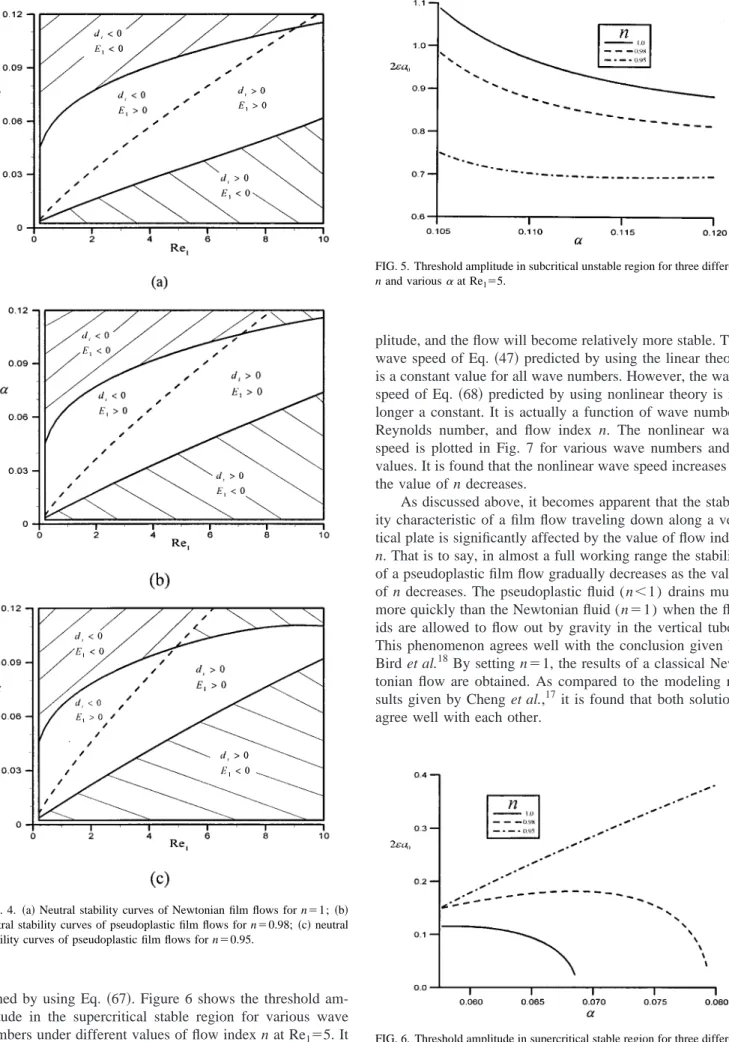
The threshold amplitude in the subcritical unstable re- gion is obtained by using Eq. 共67兲. Figure 5 shows the threshold amplitude in the subcritical unstable region for various wave numbers with different n values at Re

₁

⫽5. The result indicates that the threshold amplitude ␧a

0

becomes smaller as the value of flow index n decreases. In such a situation, the film flow will become unstable. That is to say, if the initial finite-amplitude disturbance is less than the threshold amplitude, the system will become conditionally stable. On the other hand, if the initial finite-amplitude dis- turbance is greater than the threshold amplitude, the system will become explosively unstable.

In the linearly unstable region, the linear amplification rate is positive, while the nonlinear amplification rate is negative. Therefore, a linear infinitesimal disturbance in the unstable region will reach such a finite equilibrium ampli- tude as given in Eq. 共65兲 instead of going infinite. The threshold amplitude in the supercritical stable region is ob-

FIG. 2. Linear neutral stability curves for three different n.

FIG. 3.

共a兲 Amplitude growth rate of disturbed waves in pseudoplastic flows

for three different n at Re1

⫽5. 共b兲 Amplitude growth rate of disturbed waves

in pseudoplastic flows for three different n at␣

⫽0.06.

tained by using Eq. 共67兲. Figure 6 shows the threshold am- plitude in the supercritical stable region for various wave numbers under different values of flow index n at Re

₁

⫽5. It is found that the increase of n will lower the threshold am-

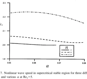
plitude, and the flow will become relatively more stable. The wave speed of Eq. 共47兲 predicted by using the linear theory is a constant value for all wave numbers. However, the wave speed of Eq. 共68兲 predicted by using nonlinear theory is no longer a constant. It is actually a function of wave number, Reynolds number, and flow index n. The nonlinear wave speed is plotted in Fig. 7 for various wave numbers and n values. It is found that the nonlinear wave speed increases as the value of n decreases.

As discussed above, it becomes apparent that the stabil- ity characteristic of a film flow traveling down along a ver- tical plate is significantly affected by the value of flow index n. That is to say, in almost a full working range the stability of a pseudoplastic film flow gradually decreases as the value of n decreases. The pseudoplastic fluid (n ⬍1) drains much more quickly than the Newtonian fluid (n ⫽1) when the flu- ids are allowed to flow out by gravity in the vertical tubes.

This phenomenon agrees well with the conclusion given by Bird et al.

¹⁸

By setting n ⫽1, the results of a classical New- tonian flow are obtained. As compared to the modeling re- sults given by Cheng et al.,

¹⁷

it is found that both solutions agree well with each other.

FIG. 4.

共a兲 Neutral stability curves of Newtonian film flows for n⫽1; 共b兲

neutral stability curves of pseudoplastic film flows for n

⫽0.98; 共c兲 neutral

stability curves of pseudoplastic film flows for n

⫽0.95.

FIG. 5. Threshold amplitude in subcritical unstable region for three different n and various␣^{at Re}1

⫽5.

FIG. 6. Threshold amplitude in supercritical stable region for three different n and various␣at Re1

⫽5.

V. CONCLUDING REMARKS

The stability of a thin pseudoplastic liquid film flowing down on a vertical wall is studied in this article by using the method of long wave perturbation. The generalized nonlinear kinematic equations of the fluid film on free surface of the wall is derived and numerically estimated to investigate the fields of flow stability associated with different n values of flow index. Based on the results of numerical modeling, sev- eral conclusions are given as follows:

共1兲 In the linear stability analysis the neutral stability curve that separates the flow field into two different regions was first computed for a linear amplitude growth rate of d

_i

⫽0. The modeling results indicate the linearly unstable re- gion becomes larger for a decreasing n. It is also noted that the increasing value of n and the decreasing value of Re

₁

will reduce the growth rate of temporal film. In other words, it is interesting to note that the flow becomes relatively stable if it is perturbed by short waves at a low Reynolds number and a larger flow index.

共2兲 In the nonlinear stability analysis, it is noted that the area of shaded subcritical instability region decreases as the value of n decreases. On the other hand, the area of shaded supercritical instability region increases as the value of n decreases. It is also shown that the area of subcritical stabil- ity region decreases as the value of n decreases. It is noted that the threshold amplitude ␧a

0

in the subcritical instability region decreases as the value of flow index n decreases. If

the initial finite-amplitude disturbance is greater than the threshold amplitude value, the system will become explo- sively unstable. The increase of the flow index n will de- crease both the threshold amplitude and nonlinear wave speed in the supercritical stability region, therefore, the film flow will become relatively more stable.

共3兲 The stability of the pseudoplastic film flow decreases as the value of n decreases. When a pseudoplastic liquid film flow is modeled as a non-Newtonian flow, it possesses the characteristic of shear thinning effect. The smaller flow in- dex n of the pseudoplastic fluid will tend to destabilize the flow in motion. Physically, the pseudoplastic fluid of thin film flow will decrease the effective viscosity as the flow travels down along a vertical plane, it can, therefore, increase the convective motion of flow. The decreasing flow index n indeed plays a significant role in destabilizing the flow and is thus of great practical importance.

ACKNOWLEDGMENT

The financial support for this work from the National Science Council of Taiwan through Grant No. NSC 88-2212- E-006-039 is gratefully acknowledged.

1C. S. Yih, Proceedings of the Second U.S. National Congress of Applied Mechanics, New York, 1955, p. 623.

2L. D. Landau, C. R. Acad. Sci. URSS 44, 311

共1944兲.

3J. T. Stuart, J. Aerosol Sci. 23, 86

共1956兲.

4T. B. Benjamin, J. Fluid Mech. 2, 554

共1957兲.

5C. S. Yih, Phys. Fluids 6, 321

共1963兲.

6D. J. Benney, J. Math. Phys. 45, 150

共1966兲.

7S. P. Lin, J. Fluid Mech. 63, 417

共1974兲.

8C. Nakaya, J. Phys. Soc. Jpn. 36, 921

共1974兲.

9M. V. G. Krishna and S. P. Lin, Phys. Fluids 20, 1039

共1977兲.

10A. Pumir, P. Manneville, and Y. Pomeau, J. Fluid Mech. 135, 27

共1983兲.

11C. C. Hwang and C. I. Weng, Int. J. Multiphase Flow 13, 803

共1987兲.

12H. C. Chang, Annu. Rev. Fluid Mech. 26, 103

共1994兲.

13Y. Renardy and S. M. Sun, Phys. Fluids 6, 3235

共1994兲.

14J. S. Tsai, C. I. Hung, and C. K. Chen, Acta Mech. 118, 197

共1996兲.

15C. I. Hung, J. S. Tsai, and C. K. Chen, ASME J. Fluids Eng. 118, 498

共1996兲.

16A. S. Gupta, J. Fluid Mech. 28, 17

共1967兲.

17P. J. Cheng, H. Y. Lai, and C. K. Chen, J. Phys. D 33, 1674

共2000兲.

18R. B. Bird, R. C. Armstrong, and O. Hassager, Dynamics of Polymeric Liquids-Fluid Mechanics

共Wiley, New York, 1977兲, p. 90.

19C. O. Ng and C. C. Mei, J. Fluid Mech. 263, 151

共1994兲.

20C. C. Hwang, J. L. Chen, J. S. Wang, and J. S. Lin, J. Phys. D 27, 2297

共1994兲.

21U. Tomita, Rheology

共Corona, Tokyo, Japan, 1964兲, p. 252 共in Japanese兲.

22D. A. Edwards, H. Brenner, and D. T. Wasan, Interfacial Transport Pro- cesses and Rheology

共Butterworth-Heinemann, Boston, 1991兲.

23V. L. Ginzburg and L. D. Landau, J. Exp. Theor. Phys. 20, 1064

共1950兲.

FIG. 7. Nonlinear wave speed in supercritical stable region for three differ- ent n and various␣at Re1

⫽5.