行政院國家科學委員會專題研究計畫 成果報告
大地工程系統動態可靠度之研究 研究成果報告(精簡版)
計 畫 類 別 : 個別型
計 畫 編 號 : NSC 95-2221-E-011-057-
執 行 期 間 : 95 年 08 月 01 日至 96 年 07 月 31 日 執 行 單 位 : 國立臺灣科技大學營建工程系
計 畫 主 持 人 : 卿建業
計畫參與人員: 博士班研究生-兼任助理:謝宜宏、陳奕竹 碩士班研究生-兼任助理:張景復、陳宏彬
報 告 附 件 : 出席國際會議研究心得報告及發表論文
處 理 方 式 : 本計畫可公開查詢
中 華 民 國 96 年 10 月 03 日
Approximate Real-time Reliability Estimation of Nonlinear Dynamical Systems
with Monitoring Data
Jianye Ching1
ABSTRACT
Updating reliability for nonlinear dynamical systems with high dimensional uncertainties based on monitoring data is a daunting task. A usual way of handling this is to first update the probability density function (PDF) of all uncertainties and then to update the system reliability based on the updated PDF. However, when uncertainties are high dimensional, e.g.: uncertain dynamical excitation, this is not feasible since updating high dimensional PDF is intractable unless the system is linear and all uncertainties are Gaussian.
For nonlinear dynamical systems, this research proposes a way of bypassing the updating step for the PDF of the uncertain variables but directly updating the reliability. Since the updating of the high dimensional PDF is bypassed, the resulting method is feasible for updating reliability of nonlinear dynamical systems with high dimensional uncertainties. Several examples are used to demonstrate and to verify the proposed approach.
Key words: Bayesian analysis, reliability update, monitoring, Subset Simulation
1 (Corresponding Author) Assistant Professor, Dept of Construction Engineering, National Taiwan University of Science and Technology, Taipei, Taiwan. Phone: 886-2-27301055. Email: [email protected].
1. INTRODUCTION
Sensor techniques have been prospering in the recent decade. Many engineering systems, e.g. bridges, buildings, airplanes, etc., are instrumented nowadays for damage detection and health monitoring. An important question is how to update the reliability of these systems based on the monitoring data. However, this is, in general, a very challenging research topic.
An attempt was made by Beck and Au [10] who proposed adaptive Metropolis-Hastings algorithm to first update the probability density function (PDF) of the uncertain system parameters and then to update reliability. A limitation of this approach is that the dimension of uncertainties cannot be too high since updating high dimensional PDF is infeasible. Ching and Beck [11] proposed another method based on ISEE [12] to update reliability of linear dynamical systems. Their approach is not constrained in the uncertainty dimension, but it can be only applied to deterministic linear dynamical systems with Gaussian uncertainties.
Updating reliability of nonlinear dynamical systems remains a pending research problem.
In this research, it is shown that it is not necessary to first update the PDF of uncertain parameters before the reliability is updated when the data is a scalar, i.e. the system reliability can be directly updated. Since the updating of the PDF of uncertain parameters is bypassed, the approach is not limited to the number of uncertainties. To relax the constraint of scalar data, an approximate technique is further proposed to condense all information provided in
the monitoring data into a single scalar data. This scalar data plays a role similar to sufficient statistics, i.e. conditioning on the scalar data, it is assumed that the failure event is approximately independent of the monitoring data.
With the new approach, as long as the PDF of the uncertainties and the probabilistic model of the target dynamical system are given, the approximate functional relationship between the updated failure probability and the scalar data can be obtained prior to the monitoring process. This means in real applications, it is not necessary to conduct the new method in an online manner. Instead, the relationship can be calculated a priori so that the reliability update can be achieved right away once the monitoring data is obtained. It is expected that the new approach is useful for safety monitoring and maintenance of existing engineering systems.
The structure of the paper is as follows: In Section 2, the problem of updating reliability is formally defined. In Section 3, a simple procedure for reliability updating via Monte Carlo simulation (MCS) is presented, while a more efficient method based on SubSim is presented in Section 4. In Section 5, examples are used to demonstrate the new approach, and in Section 6, discussions and conclusion will be given.
2. PROBLEM DEFINITION
The goal of regular dynamical reliability analyses is to estimate failure probability given
the probability distribution of the uncertainties in the target dynamical system and the
probabilistic model
M
of the system, i.e. to computeP F M , where
| F
is the failure event. When monitoring data D is available, it is essential to incorporate it to update the reliability to reduce the uncertainties in the system. This is especially the case if D is the direct measurement on the target dynamical system: this measurement directly reflects the system status. Therefore, it is desirable to develop a methodology to update reliability basedon these measurements, i.e. to compute
P F D M . A usual way of estimating this
| , probability is through the following equation:
( )
1
| , | , | , 1 | ,
N
i i
P F D M P F M f D M d P F M
N
(1)where
contains uncertain parameters of interest, and is drawn from
( )if
|D M
, .Here it has been assumed that conditioning on
, D and the failure event are independent.
With this approach, the PDF of the uncertain parameters is first updated through stochastic simulation, and then the updated reliability is simply the average of the reliabilities for which the uncertain parameters are fixed at their sampled values.
This approach of updating reliability is feasible when the
dimension is low. Beck
and Au (2002) has demonstrated that this approach works reasonably well when the dimension is less than five. When the dimension is high, e.g.: thousands, this approach
may be problematic since drawing samples from the high dimensional PDFf
|D M
, istechnically challenging, and in many instances, practically infeasible. To circumvent this
difficulty, in Beck and Au (2002),
only contains uncertain structural parameters, while the
uncertain excitation is assumed to be stationary Gaussian so thatP F |
( )i, M
can becomputed analytically based on the out-crossing rate method (Soong and Grigoriu 1993). The stationarity assumption may be reasonable for winds and ambient vibration, but not for strong motions and impacts, e.g.: earthquakes, which are obviously non-stationary by their nature. In order to remove the stationarity assumption, it seems necessary to augment the uncertain strong motions into
, but this, unfortunately, leads back to a high dimensional problem.
An exception occurs when the target dynamical system is linear and all uncertainties are
jointly Gaussian. In this case, it can be shown that drawing samples from
f
|D M
, iseasy since it is jointly Gaussian (Ching and Beck 2007). However, for nonlinear systems, the Gaussianity does not hold.
In this paper, a new approach of approximate reliability updating that is applicable to nonlinear dynamical systems with high dimensional uncertainties is proposed. The basic idea of the new approach is described as follows: If the monitoring data D can be transformed into a scalar index
( ) D
such that conditioning on ( ) D
, D and the failure event are approximately independent, i.e. ( ) D
is an approximate sufficient statistics of D from theperspective of the failure event, it is argued that
| , | ( ), , | ( ),
P F D M
P F D D M
P F D M
(2)where for the first equality, we have used the fact that conditioning on D,
( ) D
does notprovide extra information with respect to D. According to Bayes’rule
( ) | , |
| ( ),
( ) |
( ) | , |
( ) | , | ( ) | C, 1 |
f D F M P F M
P F D M
f D M
f D F M P F M
f D F M P F M f D F M P F M
(3)
where
F
C denotes the non-failure event. Note that in this approach, the updating of the PDF of the uncertain parameters is not involved, i.e. it is bypassed. Therefore, the dimension
of does not impose any limitation on the approach.
This new approach thus requires two components: (a) the search of such an approximate sufficient statistics
( ) D
, and (b) the determination ofP F
| ( ), D M
, the failure probability given the scalar data ( ) D
, which, in turns, requires the knowledge of( ) | ,
f D F M
,f ( ) | D F
C, M
, andP F M . In the next two sections, the detailed
| descriptions for estimatingf
( ) |D F M
, ,f ( ) | D F
C, M
, andP F M
| by usingMonte Carlo simulation (MCS) and Subset Simulation (SubSim) will be given. In a later section, a way of finding the approximate sufficient statistics
( ) D
for dynamical systemswill be proposed.
For notational simplicity, the symbol
M
in the conditions will be dropped and will
denote ( ) D
in all the following discussions. Readers should keep in mind that all results are always conditioned on the assumed probabilistic modelM
.3. ESTIMATION OF P F
| VIA MCS
An approach of estimating
P F
| based on MCS is presented in this section. This
approach is inefficient whenP F
| is small. However, the MCS approach is worth
mentioning because of its simplicity. A more technically involving technique that is efficient for smallP F
| based on SubSim will be presented in the next section.
Let
R ( ) denotes the limit-state function that defines failure event F
, i.e. failure event is defined asR ( ) 1
. The MCS method of updating failure probability is described as follows: First, drawN
sets of samples
( )i: i 1... N
from the prescribed PDF of,
each sample corresponds to a monitoring data sample
D
( )i , and hence a sample of( ) ( )
( )
i i
D
, and a limit-state valueR
( )i R
(
( )i ). Throughout the paper,
( )i: i 1... N
will be denoted by
(1: )N for notational convenience, and similar for other variables.According to the Law of Large Number, we have
( )
1
1 1 ˆ
N i i
P F I R P F
N
(4)where
I
is the indicator function: it is equal to 1 if the inside statement is true; otherwise, it is 0. Please note that in the process of MCS, samples distributed asf
|F
and |
Cf F
can be obtained (F
C denotes the non-failure event): Assuming that among theN
samples, there areN
F failure samples, i.e. samples satisfyingR
( )i , so the1 corresponding samples are distributed as f
|F
. On the other hand, there areN
N
F non-failure samples, so the corresponding samples are distributed as f | F
C .With these samples, the unknown PDFs
f
|F
andf | F
C can be estimated byusing histograms. Let us denote the estimated histograms by
f
ˆ | F
andf ˆ | F
C . As aconsequence,
ˆ | ˆ
| ˆ | ˆ ˆ |
C1 ˆ
f F P F P F
f F P F f F P F
(5)
The performance of MCS in estimating
P F
| is independent of the number of
degree of freedom of the system, system complexity, and the uncertainty dimension. In spite of this, MCS is inefficient whenP F
| is small. The reason for this inefficiency is
two-fold: (a) MCS is inefficient in estimating smallP F . This is because the
R
samples from MCS, i.e.R
(1: )N , mostly cluster in the main support region of the PDF ofR
, denoted byf r . However, in order to estimate small
P F
accurately,R
samples in the tail are needed. Unfortunately, MCS is inefficient in propagating samples into the tail region; (b) most failure samples drawn fromf
|F
via MCS reside in the main support region of |
f F
. However, in order to estimatef
|F
accurately for the smallf
|F
region, failure samples in the tail of
f
|F
are needed. Again, MCS is inefficient for this purpose.4. ESTIMATION OF P F
| VIA SUBSIM
According to the previous discussion, the main drawback of MCS in estimating
|
P F stems from the fact that it is inefficient in propagating R
and | F
samples into the tail regions off r
andf
|F
. In this section, SubSim is introduced and employedto propagate the samples into the tail in a more efficient manner. The SubSim procedure of propagating
R
and | F
samples is identical. Therefore, we denoteG
be the uncertain quantity of interest to represent eitherR
or | F
to ease general discussions.4.1 Procedure of SubSim
SubSim provides a more efficient way to propagate
G
samples into the tail off g .
The benefit brought by SubSim is that the tail part of
f g
can be estimated more accurately, hence the area under the tail part, i.e.P G
b
(b
is large), can also be estimated more accurately. Note that here we have constrained ourselves in exploring the right tail. The same procedure can be used to explore the left tail if the sign ofG
is reversed.In the following, the procedure of SubSim of estimating the tail part of
f g
and the area under the tail part is explained.The first stage of SubSim is an MCS step: draw
N
samplesG
(1: )N fromf g . Note
that these samples cannot effectively populate the tail of
f g . The next step is to choose a
threshold
b . Suppose there are
1N
1 samples less thanb ; therefore,
1P G
b
1and 1
P G
b
are roughlyN N and
1 1 N N 1 , respectively. These samples, denoted by1 1
(1:N)
G
b , are distributed asf g G
| , while the otherb
1N
N
1 samples greater thanb
1 are distributed asf g G
| . Theseb
1N
N
1 samples are used to generateN
1 more samples that are also distributed asf g G
| b
1by using the Metropolis-Hastings algorithm [12]: simply conduct the Metropolis-Hastings algorithm with the stationary PDFbeing
f g
but enforce the acceptance criterionG
. Together with the originalb
1N
N
1 samples, there are, again,N
samples distributed asf g G
| .b
1Now the next threshold is chosen to be
b . Suppose there are
2N
2 samples less thanb ;
2therefore,
P G
b G
2| b
1andP G
b G
2| b
1are roughlyN
2N and
1 N 2N
, respectively. TheseN
2 samples, denoted by 21 2
(1: ) ,
N
G
b b , are distributed asf g b
| 1 ,G b
2while the other
N
N
2 samples greater thanb are distributed as
2f g G
| . Thenb
2these
N
N
2 samples are used to generateN
2 more samples so that there are, again,N
samples distributed as
f g G
| . The same procedure is repeated until enough samplesb
2have propagated to the desirable tail region of
f g . Later in the examples, the sample
number
N
in the above descriptions will be called the stage sample number since the sample number remains constant and is equal toN
for all stages.For notational simplicity, the following notations will be used throughout the paper:
1
,
1b b
f g P
denote f g G
| b
1 , P G b
1
, , 1, 1|j j j j
b b b b
f
g P
denote
| j j 1
, j 1| j
f g b G b
P G b
G b
,
f
bm g
denotesf g G
| b
m,, 1 j j
P
b b denotes
j j 1
P b G b
, andbm
P
denotesP G
b
m.Suppose the procedure is repeated for
m stages, the following samples will be
available: 11
(1:N)
G
b distributed asf
b1g ,
11
(1: ) ,
j j j
N
G
b b distributed asf
b bj, j1g
(j 1,..., m 1
),and (1: )
m
N
G
b distributed asf
bmg . Also, the following probability estimates are available:
1 1
P
b N N
,1| 1
j j
b b j
P
N
N
(forj 1,..., m 1
). One can see that the tail probability
P G
b
can be estimated as
1 1
1 1
1 1
1
1
1 1 ,
1 1
( ) 1 ( ) 1
,
1 1 1 1
1 1
1 ( )
1 1
( ) 1
| | |
1 1
1
1 1
1
j j m
j
j j
m
m
b j j b b m b
j
N m N j
i i j n
b b b
i j j i n
m N
i j b
i j
i b i
P G b P G b G b P P G b b G b P P G b G b P
N N
I G b N I G b
N N N N N
I G b N
N N
I G b N
1 1
1 1
( ) ( )
,
1 1 1 1 1
1 1
j
j j m
N m N j N m
i n i j
b b b
j i n i j
N N
I G b I G b
N N
(6)
where we have used the fact that
1
1 1 2 1 11
, , , ,
1
1 1
j j j j j j
j
j n
b b b b b b b b b
n
N N
P P P P P
N N
(7)
and that
1 1,2
1,
1
1 1 1 1
m m m
m
j
b b b b b b
n
P P P P N
N
(8)
Moreover,
f g
can be estimated as
1 1 1 1
1 1
1
, ,
1 1 1 1
,
1 1 1
ˆ ˆ 1 ˆ 1
j j j j m m
j j m
m
b b b b b b b b
j
j m
m
j n j
b b b b
j n j
f g f g P f g P f g P
N N N
f g N f g f g
N N N N
(9)
where
f ˆ
denotes the estimated PDF with histograms, e.g.ˆ
, 1j j
f
b bg
is estimated based on the samples 11
(1: ) ,
j j j
N
G
b b by using histograms. Since many samples propagate to the tail region of
f g , the estimated f g
is accurate in the tail.In SubSim, a popular choice is to pick the threshold values
b
j: j 1,..., m
such thatall
P
bj1|bj are roughly 0.9, or equivalently, to takeN
1 N
2 ...N
m 0.9N
. This can be easily done by adaptively choosingb
j as the 90% percentile among1
(1: ) ,
j
j j
N b b
G
. Moreover, thenumber of stages, i.e.
m , is usually chosen such that b
m andb P G
b G
| b
m .0.1 Under this choice, (6) and (9) become
( )
1
10
m N i m iP G b I G b
N
(10)and
1 1 , 1
1
9 ˆ 9 ˆ 10 ˆ 10
10 10 j j m
m
j m
b b b b
j
f g f g f g f g
(11)Since the SubSim samples propagate to the tail in a very efficient way, the
P G
b
estimator is more stable, and the estimated
f g
is much more accurate in the tail region.The performance of SubSim is also independent of the degree of freedom of the system, system complexity, and the uncertainty dimension.
4.2 Estimating P F
| via SubSim
4.2.1 Estimation of P F
and f | F
Cwith SubSim
In the perspective of SubSim,
P F
can be effectively estimated with (10) by takingG
to beR
andb
to be 1 since the failure eventF
is defined asR 1
. To facilitate the discussion of the estimation forf | F
C , let us denote the samples obtained in the j-th
SubSim stage by 11
(1: ) ,
j j j
N
b b , i.e. the samples satisfying b
j R b
j1. The following samples will be available at the end of SubSim: 11
(1:N)
b distributed asf
b1 ,
11
(1: ) ,
j j j
N
b bdistributed as
f
b bj, j1
(forj 1,..., m 1
), and (1: )m
N
b distributed asf
bm . Among
(1: )
m
N
b , there are ,1bm
N
samples, denoted by (1:,1bm,1)m
N
b , satisfyingb
m ; they areR
1 distributed asf
bm,1 . The other samples, denoted by
F(1:N Nbm,1), satisfyR 1
; they aredistributed as
f
|F
. Also, the following probability estimates are available:1 1
P
b N N
,1| 1
j j
b b j
P N N
(for
j 1,..., m 1
), and | 1 ,1m bm
P F R
b
N N
. If the 0.9 rule isadopted, one can verify that
1 1 1 1
1 1
1
, , ,1 ,1
1 1
,1
, ,1
1
|
9 ˆ 9 ˆ 10 ˆ 10
10 10
j j j j m m
m
j j m
m C
b b b b b b b b
j m
j m b
b b b b
j
f F f P f P f P
f f f N
N
(12)where
f ˆ
denotes the estimated PDF based on the samples with histograms.
4.2.1 Estimation of f
|F
In principle, one can estimate
f
|F
based on the failure samples obtained during the last stage of SubSim, i.e.
F(1:N Nbm,1), since these samples are distributed asf
|F
.However, these samples mostly cluster around the main support region of
f
|F
. Asdiscussed as above,
| F
samples at the tail are needed in order to estimatef
|F
accurately at the tail region. This can be achieved with another round of SubSim, described as follows.
Firstly, the ,1
bm
N N
samples
F(1:N Nbm,1) are used to generate ,1bm
N
more samples thatare also distributed as
f
|F
by using the Metropolis-Hastings algorithm. Together with the original
F(1:N Nbm,1) samples, there areN
samples, denoted by
F(1: )N , that are distributed asf
|F
. The purpose of this first step is not to propagate the samples to the tail off
|F
but just to restore the sample number back toN
.Secondly, the SubSim procedure is implemented to propagate the
| F
samples to thetail of
f
|F
: Choose a thresholdb so that there are
1N
1 | F
samples less thanb ;
1 therefore,P
b F
1| andP
b F
1| are roughlyN N and
1 1 N N 1 , respectively.These
N samples, denoted by
1 11
(1: )
| N
b F , are distributed asf
| b F
1, f
b1
|F
, while the otherN
N
1 samples greater thanb
1 are distributed asf
|b F
1, . TheseN
N
1 samples are used to generateN
1 more samples that are also distributed as1 |
f
b F
by using the Metropolis-Hastings algorithm: simply conduct the Metropolis-Hastings algorithm but enforce the acceptance criterionR 1
and . b
1Together with the original
N
N
1 samples, there are, again,N
samples distributed as| 1,
f b F
.Then the next threshold
b is chosen. There are
2N
2 samples, denoted by 21 2
(1: ) , |
N b b F
, lessthan
b , so they are distributed as
2f
|b
1 b F
2, f
b b1,2
|F
. The same procedure is repeatedm times. Finally, the following samples will be obtained:
11
(1: )
| N
b F distributed as1 |
f
b F
, 11
(1: ) , |
j j j
N b b F
distributed as , 1 |j j
f
b b F
(forj 1,..., m 1
), and (1: )|m
N
b F distributed asf
bm
|F
f
| b F
m, . Also,P
b F1| P
b F
1| N N
1 and
1| , 1
| ,
1j j
b b F j j j
P
P b
b F N
N
(forj 1,..., m 1
). If the 0.9 rule is adopted, |
f F
can be estimated as follows: 1 1 , 1
1
9 ˆ 9 ˆ ˆ
| | | 10 | 10
10 10 j j m
m
j m
b b b b
j
f F f F
f
F
f F
(13)where
f ˆ
denotes the estimated PDF with histograms, e.g.ˆ
, 1 |
j j
f
b b F
is estimated based on the 11
(1: ) , |
j j j
N b b F
samples by using histograms.In summary, with two rounds of SubSim,
P F ,
f
|F
, andf | F
C can beeffectively estimated. Together with (5),
P F
| estimate can be obtained. Please note that
SubSim is applicable to general linear or nonlinear dynamical systems whose uncertainty dimension can be arbitrarily large.Besides, with the proposed approach, the functional relationship between the updated failure probability and the scalar data
can be obtained prior to the monitoring process as
long as the probability distribution of the uncertainties and the probabilistic model of the system are given. This means in real applications, it is not necessary to conduct the new method in an online manner. Instead, the relationship can be calculated a priori so that the reliability update can be achieved right after the monitoring data is obtained.5. SELECTION OF SUFFICIENT STATISTICS
6. EXAMPLES
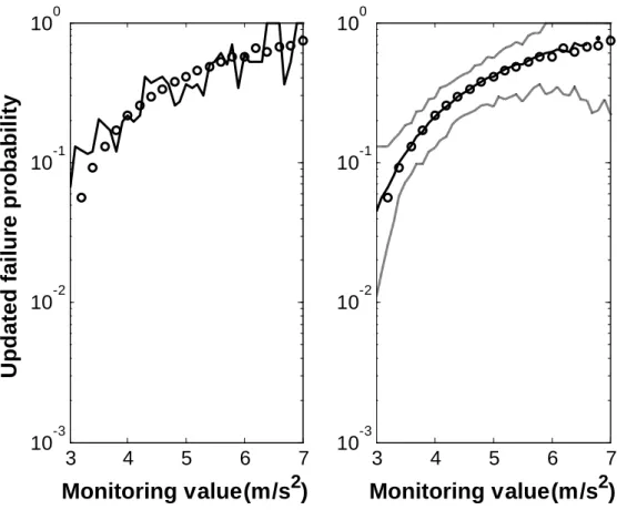
Three examples are selected to demonstrate the use of the new method. The first example is an infinite slope, where the monitoring value is the height of the water table, and the failure is defined as the sliding of the slope. The second example is a ten-story building subjected earthquake motions, where the monitoring value is the maximum acceleration on
the roof, and the failure is defined as the exceedance of the maximum inter-story drift over a prescribed threshold. The third example is a real case study, a deep excavation problem, where the monitoring value is the maximum diaphragm wall deformation, and the failure is defined as the exceedance of the maximum ground settlement over a prescribed threshold.
There are some common features for the three examples: (a) the uncertainties are so significant that the failure probability is quite large when no monitoring data is available; (b) the physical quantities that directly define failure cannot be monitored easily, but the monitored value contains certain information about those quantities, so the knowledge of the monitoring value is helpful in reducing the uncertainties associated with the defined failure.
6.1 Infinite slope
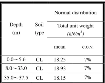
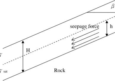
In this hypothetical example, let us consider the infinite slope in Figure 2, where
H
is the thickness of the soil layer, is the slope angle, h
is the height of the water table,
is the unit weight of the soil, and is unit weight of the saturated soil. The failure event is
sat defined as the sliding of the slope along the soil-rock interface, i.e. downward sliding force is greater than the shear resistance along the interface. Therefore, the limit-state function is
2
sin cos cos tan
sat
sat
h H h
R Z h H h
(14)The height of the water table is uncertain and is uniformly distributed over the [0,
H
] interval, i.e.h H U
, whereU
is uniformly distributed over the [0,1] interval. For this example,Z
contains all uncertainties, including
, sat,H
, , . It is assumed that the uncertain U
variables
, sat,H
, are Gaussian with mean equal to 17 kN m /
3,10 ,19 m kN m /
3, 35
and standard deviation equal to 1.5 kN m /
3, 3 ,1.5 m kN m /
3, 3
. The slope angle is
known and is equal to20
. The monitoring value is the height of the water table h
.For this case study, the prior failure probability, i.e. the failure probability without data
P F , is roughly 50%, indicating that the uncertainties are significant. Therefore, it is
desirable to update the failure probability with the monitoring data so that the uncertainties
can be reduced. Both MCS and SubSim are employed to estimate
P F
| , but only the
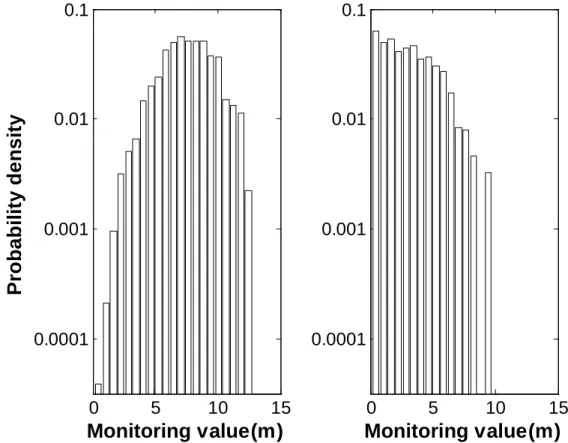
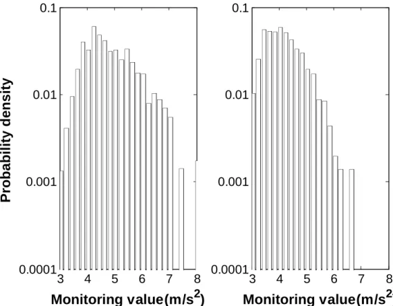
SubSim results will be presented in details while the MCS results are only used for comparison. During SubSim,f
|F
andf | F
C are estimated with histograms, shown in Figure 3. With 錯誤! 找不到參照來源。, the estimate forP F
| is obtained.
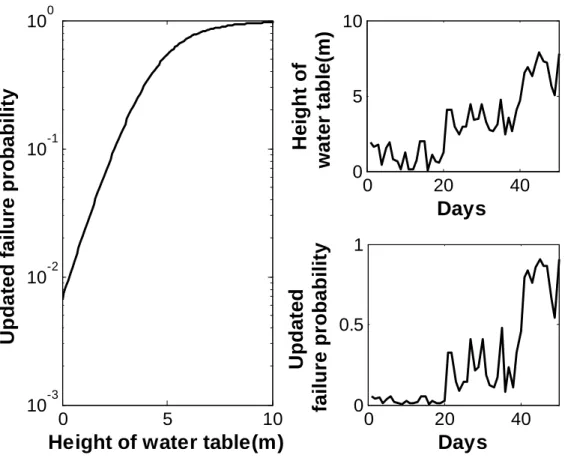
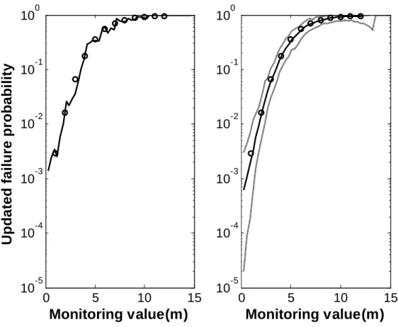
The left-hand-side plot in Figure 4 shows the analysis result of the proposed approach with a single SubSim run with stage sample number
N
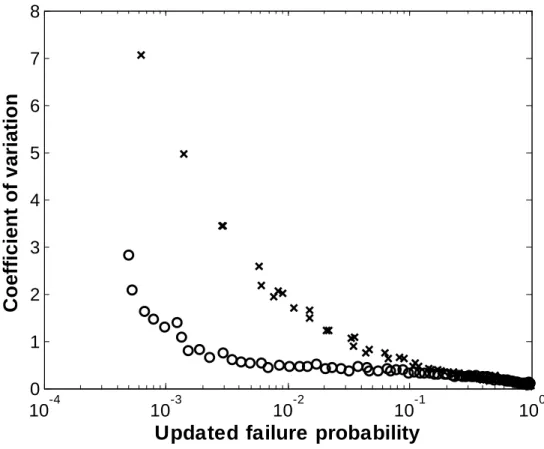
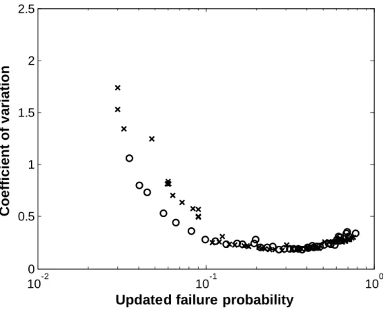
= 1000, which shows that the updated failure probability increases with increasing height of water table. The right-hand-side plot shows the average and 95% confidence interval of the results from independent 200 SubSimruns. Figure 5 shows the comparison of the variabilities in the
P F
| estimates made by
MCS and SubSim with the same total sample number. It is clear that the SubSim approach outperforms MCS due to the fact that SubSim is more efficient in propagating samples into the desirable tail region.To examine the analysis results, let us consider the following verifying procedure:
![Figure 9. An illustration of the deep excavation case study (after Ou et al. [20]).](https://thumb-ap.123doks.com/thumbv2/9libinfo/9127401.411591/40.892.281.615.106.502/figure-illustration-deep-excavation-case-study-ou-et.webp)
