Explaining the Implied Volatility Skew from the Rational Speculation Perspective: Calibration on the Taiwan Stock Index Option Market

Explaining the Implied Volatility Skew from the Rational Speculation Perspective: Calibration on the Taiwan Stock Index

Option Market

Chen, Son-Nan Tsai, Hui-Huang National Chengchi University

National Taipei University

Abstract

Two cornerstones in Behavioral Finance, the limits of arbitrage and investor psychology, can explain the formation of implied volatility skew existing in Taiwan stock index option (TXO) market well.

Adopting the real-time data which exhibits the limits of arbitrage in the futures market and designing two speculation models which describe the trading behavior of the market maker in the option market, this study successfully calibrates out the market maker’s perceived volatility with a view to exhibit the similar pattern to the volatility asymmetry in spot market. The trading behavior of the market maker in the prevalence of positive feedback traders is based upon the argument of Destabilizing Rational Speculation of (De Long et al., 1990) that is well suitable to a market full of noise traders like the TXO market. one thing deserves to mention is that the calibration of our second speculation model, Shifted Speculation Model, on the implied volatility curve involving merely single volatility parameter shows that it is a self- consistent model, improving the often unjustly maligned defect of Black-Scholes Model and conforming to the market practice.

Keywords: Volatility Skew; Rational Speculation; Market Maker;

Stock Index Option; Option Pricing;

1 Introduction

The tremendous success of (Black and Scholes, 1973) and (Merton,1973) is based on the no-arbitrage theory and the true engineering, so-called the dynamic hedging argument, to determines option prices which are irrelevant to investor demand. However, many empirical studies document the existence of well- known option-pricing puzzles – the expensiveness and the skew pattern of stock index options. These puzzles show that BSM can’t be self-consistent. The related literature is surveyed by (Bates, 2003) and concludes that demand- pressure can really affect option prices and that a new pricing approach by market makers is needed.

This paper takes this challenge and tries to explain the above empirical patterns of index option prices from the industry organization in the market:

hedgers, market makers and speculators. (Bollen and Whaley, 2004) asserts that the volatility skew is due to the demand of the put for hedging on the index under the inevitable reality of limits of arbitrage

. The demand for hedging also affects the index futures prices, as (Chen, Cuny and Haugen, 1995) describes.

However, the demand of options seems not to increase monotonically as the moneyness decreases, and then this argument can’t explain the second puzzle properly. Further, whereas financial theory and empirical evidence suggest that derivatives markets exist to facilitate hedging, a more popular perception is that they serve as an instrument of speculation, and the demand for speculation also tend to be invited as the spot volatility increases. Although (Chatrath et al., 2002) describes that the dominance of commercial trading is typical for stock index futures markets, the industry organization in Taiwan market is totally different. The ratio of trade volume made by individual investors is over 70%. It is difficult to believe that the demand for hedging is large enough persistently to affect the option price because that the portfolio tilts of the individuals are more severe than that of the mutual fund managers. In addition there are no designated dealers or specialists in Taiwan markets. It therefore seems quite unreasonable to attribute the volatility skew of Taiwan stock index option (hereafter TXO) market to the demand of options for hedging without any hesitation. In the light of the above observation, this paper is motivated to study the volatility skew in TXO market from the viewpoint of speculation.

The destabilizing rational speculation argument by (De Long et al., 1990) is suited to describe the operation of TXO market. Basically individual investors

1 Capital constraint and agency problems (Shleifer and Vishny, 1997) or collateral requirement (Liu and Longstaff, 2004) can limit intermediaries such as market makers to hedge their positions perfectly.

are commonly seen as the noise traders or irrational speculators; proprietary traders and foreign institutional investors are seen as de facto market makers.

Arbitrage positions undertaken by rational speculators cannot be unlimited because of risk aversion, so noise traders can affect spot prices.

Some kind of noise traders like positive feedback traders – buy when prices rise and sell when prices fall – behaviors on extrapolative expectation,

e.g. extrapolating price changes. They successfully show that how the early trading made by rational speculators’ triggers positive-feedback trading, and then increase volatility about fundamentals. Their view of destabilizing rational speculation is motivated partly by George Soros’ own investment strategy – betting not on fundamentals, but on future crowd behavior. More interest is that this argument can account for the front-running by investment banks. To the best of our knowledge, this argument has yet applied to the stock index option market, not to mention the interactions between the stock market and its derivative markets. This is just the challenge which this paper tries to take on with the help of Behavioral Finance.

As to the implementation of speculation, a complex pricing model is never a top priority. One claim, announced by (Derman and Wilmott, 2009), that BSM is already the consensus pricing model is because of its clearness and robustness. The clearness comes from a true engineering, i.e. dynamic hedge, and then shows the relationship between the implied volatility and future spot volatility under a friction-free market. The robustness means that it allows market players easily manipulate the only input, i.e. volatility, so as to arrive at the price deemed more appropriate by them. The second feature implies that BSM is useful for measuring the relative values among options and that the implied volatility contains the trader’s view on the future in real world, whilst the first one implies that implied volatility may be not equal to the future spot volatility because of the transaction cost, but the innovations of these two kinds of volatilities should be the same or have similar patterns. (Korn and Wilmott, 1988), (“KW” for short) based on the same true engineering as BSM but releasing the requirement of dynamic hedge, provides a framework for hedging and speculating with options to show how the speculator evaluates an option.

One thing that deserves notice is that BSM is a special case in this framework.

2 According to studies related on Taiwan option market like (Barber et al., 2006) and (Chang et al., 2009), only proprietary traders and foreign institutional investors earn money in the Taiwan option market.

Individuals in total lose money.

3 Extrapolative expectation is verified with the experiment in (Andreassen and Kraus, 1988). Subjects with some training in economics and shown with authentic stock price patterns will reveal this phenomenon.

4 (Shleifer and Summers, 1990) has a similar but more detailed discussion on the so-called “the noise trader approach to Finance” from the arguments of both the “limits of arbitrage” and the “investor sentiment”. And these two arguments are exactly the two cornerstones of Behavioral Finance.

This paper adopts the analysis of (De Long et al., 1990) and follows KW to design pricing models for measuring subject values of TXOs to rational speculators. Rational speculators in this paper are assumed to be market makers who utilize the directional information from the stock index futures and then determine their prospecting volatility of the stock index by referring some patterns in stock market. This is similar to bet on the future crowd behavior in De Long et al. The most possible pattern relating both direction and volatility of the stock market is the volatility asymmetry. We call the implied volatility calibrated from models about speculation the perceived volatility with a view for convenience. In opposite, the implied volatility from BSM, without directional information in it, should reflect the level of demand on option from noise traders. With the empirical calibration on the real-time data of TXO, the first finding in this paper is that while implied volatility from BSM violates the internal arbitrage,

the perceived volatility with a view does not. Then this paper finds that the perceived volatility with a view can fit the skewed volatility curve well. This means that the perceived volatility with a view designed by us can measure the unique future spot volatility prospected by market makers and that the pricing models in this paper are self-consistent. Finally, from the skewed volatility curve, this paper calibrates out the reverse relation between the speculator’s expected future spot prices and his perceived volatilities of the underlying asset. This verifies our projection that the rational speculator may determine his perceived volatility with a view in option market by referring the volatility asymmetry in spot market. And this is the major contribution on this paper. For one thing it supplements the literature of investigating the whys and wherefores behind the volatility skew of the stock index option market from the supply side of option, for another it supports the literature of studying implied volatility and future portfolio returns, dating back to (Giot, 2005).

The remainder of this article is organized as follows. Section 2 takes the related literature review. Section 3 introduces the models extended by us for describing the behavior of the rational speculator. Section 4 presents and interprets the calibration results with TXO market data and Section 5 draws the conclusion and suggestion.

2 Literature Review

One strand of empirical options research seems substantially focused on

5 Free of internal arbitrage means that by put-call parity the volatility of put should be the same as that of call. The arbitrage in BSM is volatility arbitrage, i.e. deviation of the implied volatility and the future spot volatility. However, the future spot volatility is uncertain at the time of trade.

stock index options. (Bates, 2003) divided it roughly into testing on BSM paradigm and on alternative models. After empirical scrutiny of alternative option pricing models, he concludes that alternative models still leave much room for improvement. In opposite, based on empirical evidence of two puzzles about volatility - volatility bias and volatility skew/smirk from tests of BSM, he suggested that a new pricing approach be consistent with industry organization, i.e. hedger, market maker and speculator, is desirable. As the stock index options markets function as an insurance market for portfolio. The predominant demand from institutional investors can affect the prices of options; whereas competitive market making firms predominantly write them. Small market fluctuations can be delta-hedged by these firms, but jump and volatility risks are perforce unable to be eliminated and only be transferred to another market maker. Thus market makers will limit their exposure to these risks and can not supply option unlimitedly.

As a matter of course options become expensive.

Further, the demand of put is the reason of formation of the volatility skew, also supported by (Bollen and Whaley, 2004). However, when market makers function as intermediates, they can not neglect the impact from speculators. Not to mention that the impact from speculation is more severe in some emerging markets which are predominated with individual investors.

To the best of our knowledge, the option pricing research is rarely related to speculation. (Korn and Wilmott, 1988) constructs a portfolio consisting with an option, some stock and some zero coupon bond – similar to the true engineering in BSM, but the trader can choose either full hedge, partial hedge or pure speculation. The replacement of dynamic hedge requirement with strategy choice allows the trader to evaluate an option with subjective adjustment. So KW provides a framework for hedging and speculating with options and it can be used to show the subjective value or shadow price of an option to the trader.

One thing that deserves notice is that BSM is a special case in this framework.

However, the empirical study related to speculation is still rare because that it is so difficult to estimate the growth rate of the underlying asset and the betting direction of speculation in option market is so violate in reality.

But, at least, the impact of speculation in futures markets on realized spot volatility was discussed widely for a long time. Date back to (Friedman,1953), when the basis

between the spot and futures market is large enough, the rational speculator will arbitrage and buck the trend, then make prices stable and

6 (Shleifer and Vishny 1997) proposed that capital constraints and agency problems will induce the limited supply of options. (Liu and Longstaff 2004) also proposed that collateral requirement has the same result.

7 The basis is defined in this paper as the futures minus the forward price of the spot market index.

alleviate the observed volatility of the underlying asset. In the opposite case, (De Long et al., 1990) believe that if enough traders adopt the positive feedback strategy, the long position by a rational speculator will trigger their action and the futures price will deviate further from the spot price. The future spot price still has the ability to rise above the current futures price. This is just so-called destabilizing rational speculation and coheres with the Normal Backwardation theory proposed in (Keynes, 1930), although this theory discusses commodity, not stock index. Based on its key hypothesis—that the hedger should compensate the speculator for bearing the uncertainty of price—(Kolb and Overdahl, 2006) concludes the following price patterns for futures. When the basis is positive, the estimated future spot price is higher than the futures price.

In the opposite case, when the basis is negative, the estimated future spot price is lower than the futures price. These two situations are called Normal Backwardation and Normal Contango, respectively. Thus, we know how the speculator in the futures market influences the realized volatility of the underlying from the basis, which reveals the market player’s anticipation of the direction of price change.

On the contrary, there is a strand of literature study the impact of spot volatility on the basis. (Chen, Cuny and Haugen, 1995) presents that the basis decreases as the spot volatility of the S&P 500 increases, and vice versa. As spot volatility increases, the open interest in futures increases. This observation is supported by (Chang, Chou and Nelling, 2000) as the Open interest is used as a proxy for hedging demand. However, (Chatrath, et al., 2002) provides a little different result. Futures leadership is undisputed when markets are bull and without feedback from the spot market. In contrast, when markets are falling, futures leadership is not significant but the feedback from the spot market is detected. They also find a positive relationship between basis and spot volatility.

That is different to the conclusion of (Chen et al., 1990), but can be explained by the predisposition of commercial traders to select index trading over trading in stock portfolio when positive information arrives. Examining S&P 500 Stock Index futures, (Pan, Liu and Roth, 2003) find that volatility positively affects demands both for hedging and speculating and the futures risk premium just affects demands for speculating, not hedging. In short, the dynamic relation between spot volatility and basis behavior or futures risk premium depends on the trader selectivity.

However, the more significant the anticipation on the direction of spot

market, the more significant some kind of trader selectivity will be induced, and

then the prices of its derivatives will be influenced. The detailed discussion in

the futures market is well established on the debate between Friedman and Keynes. As to the option market, only the role of arbitrager is involved, e.g.

(Bollen and Whaley, 2004), and the role of market makers and speculators is yet discussed. This paper tries to fill this gap with the destabilizing rational speculation proposed by (De Long et al., 1990). To investigate the behavior of speculators in stock index option market, this paper supposes that speculators in stock index option markets can be divided into rational speculators and irrational speculators (positive feedback traders) and further that rational speculators play the role of market makers and make decision by guessing the future crowd behavior formed by irrational speculators. As market makers, they can not hedge option perfectly and are sensitive to risk because of limited capitalization.

This implies that the supply of options is limited. This paper tries to design models of speculation within the general framework of KW, and then calibrate the implied volatility of them, i.e. perceived volatility with a view, with TXO data. The data will be chosen when the absolute value of the basis is as large as possible to obey the rational speculation argument of (Friedman, 1953). This volatility should have some features similar to spot volatility as we hope. Here are features which we want to get.

(1) The perceived volatilities of a call and of a put at individual strike price should be the same or near.

The rationale behind it is that since market makers have the willing to provide liquidity, the values of a call and a put with a same strike price should not be different to them even when the direction of the stock market is significant. Otherwise the internal arbitrage will appear. Similarly, the volatility curve made of Out-of-money (OTM) options should be smooth; otherwise this means an opportunity of butterfly spread arbitrage. In summary, implied volatility can reflect the market situation, but perceived volatility should not because it reflects the value of an option to market makers.

(2) The perceived volatilities of OTM options across strike prices should be the same.

This is based on the feature of only one single underlying asset. If the volatility curve of OTM options can be fitted well by our models, we at least can say that the model does not violate the assumption of single constant volatility.

(3) The perceived volatility should have a reverse relation with the anticipated spot price in the future.

8 For the detail about market makers’ behavior, see (Bates, 2003).

The rationale for this feature is that rational speculators guess the future crowd behavior. Whatever the future direction of the spot market they project, the volatility of the underlying asset they anticipate should adjust at the same time. This is based on the strategy used by positive feedback traders:

extrapolative expectation. One stylized pattern in stock market is volatility asymmetry: when the market trend is upward, the volatility tends to be small;

when the market trend is downward, the volatility tends to be large. The perceived volatility used by rational speculator to quote for option should has the similar pattern as the spot volatility has.

To summary, the first feature investigates whether the perceived volatility with a view can measure the relative values of options. If the value can be measured correctly, a call or a put should be indifferent to market makers regardless of the significant trend of the spot market. The second feature is to show the consistence of a model in the pricing of options with different moneyness: one underlying asset, one implied volatility. The third feature is based on the view that when the perceived volatility can correctly measure the value of an option to market makers, their decision-making should refer the observed pattern in spot market to provide liquidity.

3 Models

3.1 Naive Speculation Model

With the exception of the arbitrager and the hedger, KW classifies other players in the option market into two types: the pure speculator and the partial- hedging speculator. The pure speculator wants options only for speculation. The partial-hedging speculator may use a partial hedging approach to bound his risk.

The choice of strategy will determine his required rate of return on the portfolio, including a bond, a risk asset (known as a stock index in this paper), and an option. Similarly to BSM, KW framework supposes that the related dynamics of the bond and the stock index under the actual measure,

, are respectively given:

t t

dB rB dt

,

(1)

P

t t t t

dS 





，

(2)

where

is the risk-free rate of the bond,

and ^ and ^ respectively denote the growth rate and the volatility of the underlying asset,

. These three parameters without any subscript

are all assumed constant.

is one- dimensional Brownian motion. The initial values of the bond and the underlying asset are respectively 1 and

.

An investor who holds a European option with a maturity

and a final payoff

also trades in the underlying and the bond to hedge his option fully or partially against the uncertainty from this position. The subjective value of the option at time

when the underlying asset is

,

, could be determined in the following equations.

2 2 2

2

1 0

2

V V V

S yS rV

t  S S

      

   (3a)



  

V T S  f S

(3b)

where

is a constant which is determined by the trader selectivity. If the trader adopts a full hedging strategy, the

in equation (3a) will be equal to

and this equation will be the same as BSM’ PDE; otherwise, the trader will be attributed to a speculator. When the trader adopts a pure speculating strategy,

will equal to ^ . When the trader adopts a partial hedging strategy,

will be located between ^ and

. This paper supposes that the trader adopts a pure speculating strategy in the option market and requires the same compensation for bearing the uncertainty in price as in the futures market, as described in Normal Backwardation Theory. Just as (Hull, 2006) analyzed the risk in the futures positions, we can find that the relationship between the futures price with maturity

at time

, denoted as

, and the estimated future spot price at time

T

, denoted as

, is

( )( )

T P( ) r k T t

t t T

Fu E S e ^{ }

(4)

where

is a discount rate suited to the investment and the absolute value of

k r

is the required rate of return by speculators. Under the actual measure, we know that

. Equation (4) could therefore be rewritten as the following:

( )( ) ( )

T r k T t g T t

t t t

Fu S e^{   } S e ^

(5)

9 For details about this framework, see Appendix A.

where

is a proxy for the basis risk between the futures and the spot markets.

When the absolute value of

is larger, it is usually said that the opportunity of index arbitrage emerges and the trend will be bucked by the rational speculation argument of Friedman. However, it is differently viewed from the Normal Backwardation Theory of Keynes. By (Kolb and Overdahl, 2006) this means that

is approaching ^ and this implies that speculation dominates the futures market. In the opposite case of

approaching

, this implies that hedge dominates the futures market.

It is a conventional wisdom that from the view of speculators the stock index futures is a instrument to bet on the direction of spot market and the stock index option is one to bet both on the direction of spot market and on the average volatility during the life of the option. Market players are not limited to enter the futures or option market. The basis risk in futures of Taiwan Stock Market Index (TX, henceforth) should have provided a hint for investigating TXO market.

It is naturally to replace

in equation (3a) with

to evaluate the subjective value of an option to the speculator. Calibration with market data will enable us to measure the speculator’s perceived volatility with a view on the direction of spot market. Being a de facto market maker in option market who gets some compensation from the futures trading, the rational speculator will treat a call and a put equally without discrimination.

After applying Feymann-Kac Theorem, it is trivial to derive the value of a European call option,

, with a strike price,

:

 

1 2

( , )_t ^{g r T} ( ) ^rT ( )

C t S Se ^ N d Ke^ N d

(6)

where

2

1

ln 1

2

S g T

d K

T





     

   

   

 ,

^

and

is the Cumulative Normal Distribution.

It needs similar effort to derive the value of a European put. In this paper, we call it the “Naive Speculation Model” (NSM) because so far it cannot be applied to implied volatility curve; yet, it does provide a method for measuring the relative values of TXOs, even when the basis risk of the Taiwan stock market index futures, TX is large, at the same time, the difference between the

10 In practice, to hedge the position of an option, the trader uses the TX contract, not the real underlying, i.e.

the stock market index, because of the difficulty to replicate it. Then the (Black, 1976) is used to derive the implied volatility. However, this approach has at least two shortcomings. One is that futures prices do not follow random walk because of the existence of futures risk premium, as (Bessembinder, 1992) suggested; the other is that the spot volatility is not independent to the levels of the basis, as (Chen, Cuny and Haugen, 1995) proposed.

implied volatility of NSM and that of BSM will be significantly revealed. That is just why we call the implied volatility of the speculation model the perceived volatility with a view.

3.2 Shifted Speculation Model

The futures price stands for traders’ “major opinion” about the future spot price at maturity in the futures market. In the option market, the estimation of future spot price at maturity will induce the trader to choose some options with specific strike prices; thus, the major opinion about the future spot price is not necessarily formed in the option market. Since this paper assumes that the speculator makes a decision about perceived volatility by referring to the volatility asymmetry pattern, his estimation on the future spot price will play an important role

. This induces us to modify the dynamics of the underlying asset, in a similar way to (Rubinstein, 1993) and (Marris, 1999), in the following form:

( , ) ^T

t t

dF 



，

(7)

( , ) _t (1 ) 0

A t F 





(8)

where

is the forward price of the stock index and

is the price of a zero coupon bond.

is a Brownian motion under the forward measure.

represents the forecast of the future stock index with maturity

by the speculator at time 0, in other words the future stock index at maturity estimated by the speculator at the current time. When offering a price for an option, the speculator estimates the average volatility in the life of that option, i.e. ^ . The function

describes the future spot price level forecasted by the market, the individual speculator or some kind of combination. No matter what the setting of this function exploits the advantage of BSM – robustness – as (Derman and Wilmott, 2009) describes and it conforms to the market practice:

manipulating the only input – volatility – so as to arrive at the price of an option deemed more appropriate by traders.

This dynamics has some interest features. When ^ is equal to 0, it will yield a Normal absolute diffusion process; when ^ is equal to 1, it will yield a Log-Normal diffusion process, similar to BSM. Whatever happens, in this paper

11 The argument that the implied volatilities are related to their moneyness is not unique in our paper.

(Derman and Kani, 1998) assume that local variance is the risk-neutral expectation of instantaneous variance, conditional on the fact that the stock price at maturity will equal the strike price. This assumption implies that local volatility is determined when the expectation of the future stock price at maturity is equal to the strike price. However, that paper and its followers are based on risk-neutral pricing approach; our paper is different to them from the viewpoint of speculation.

that parameter is used for calibrated from trading data and shows the mixed view of all traders in the option market. Using the Feymann-Kac theorem and variable transformation, it is trivial to derive the pricing formula of European call as follows.





0 0 1 2

(0, )

(0, ) B T ( ) ( )

C f X N d K N d

  

, (9)

where

^

^

and

^

^

0 2

* 1

ln 1 ( )

2

X T

d K

T





 

and

0 2

* 2

ln 1 ( )

2

X T

d K

T





 

.

Similarly, we can get the close-form solution of the put. In this paper, we call the above result “Shifted Speculation Model” (SSM) and use it to calibrate the implied volatility curve in TXO market.

4 Calibration Result

As occurs in other emerging markets, in the Taiwan stock index derivatives market we also confront the problem of liquidity. The majority of trades focus on the near-month contract, so this note focuses on the study of the implied volatility curve, not its surface. To investigate the effectiveness of these two speculation models on the trading of TXO,

this paper uses two samples while the basis risk of the MTX is as large as possible because that it is the chasm among the arguments about rational speculation. In other words, we adopt the subjects located in the limits of arbitrage (strictly speaking, this is an index arbitrage between the stock market index and its futures) and use speculation models to investigate the market maker’s psychology in such unusual situations.

The subjects are the real-time data located in two extreme market situations: An inverted market case with

at 12:40 p.m. on October 30, 2006 and a normal market case with

at 10:10 a.m. on October 24, 2006.

indicates the deviation of TAIEX index and MTX maturing on November 15,

12 TXO market deserves to be studied because of not only its organization full of individual investors, but also its non-neglected scale compared to other emerging markets. According to the survey of the World Federation of Exchanges at 2007, its underlying asset, Taiwan Stock Exchange, has been ranked 21^st in the world in terms of market capitalization, and 17^th in the world of trading volume. In addition, TX and TXO were ranked 14^th and 4^th most frequently traded index derivatives on a global scale. For further detail, please refer (Chang, Hsieh and Wang, 2009).

2006 as in equation (5)

. The risk-free rate is 1.75%, which is a one-month interest rate of CD in the Taiwan Bank. The result will be shown in three steps.

Firstly, we show the performance of NSM and BSM for measuring the relative values of TXOs. Then we calibrated the SSM and compare it with the Stochastic

 model, also called the SABR model,

proposed in (Hagan et al., 2002).

Finally, we show the relationship between the anticipated future spot price and the implied volatility from SSM, i.e. the perceived volatility with a view, and then provide our findings.

4.1 The Measurement of the Relative Values of Options

One of the functions of implied volatility is to measure the relative values of options. We use two criteria to compare the implied volatilities derived from BSM and NSM.

1) The deviation of the implied volatilities between the put and the call at the same strike price should be small. Otherwise, it will be misled to a signal of internal arbitrage.

2) The implied volatility curve made of out-of-the-money (OTM) options should be smooth. Otherwise, it will be misled to a signal of butterfly spread arbitrage.

The rationale behind the criterion 1 is that when the anticipation on the market trend is significant, either the demand of the put or the call will be significant at the same time, depending on the market is going down or up. Then the relative values between the put and the call will reflect on their implied volatilities derived on BSM, because that BSM can measure the value of an option to its end-users, hedgers and/or speculators. In opposite, since NSM is designed to measure the value of an option to (de facto) market makers, we could hope that the perceived volatilities of a put and a call, derived from NSM, should be indifferent because that their function to market makers is just to provide liquidity. As to the rationale of the criterion 2, BSM in practical allows the traders to qualitatively adjust for higher possibility of extreme market movement than in Normal distribution by manipulating the volatility of out-of-

13 The reason of using real time data is that market makers usually take positions before close which are against their earlier view to avoid the risk coming in the next workday. By this reason the data obtained at close is not suited to describe the behavior of market makers.

14 It is a famous model which provides good fits to the implied volatility curves. (West, 2006) uses it to investigate illiquid markets and get good result. However, it needs the Singular Perturbation Approach to get the close-form solution and that is too complicate to be used by market makers. For a little more details about this model, see Appendix B.

money options, so the implied volatility curve should be smooth to market makers. If not, we can project the reason from the view of end-users.

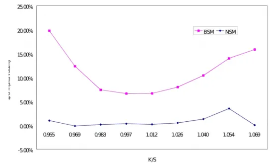
In Figure 1, the result of BSM can be easily explained by the argument of (Bollen and Whaley, 2004): the demand of options will influence their prices.

The Case 1, an inverted market condition, tells us that the future spot price is expected to be lower than the current spot price by (Keynes, 1930) and the demand of the put increases at the same time. This then induces the value of the put to be higher than that of the call with the same strike price. This is why the implied volatility gaps between the put and the call, i.e. the implied volatility of the put minus one of the call, at the same strike price, derived from BSM, are higher than zero. On the contrary, the Case 2, a normal market condition, just tells us that the future spot price is expected to be higher than the current spot price, so naturally the demand of the call increases. It is then easy to see that the implied volatility gaps derived from BSM are lower than zero. This implies that the value of a call is higher than that of a put with respect to strike price at such a market situation. The above cases both mislead to a signal of internal arbitrage; however, from the view of NSM, after including the compensation to price uncertainty in futures trading as Keynes said, the values of the put and the call should be indiscriminative to the rational speculator no matter whether the future spot price will go up or down. Hence, the gaps of implied volatility of the put and the call at the same strike price are near zero, as shown in both cases.

[Insert Figure 1 here]

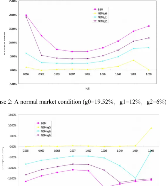
To see the impact of the basis risk on it, we add additional two minor

s in each case: -6% and -3% in case 1 and 12% and 6% in case 2 to implement the sensitivity analysis on the basis. Following the same reasoning as above with the result of Figure 2, we can easily find that using the basis existing in the futures market is the optimal choice for the market maker.

[Insert Figure 2 here]

These above findings provide us with evidence that if we accept the argument of (Keynes, 1930), i.e. the price of the futures indicates the anticipated future direction of the spot market made by both hedgers and speculators, BSM can describe the demand side of an option and NSM can describe the supply and demand side of an option. NSM is more suitable than BSM for the TXO market according to the first criterion. Furthermore, this shows that the function of

15 One obvious exception existing in case 2 is that the data whose K/S is equal to 1.069 show a large gap of implied volatility in NSM. This is due to the synchronizing trading and illiquidity on deep out-of-the money options.

implied volatility gap proposed by (Harvey and Whaley, 1992) and (Tavakkol, 2000) cannot be directly applied to the TXO market.

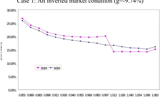
Since the trading volumes of OTM options are always larger than those of ITM options at the same strike prices, the implied volatility curve is commonly made of the implied volatilities of OTM options at each strike prices. It is well known that the skewed implied volatility curve in stock index options reflects that BSM allows the traders to adjust their fear on crash, and the skewed curve is often smooth. However, when the basis is large enough, the implied volatility curve will change a little. In other words, once the anticipation of the future spot price is formed in the futures market, the demands on the put and the call will be different, and the implied volatility curves from BSM in both cases will not be inevitable to be kink near (or at) the money, as shown in Figure 3. As for NSM, after including the compensation to price uncertainty, the values of the put and the call should be indiscriminative to the rational speculator, after which the implied volatility curve made of OTM options will naturally be smooth.

[Insert Figure 3 here]

This implies that BSM reflect that adjustments between the end-users of the put and the end-users of the call are different, and NSM reflect that the adjustments made by market makers to the put or the call are the same.

Regardless of the market condition, by the second criterion NSM is more suitable to the TXO market than BSM and a smooth volatility curve is qualified to be calibrated for further application.

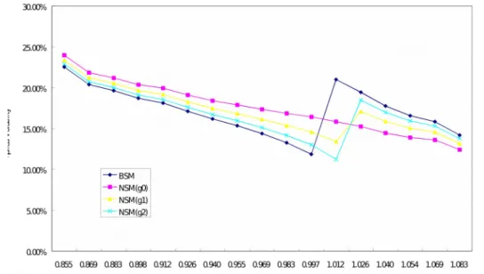
To verify that the basis is exactly the information used by the market maker to adjust his perceived volatility, we implement the similar sensitivity analysis as above and the result is showed in Figure 4. No doubt, the result is the same as that using the basis existing in the futures market is the optimal choice for the market maker

[Insert Figure 4 here]

In summary, the above observations shows that the perceived volatility

with a view, i.e. the implied volatility with the adjustment on anticipated future

spot price included in the futures market, performances good in measuring the

option value to rational speculators even when the basis between the futures and

the spot is large. This implies that when the index arbitrage in futures market

doesn’t yet start, the arbitrage in index option market does not too, even though

BSM signals an arbitrage opportunity there. Based on the above observation, we

can not deny the feature 1 with NSM.

4.2 The Calibration of the Implied Volatility Curves

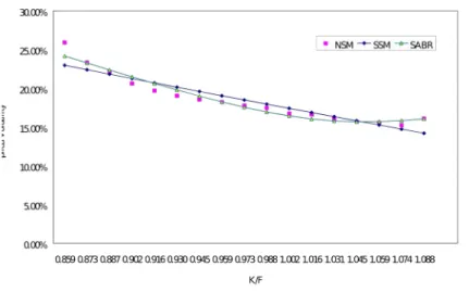
Based on the above results, we use the implied volatilities derived from NSM as the target and then showed calibrations of the implied volatility curve with the SSM and SABR models. Using the calibration with SABR is to verify the usefulness of the real-time data we choose. The calibration with SSM on this data will be used to show this model of speculation workable, and proves that the perceived volatility with a view can describe the market situation.

The results

of calibrations in both cases are shown in Figure 5. This prima facie evidence shows that the performance of SSM is a little worse than (in Case 1) or similar to (in Case 2) that of the seminal SABR model by RMSE (Root Mean of Square Error). The effectiveness of SSM shows that we can use the futures price to calibrate out a single volatility from the volatility curve. This shows that SSM improves NSM in terms of consistency and it gets the feature 2.

[Insert Figure 5 here]

4.3 The Relationship between the Anticipated Spot Price and the Perceived Volatility

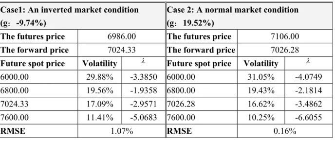
Further, SSM has a dissimilitude that could calibrate the relationship between the perceived volatility and the estimated future stock index, as shown in Table 1. We use some estimated future stock index, replacing the futures of stock index, to calibrate out the corresponding perceived volatility. Then we can see that in both extreme market cases, the lower the estimated future stock index, the higher the implied volatility derived from SSM, and vice versa. This just show that SSM possesses the feature 3 in both extreme market cases and implies that this pattern discovered in TXO market tallies with the volatility asymmetry of its underlying asset. As we use SSM to fit the skewed volatility curve and calibrated out the reverse relationship between the anticipated level of the stock index, the underlying of TXO, and perceived volatility of it, we can

16 The volatility formula provided in SABR is similar to the input of (Black, 1976) and has two inputs:

forward price and strike price. That is why one strike price, one volatility. The procedure of calibration on SSM has three steps. First, we use the formula of SSM to compute prices of OTM options on each strike prices with the futures price and an initial guessing value on the critical input: volatility. Then, we compute implied volatilities of these option prices with NSM and compare them with those of NSM. This is why the number of implied volatilities of SSM displaying in that figure is not a single one. If the deviations of these two groups of volatilities are not small enough, we try another guessing volatility in SSM and repeat the step 1. Finally, we can find an optimal volatility in SSM and that is just the resulting volatility parameter in this calibration.

say that the values of TXOs to market makers can be well measured by SSM and market makers anticipate the future average volatility of the underlying of TXOs by referring the future level of the underlying and the similar pattern existing in its spot market. This is just like a rational speculator makes his trading decision by betting on the future crowd behavior in spot market and support the destabilizing rational speculation argument proposed by (De Long et al., 1990). Since we suppose that the rational speculator plays the role of the de facto market maker, we could argue that the formation of the implied volatility skew in TXO market may be a self-fulfilling prophecy made by the rational speculator. On the other hand, we supplement (Bollen and Whaley, 2004) from the supply side of options.

[Insert Table 1 here]

5 Conclusion and Suggestion

The implied volatility of a European option derived from Black and Scholes Model is often seen as the expected average volatility during the life of the option by its traders and it should be single and equal to the future spot volatility of its underlying asset no matter what type of product it belongs and what its moneyness is.

But in reality, the existence of two well-known option- pricing puzzles – the expensiveness and the skew pattern of stock index options shows the often unjustly maligned defect of their model and thus suggests the existence of the limit of arbitrage. Although the above puzzles can be explained by the argument of the demand of options, the model-oriented studies in Behavioral Finance on the supply side of options are rare. This paper tries to investigate the formation of the second puzzle existing in TXO market based the argument of destabilizing rational speculation. The result of calibration on the real-time data adopted when the markets are approaching the limits of arbitrage is good, thus we can suggest that the speculation models designed for describing the market maker’s psychology are workable. Further we can suggest that the formation of the implied volatility skew in stock index option market may be due to the behavior of the destabilizing rational speculator when he is located in a market full of noise traders.

In the prevalence of positive feedback traders, rational speculators, the de facto market makers in this paper, will bet on the future crowd behavior. This paper supposes that the rational speculators will quote options by referring the

17 For the detail, please refer (Poon and Granger, 2003).

directional information from the futures of stock index. The perceived volatility with a view, derived from Naive Speculation Model, shows that a put and a call with the same strike are indifferent to them and they adjust the volatilities of OTM options no matter what it is a put or a call. The calibration of the volatility curve with Shifted Speculation Model shows that the self-consistency on the single volatility assumption is satisfied in this model and that the reverse relationship between the perceived volatility with a view and the anticipated future spot price, which coincides with the volatility asymmetry pattern existing in the underlying asset, TAIEX index. This is just what rational speculators will do in the prevalence of positive feedback traders. Hence, this paper suggests that the implied volatility skew in the Taiwan stock index option market may be a self-fulfilling prophecy made by the rational speculator and supplements (Bollen and Whaley, 2004) from the supply side of options.

The side product of Destabilizing Rational Speculation is that the perceived

volatility with a view can be seen naturally larger than the future realized spot

volatility. This is an explanation that this paper provides for the first volatility

puzzle. However, this need to be verified with rigorous test on the realized spot

volatility and thus it is suggested for further research.

References

Andreassen, P. and Kraus, S. (1988), “Judgmental prediction by extrapolation,”

Mimeo, Harvard University.

Barber, B.M. Lee, Y. Liu, Y. and Odean, T. (2008), “Just How Much Do Individual Investors Lose by Trading?,” Review of Financial Studies, Vol. 22, pp.609-632.

Bates, D. S. (2003), “Empirical option pricing: a retrospection,” Journal of Economics, Vol. 116, pp.387-404.

Bessembinder, H. (1992), “Systematic risk, hedging pressure, and risk premiums in futures markets,” Review of Financial Studies, Vol. 5, pp.637-677.

Black, F. (1976), “The pricing of commodity contracts,” Financial Economics, Vol. 3, pp.167-179.

Black, F. and Scholes, M.(1973), “The pricing of options and corporate liabilities,” Journal of Political Economy, Vol. 81, No. 3, pp.637-654.

Bollen, N. P. and Whaley, R. E. (2004), “Does Net Buying Pressure Affect the Shape of Implied Volatility Functions?,” Journal of Finance, Vol. LIX, No. 2, pp.711-753.

Chang, C.C., Hsieh, P.F. and Lai, H.N. (2009), “Do Informed Option Investors Predict Stock Returns? Evidence from the Taiwan Stock Exchange,” Journal of Banking and Finance, Vol. 33, pp.757-764.

Chang, C.C. Hsieh, P.F. and Wang, Y.H. (2009), “Information Content of Options Trading Volume for Future Volatility: Evidence from the Taiwan Options Market,” Working paper.

Chang, E. Chou, R. Y. and Nelling, R. Y.(2000), “Market Volatility and the Demand for Hedging in Stock Index Futures,” Journal of Futures Markets, Vol.

20, No. 2, pp.105–125.

Chatrath, A. Christie-David, R. Dhanda, K.K. and Koch, T.W.(2002), “Index futures leadership, basis behavior, and trader selectivity,” Journal of Futures Markets, Vol.22, No. 7, pp.649–677.

Chen, N. Cuny, C. J. and Haugen, R. A. (1995), “Stock volatility and the levels

of the basis and open interest in futures contracts,” Journal of Finance, Vol. 50,

pp.281-300.

De Long, J.B. Shleifer, A. Summers, L.H. and Waldmann, R.J. (1990), “Positive Feedback Investment Strategies and Destabilizing Rational Speculation,”

Journal of Finance, Vol. 45, No. 2, pp.379-395

Derman, E. and Kani, I. (1998), “Stochastic Implied Trees: Arbitrage Pricing with Stochastic Term and Strike Structure of Volatility,” International Journal of Theoretical and Applied Finance, Vol. 1, pp.61-110.

Derman, E. and Wilmott, P. (2009), “The Financial Modelers' Manifesto,”

Working paper.

Friedman, M. (1953), “The Case for Flexible Exchange Rates,” in Essays in Positive Economics by M. Friedman, University of Chicago Press.

Giot, P.(2005), “Relationships between Implied Volatility Indexes and Stock Index Returns,” Journal of Portfolio Management, Vol. 31, pp.92-100.

Hagan, P. S. Kumar, D. Lesniewski, A. S. and Woodward, D. E. (2002),

“Managing smile risk,” WILMOTT Magazine, September, pp.84-108.

Harvey, C. and Whaley, R. (1992), “Market Volatility Prediction and the Efficiency of the S&P 100 Index Option Market,” Journal of Financial Economics, Vol. 30, pp.33-73.

Haug, E. G. and Taleb, N. N.(2009), “Why We Have Never Used the Black- Scholes-Merton Option Pricing Formula,” Working paper.

Hull, J. C. (2006), Options, Futures, and Other Derivatives, (6th edition), Prentice-Hall.

Keynes, J. M. (1930), A Treatise on Money 2, Macmillan: London.

Kolb, R. W. and Overdahl, J. A., (2006), Understanding Futures Markets (6th edition), Blackwell: Oxford.

Korn, R. and Wilmott, P. (1998), “A General Framework for Hedging and Speculating with Options,” International Journal of Theoretical and Applied Finance, Vol. 1, No.4, pp.507-522.

Liu, J., and Longstaff, F. A. (2004), “Losing Money on Arbitrages: Optimal Dynamic Portfolio Choice in Markets with Arbitrage Opportunities,” Review of Financial Studies, Vol.17, No. 3, pp.611-641.

Marris, D. (1999), “Financial Option Pricing and Skewed Volatility”, Thesis of

Master Philosophy, Statistical Science, University of Cambridge.

Merton, R. C. (1973), “Theory of Rational Option Pricing,” The Bell Journal of Economics and Management Science, Vol.4, No. 1, pp.141-183.

Pan, M. S. Liu Y. A. and Roth, H. J. (2003), “Volatility and trading demands in stock index futures,” The Journal of Futures Markets, Vol. 23, No.4, pp.399–

414.

Poon, S. and Granger, C.W.J. (2003), “Forecasting Volatility in Financial Markets: A Review,” Journal of Economic Literature, Vol. XLI, pp.478-539.

Rubinstein, M.(1993), “Displaced Diffusion Option Pricing,” Journal of Finance, Vol.38, pp.213-217.

Shleifer, A. and Summers, L. (1990), “The noise trader approach to Finance”, Journal of Economic Perspectives, Vol. 4, No. 2, Spring, pp.19-23.

Shleifer, A. and Vishny, R.(1997), “The limits of arbitrage,” Journal of Finance, Vol. 52, pp.35-55.

Tavakkol, A. (2000), “Positive Feedback Trading in the Options Market,”

Quarterly Journal of Business and Economics, Vol. 39, pp.69-80.

West, G. (2005), “Calibration of the SABR Model in Illiquid Markets,” Applied

Mathematical Finance, Vol. 12, No. 4, pp.371-385.

Appendix A

(Korn and Wilmott, 1998) developed a general framework, including BS model, for using options to hedge and speculate in a basic financial market. For the readers’ convenience we roughly introduce their framework. In their paper this market consists of a bond and a risky asset with dynamics given by

t t

dB rB dt

,

(A.1)

P

t t t t

dS 





，

(A.2)

under the same regular conditions like BSM. The investor holds an option on the risky asset with a final payoff

. One thing different to BSM is that the investor can trades in the underlying and in the bond to hedge himself partly, not only “fully.” His strategy is to hold a portfolio



at time t, which is made of an option,

units of the underlying and



units of the bond. KW lets

be the subjective value of the option at time

when the underlying is

S

and assumes it to be sufficiently smooth. They also construct a portfolio

as followings.

( ) ( , ) _{t t t t}

X t V t S   S 



(A.3)

( )

X t

is the wealth process if and only if

equals to the market price of the option. Otherwise it is just the subjective belief of the wealth of the portfolio.

While the subjective belief is larger than the market price, i.e. the option is overpriced, the investor won’t like to hold the portfolio. The requirement of self- financing strategy induces to

2 2 2

2

( ) { ( ) 1 ( ( ))}

2

( )

: ( ) ( )

t t t t

t t t

t

V V V

dX t S S r V S X t dt

t S S

V S dW

S

a t dt b t dW

 



  

        

  

   



  (A.4)

where we have omitted the arguments for

. With no doubt, the terminal condition is

( , ) ( )_T

V T S  f S

(A.5)

By setting

( )

t

t

V b t S  S

   

 (A.6)

they get the general form of the partial differential equations(for short:

PDE)

2 2 2

2

1 ( ) ( ) ( )

2

V V V r

S rS rV a t rX t b t

t S S

 



   

     

   (A.7a)

( , ) ( )_T

V T S  f S

(A.7b)

This PDE is the same as Black-Scholes equation except for the right hand side of equation (A.7a). The choice of

and

depends on the investor’s goals, beliefs or strategies. Three examples in their paper related to this note are introduced as follows.

Example 1 “Full hedging”

This strategy’s feature is to the requirement of a riskless portfolio, i.e.

( ) 0

b t 

. This leads equation (A.6) to be

t

V S

  



(A.8)

For the reason of no arbitrage, they also require

. This leads the above PDE to be

2 2 2

2

1 0

2

V V V

S rS rV

t  S S

      

  

(A.9a)

( , ) ( )_T

V T S  f S

(A.9b)

This is just the same as Black-Scholes equation. The intuition behind is that the subjective value of the investor’s equals the Black-Scholes theoretical price just because his intention is purely hedging.

Example 2 “Pure speculating”

When the intention of the investor who holds an option is only for speculating, he won’t hold any stock option. Then they get

t 0

 

( ) V

b t S

S 

 



(A.10)

By requiring

they obtain

2 2 2

2

1 0

2

V V V

S S rV

t  S  S

  

   

  

(A.11a)

( , ) ( )_T

V T S  f S

(A.11b)

It is clear that the subjective value is larger than Black-Scholes price if and only if the growth rate of the underlying ^ is bigger than the riskfree rate

. An intuition behind this is that the anticipated the future spot price of the underlying will affect the demand of an call/put from the speculators in the market.

Example 3 “Partial hedging”

This example includes elements of the above two examples. Suppose that the investor can’t fully hedge the risk in his option position, but at least he can put the following constraint on the stock position.

t

V V

S S

   

  

  (A.12)

He can choose

to maximize the drift rate

and has a result like

, 0

, 0

t

V V

S if S

V V

S if S





 

 

  

      

  



(A.13)

Following the same requirement of

, the PDE is changed to

2 2 2

2 { 0} { 0}

1 ( ( )( 1 1 )) 0

2

V V V

S S r rV

t  S S   



 

 

  

      

   (A.14a)

( , ) ( )_T

V T S  f S

(A.14b)

If we have ^{ }

, this PDE agrees with Black-Scholes equation. If we have ^{ }

, it agrees with the equation of Example 2, i.e. the “pure speculating”; and further, we can deduce the same result that the subjective value is higher than Black-Scholes price when ^

if we let ^

^ .

In summary, we can see a general form of PDE derived from the example of “partial hedging”, which also includes the BSM and the “pure speculating” as special cases like

2 2 2

2

1 0

2

V V V

S yS rV

t  S S

  

   

   (A.15a)

( , ) ( )_T

V T S  f S

(A.15b)

18 For more interest cases and detailed discussion, please refer to (Korn and Wilmott, 1998).

This PDE, consisting of equation (A.8a) and (A.8b), is just the same as the

PDE consisting of equation (3a) and (3b). Depending the choice of the strategy

made by the investor, we can know the form of

. However, in this note, we

start from the Normal Backwardation theory proposed in (Keynes, 1930) and let

the derivatives markets determine the

, then measure perceived implied

volatility and further calibrate the implied volatility skew from the viewpoint of

the speculator.