動態均衡的無政府狀態價格

國立臺灣大學電機資訊學院電機工程學系 碩士論文

Department of Electrical Engineering

College of Electrical Engineering and Computer Science

National Taiwan University Master Thesis

動態均衡的無政府狀態價格

On the Price of Anarchy of Dynamic Equilibria

梁峻瑋 Jun-Wei Liang

指導教授：陳和麟 博士 Advisor: Ho-Lin Chen, Ph.D.

中華民國 110 年 1 月

January, 2021

謝 辭

首先，我發自內心地感謝陳和麟老師這一年半以來的指導。從一開始的題目上的挑選、

論文方面的選讀、開始算一些例子、猜測模型上限、直到證明模型的上限等等，研究的 每一步都是由每周例行的一對一會議指出方向，再在當周花點時間完成回家作業，並於 下周回報結果的方式來執行的。經過碩一下整個學期，持續完成這些不太費力費時的研 究作業，我的研究結果大概已經完成三分之二。而後，在碩二上學期，前半學期是完成 最後的研究，後半學期是撰寫論文的部分，最終於寒假的第二周舉行口試。我不時感嘆，

這麼愉快的研究生活就此結束，也很懷念這段順遂且具有成就感的研究旅途。

其次，我必須特別在此感謝電機系辦的承辦人員，能夠通融我形式上的繁文縟節，

幫助我處理完一連串提早口試、學位考申請、學位成績繳交等等的行政事務。也在此感 謝台大電機所在過程中多次給予的支持與協助。我誠摯地向你們說聲謝謝。

最後，感謝我的研究室同儕們在這一年半中的協力。雖然平時我們並沒有一起合作 的需求，不過整個融洽的實驗室氣氛，正是由各位所維護起來的。也感謝我的實驗室同 學，黃道譽，犧牲暑假與實習機會來努力進行研究，最終才能讓老師同意我倆一同提早 進行口試。

摘 要

在這篇論文中，我們研究了一個隨時間變化的網路流（network flow）模型，稱之為

「流體排隊模型」。考慮到一個有向圖被注入連續的流量，致使水分子傳播到每一條 邊上。對於每一條邊而言，如果流入的流率超過給定的容量，那麼超出的粒子將會 形成等待的隊伍，而其他的粒子在給定的時間長度內通過這一條邊。更精確地，我們 研究了在賽局觀點上的流體排隊模型，稱之為動態平衡模型，這被用來描述一些問 題。例子包含了網際網路、自駕車中控系統、以及中央處理器挑選任務的過程。先前，

有幾位作者研究了流體排隊模型，像是 Ford and Fulkerson [1,2]、Gale [3]、Anderson and Philpott [4]、Fleischer and Tardos [5]。 也 有 一 些 作 者 研 究 了 動 態 平 衡 模 型， 像 是 Vickrey [6]、Meunier and Wagner [7]、Cominetti, Correa, andLarré [8]、Kaiser and Marcus [9]。我們的研究延續了單調猜想 (monotonicity conjecture) 下具有常數函數流量 的網路的 PoA(Price of Anarchy) 上限結果 [10]，以及具有連續函數流量的網路的 PoA 存在性結果 [8,9]。一方面，在串並聯網路（Series­parallel network）研究 PoA 的目的 是要測量「分配任務給處理器」這項任務的無效率程度。另一方面，在具備連續函數流 量的網路研究 PoA 的目的是要縮小模型和現實中的差距。我們認為具備動態函數流量的 網路相對接近實際狀況，如自駕車中控系統。在現實生活中，交通流量隨著時間而變化。

我們在研究中發現了具備連續函數流量的網路的 PoA 上限。我們證明了平行網路和 兩層兩條邊平行網路的 PoA 上限為 2，串並聯網路有一個 PoA 上限為「網路的直徑」，

所有網路在假設成立下有一個 PoA 上限為 2|V | − 1。這是第一篇論文研究具備連續函數

流量的網路在流體排隊模型上的 PoA。我們把平行網路和串並聯網路的 PoA 上限從無限 大分別壓低到 2 和「網路的半徑」。這兩個被證明出來的上限和具備常數函數流量的網路 在流體排隊模型上的情況截然不同。另一方面，類似於在早先抽稅方案上的研究 [11]，

我們設計了一個簡單的抽稅方案來改善系統的無效率程度。這會許對於具備連續函數流 量的網路會有極大的幫助。

Abstract

In this thesis, we study a Time­Variant­Model, called the “fluid queuing model”. Consider a directed graph injected with a continuous inflow such that water propagates to each edge. For each edge, If the inflow rate exceeds the given capacity, the exceeding particles form a waiting queue, and the other particles pass through this edge under the given delay time. We study the game theory aspect of the fluid queuing model, called the dynamic equilibrium model, which was applied to describe several problems. Examples include the Internet, the self­driving car central control system, and the procedure of CPU­core.

Previously, several authors studied on fluid queuing model, likes Ford and Fulkerson [1, 2], Gale [3], Anderson and Philpott [4], Fleischer and Tardos [5]. Some authors studied on dynamic equilibrium model, likes Vickrey [6], Meunier and Wagner [7], Cominetti, Correa, andLarré [8], Kaiser and Marcus [9]. Our study continues the result of PoA bound of networks with constant inflow under monotonicity conjecture [10], and the existence of PoA of networks with dynamic inflow [8,9]. On the one hand, the purpose of studying the PoA in a series­parallel network is to measure the inefficiency of the problem of assigning tasks to processors. On the other hand, the purpose of studying the PoA of networks with dynamic inflow is to narrow the gap between the model and the reality. We think the networks with dynamic inflow will be closer to the actual situation of the central control system of autonomous vehicles. In the real world, traffic will change over time.

We find upper bounds of the PoA of networks with dynamic inflow. We prove the PoA of 2 of parallel­link networks and (2 + 2)­parallel­link networks, the PoA of “net­

work’s diameter(called D(C))” of series­parallel networks, the PoA of 2|V |−1 of general networks with assumption. This thesis is the first study on the PoA for networks with dy­

namic inflow in the fluid queuing model. That is, we reduce the upper bound of PoA

of parallel­link networks or series­parallel networks from infinite to 2 and D(C) respec­

tively. The bounds we proved are different from networks with constant inflow in the fluid queuing model. On the other hand, similar to the work of tax scheme [11], we design a simple tax scheme to improve the inefficiency of the system. This may help a lot on networks with dynamic inflow.

Contents

Acknowledges ii

Abstract in Chinese iii

Abstract in English iv

Contents vi

List of Figures viii

List of Tables ix

1 Introduction 1

2 Model 5

2.1 Fluid Queuing Model . . . 5

2.2 Flow of Model . . . 7

2.2.1 OPT flow . . . 7

2.2.2 EQU flow . . . 7

2.2.3 Throughput flow . . . 8

2.3 Networks of Model . . . 8

3 Main 10

3.1 Parallel­link Networks . . . 10 3.2 Series­parallel Networks . . . 13 3.3 (2 + 2)­parallel­link Network . . . 17

4 Extension 21

5 Conclusions and Future Works 27

References 29

Letter of Authority 31

List of Figures

2.1 The diagram of “(2 + 2)­parallel­link Network”. In the first stage C₁, the source is s and the sink is p; In the second stage C2, the source is p and the sink is t. . . . 9

3.1 The diagram of “PoA of 2 Example”. Left part is the parallel­link network with edges{e1 = (a, 0), e₂ = (1,¹₃)}; Right part is the inflow function, which is a step function with range={1, a}. . . 11

4.1 The diagram of “PoA of ⁴₃ Example” This is the parallel­link network with edges{e1 = (0.5, 0), e2 = (1, 1)}, the total amount M = 1, and the constant inflow function µ₀ = 1. . . 22 4.2 The diagram of “PoA of_e−1^e Example” This is the series­parallel­link net­

work with edges{ei = (u_i, 0), eⁱ = (uⁱ, αµ^m(_u ¹

OP T − _u¹_i))}i=1∼m, the total amount M = αµ^m, and the constant inflow function µ0 = µ^m, where m∈ N, α > 0, µⁱ =∑_i

k=1µ_k. . . 24 4.3 The diagram of “PoA of 2 Example”. Left part is the parallel­link network

with 2 edges{e1 = (a, σ), e₂ = (b, τ )}; Right part is the inflow function, which is a step function with range={1, a}. . . 25

List of Tables

1.1 Summary of result. The PoA of 2 is a tight bound of parallel­link networks and (2 + 2)­parallel­link networks; The PoA of D(C) is a loose bound of series­parallel networks; The PoA of 2|V | − 1 is a loose bound of general networks with assumption. . . 4

Chapter 1

Introduction

In this thesis, we consider the game theory aspect of the fluid queuing model proposed by Vickrey [6]. In the fluid queuing model, the system consists of a directed graph and a continuous inflow. Each edge of this graph has a capacity and a delay time. When the flow traverses through the edges, queuing occurs if the flow rate exceeds the capacity of the edge. The exceeding particles of the flow would form queuing to wait for the next moment, and the other particles would pass this edge with the delay time of edge as the cost of time. This model views each of the infinite particles as a player. These players selfishly choose the shortest path from source to sink to minimize the travel time, which forms the equilibrium flow. The travel time of each particle is the summation of the waiting time at the source plus the queuing time and delay time of each edge it chooses.

This model can be used to describe several problems. Examples include the Internet, the central control system of self­driving cars, and the task processor of the CPU core.

Consider the problem of transferring packets on the Internet. We can model the Internet as a network, packet as particle forming inflow, and network congestion as fluid queuing of each edge. On the example of traffic networks, we can model the traffic network as a network, vehicle as particle forming inflow, the traffic jam on each road as the fluid queuing of each edge. Note that the optimal solution is the self­driving car central control system. On the problem of assigning tasks to processors, we can model each processor execution time as edges of a network, the process as particle forming inflow, and the

waiting queue of each machine as the fluid queuing of each edge. In this example, the programming statements forming series operations and parallel operations, such as for­

loops or if­else. These are the motivation of series­parallel networks.

Previously, Ford and Fulkerson [1,2] provided an algorithm of the fluid queuing model with constant inflow to send the maximal mass of flow with a given time. Gale [3]

proved the existence of flow that is the optimal solution at each moment. Anderson and Philpott [4], Fleischer and Tardos [5] improved this result from each moment to continuous time version.

Consider the game theory aspect on the fluid queuing model, which is called dynamic equilibrium model and laterally introduced as “Flow of Model”, firstly studied by Vickrey [6]; Meunier and Wagner [7] proved the existence of dynamic equilibria.

For fluid queuing model with dynamic inflow, Cominetti, Correa, and Larré [8]

proved the existence of dynamic equilibria of piecewise constant inflow and locally Lebesgue­

integrable inflow. Kaiser and Marcus [9] constructively proved the existence of dynamic equilibria of locally Lebesgue­integrable inflow.

The purpose of studying the Price of Anarchy (PoA) is to evaluate and quantify the inefficiency of the system. This analysis of PoA enables us to measure each kind of game and design an improved mechanism for them. The PoA was studied in several games, likes Stackelberg game [12], selfish routing game [13], or network game or called game­

theory aspect on fluid queuing model [10]. Focusing on the networks with dynamic inflow, we discuss PoA’s bound for parallel­link networks, series­parallel networks, and general networks in this thesis. On the other hand, those two papers in the previous paragraph showed the PoA of the fluid queuing model with locally integrable inflow is finite due to the existence of dynamic equilibria.

In the fluid queuing model, the price of anarchy for networks with constant inflow is tightly bounded by _e−1^e under a weak assumption, called the monotonicity conjecture.

In particular, the price of anarchy for parallel­link networks tightly bounded by⁴₃ without any assumption [10].

Consider the existence of dynamic equilibria of locally integrable inflow and PoA’s

bound for networks with constant inflow. We want to find PoA’s bound of series­parallel networks with locally integrable inflow or called dynamic inflow. The purpose of study­

ing the PoA of series­parallel networks is related to the problem of assigning tasks to processors. That is, we want to study the efficiency of the process­and­CPU system. On the other hand, the purpose of studying the PoA of networks with dynamic inflow is to narrow the gap between the model and the reality. We think the networks with dynamic inflow would be closer to real situations, such as the internet or self­driving car central control system. In the real world, traffic will change over time.

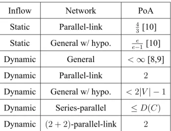
Our Result: We find upper bounds of the PoA of networks with dynamic inflow. We prove that the PoA of 2 is a tight bound for parallel­link networks and (2 + 2)­parallel­link networks; the PoA of series­parallel networks is upper bounded by D(C), where D(C) is closed related to the diameter of the network; the PoA of general networks is upper bounded by 2|V | − 1 with assumption. These results are shown in table 1.1.

This thesis is the first study on the PoA for networks with dynamic inflow in the fluid queuing model. That is, we reduce the upper bound of PoA of parallel­link networks or series­parallel networks from infinite to 2 and D(C) respectively. The bounds we proved are different from networks with constant inflow in the fluid queuing model. On the other hand, similar to the work of tax scheme [11], we design a simple tax scheme, called Delay­

time tax scheme, to improve the efficiency of the system. Surprisingly, the delay­time tax scheme did not work on networks with constant inflow but may help a lot on networks with dynamic inflow.

Our main work is to use the total amount of inflow as an upper bound of the maximal throughput of networks to afford the lower bound of the cost of optimal flows (or said optimal time) in the fluid queuing model. This technique helps us finding PoA’s tight bound of parallel­link networks and a simple example of series­parallel networks, even a loose bound of series­parallel networks. This technique provides an exactly bound of PoA of series­parallel networks with dynamic inflow. Also, it simplifies the work from finding PoA’s bound to calculating the mass of the maximal throughput of networks. On the other hand, we design a tax scheme to improve society’s welfare as a possible solution to the system’s inefficiency.

Inflow Network PoA Static Parallel­link ⁴₃ [10]

Static General w/ hypo. _e−1^e [10]

Dynamic General <∞ [8,9]

Dynamic Parallel­link 2

Dynamic General w/ hypo. < 2|V | − 1 Dynamic Series­parallel ≤ D(C) Dynamic (2 + 2)­parallel­link 2

Table 1.1: Summary of result. The PoA of 2 is a tight bound of parallel­link networks and (2 + 2)­parallel­link networks; The PoA of D(C) is a loose bound of series­parallel networks; The PoA of 2|V | − 1 is a loose bound of general networks with assumption.

Chapter 2

Model

In this chapter, there are three sections. Firstly, we will define the fluid queuing model as the base of this thesis; Secondly, we will introduce the few kinds of flows in the fluid queuing model and imply the term–the Price of Anarchy; Thirdly, we will choose some specific models to study. These contents will be used in the next chapter.

2.1 Fluid Queuing Model

Consider a network C by directed graph G = (V, E) with source s∈ V and sink t ∈ V . Each edge e_j has capacity v_j and delay time τ_j, denoted by e_j = (v_j, τ_j). Sometimes, we use the notation e_j = (a_j, σ_j). Moreover, each edge also has an infinite buffer to store the particles.

In this paper, the fluid queuing model is regarded as one of the models of network flow changes over time. The inflow of network, µ₀, is a Lebesgue locally integrable function.

Denote the last leaving time by ˆθ = sup{θ|µ0(θ) > 0}, and the total amount by M =

∫θ^ˆ

0 µ₀(θ)dθ. Here, we assume all particles have full information, enable them to imply each moment’s situation.

Let’s define fluid queuing model here, refer to [10]. For each e∈ E at θ, denote the queuing mass by z_e(θ), and the inflow rate by f_e⁺(θ), where f_e⁺(θ) : R⁺ → R⁺. At this

moment, the changing speed of z_e(θ) is:













f_e⁺(θ)− ve ↗, if f_e⁺(θ)≥ ve,

v_e− f_e⁺(θ) ↘, if f_e⁺(θ)≤ ve, z_e(θ) > 0, 0→, if f_e⁺(θ)≤ ve, z_e(θ) = 0.

So, the particle come­in e at θ will leave e at θ + z_e(θ)

v_e + τe, where ^ze_v^(θ)

e + τeis named by the travel time of e at θ.

For each e∈ E at θ + τe, denote the outflow rate by

f_e⁻(θ + τe) =





v_e, if z_e(θ) > 0, min(v_e, f_e⁺(θ)), if z_e(θ) = 0.

Now, for each v∈ V − {s, t}, no particle would stay at v at any θ. That is,

∑

e=(u,v)∈E

f_e⁻(θ) = ∑

e=(v,w)∈E

f_e⁺(θ).

For source s, particle is allowed to wait at s and leave at any θ. We have:

µ₀(θ) + ∑

e=(u,s)∈E

f_e⁻(θ)≥ ∑

e=(s,w)∈E

f_e⁺(θ),

since some particles may stay at s.

Remark 1. In the previous paper, like [10], they denote that

µ₀(θ) + ∑

e=(u,s)∈E

f_e⁻(θ) = ∑

e=(s,w)∈E

f_e⁺(θ).

But, in this thesis, we use the inequality notation. This is because we do not view the particle waiting at s as part of outflow∑

e=(s,w)∈Ef_e⁺(θ). This only has few influence on the continued part of thesis.

In the fluid queuing model, the strategy of each particle is to wait for a moment in s, and then choose a path to leave. For this particle p, the travel time is defined by waiting time at s plus the summation of the travel time of all e∈ path at the arriving time of p.

2.2 Flow of Model

2.2.1 OPT flow

The OPT solution (OPT flow) of the fluid queuing model is the strategy as below: Given network C, inflow µ₀. Each particle from µ₀ is manipulated such that the last particle can arrive at t at the earliest time. We denoted this earliest time by T_{OP T}, called the arriving time of all particles in OPT flow.

Remark 2. The OPT flow maybe not unique. We default it by the OPT flow without queuing and prefer paths with shorter delay time.

2.2.2 EQU flow

For each particle as a player, the Nash Equilibrium (EQU flow) of the fluid queuing model is the strategy as below: Given network C, inflow µ₀. For each particle, it has to choose waiting time at s plus the travel time of one of the paths from s to t. And, the cost of each particle is the arriving time. Finally, we denoted the time of the last particle arriving t by T_EQU, called the arriving time of all particles in EQU flow.

Now, let’s introduce two terms. The PoA, price of anarchy [14], is the ratio between the worst Nash Equilibrium and the optimal solution of social cost. The PoS, price of stability [15], is the ratio between the best Nash Equilibrium and the optimal solution of social cost. However, there is only one unique Nash equilibrium in this network game.

We simply denote PoA := ^T_T^EQU

OP T without any ambiguity. Here, PoA is the ratio of the arriving time of all particles in EQU flow to OPT flow.

Remark 3. The waiting time at s is 0 for all particles in this case.

Definition 1. Consider EQU flow of network C, inflow µ₀. For the particles arriving s at θ0, we denote the earliest time to arrive each v ∈ V − s by lv(θ0).

Definition 2. Consider EQU flow of network C, inflow µ₀. The mass of particle existing in C at θ₀, Q(C, µ₀, θ₀) :=∫

{θ|θ≤θ⁰,lt(θ)>θ0}µ₀(θ)dθ. When it is clear from the context, we use Q(θ₀) to denote Q(C, µ₀, θ₀).

Definition 3. ConsiderEQU flow of network C, inflow µ₀. At the moment θ₀ , we define the shortest travel time L(C, µ₀, θ₀) := l_t(θ₀)− θ0. And, at the last leaving time ˆθ, we short­write ˆL := L(C, µ₀, ˆθ). When it is clear from the context, we use L(θ₀) to denote L(C, µ₀, θ₀).

2.2.3 Throughput flow

The throughput flow of the fluid queuing model is the strategy as below: Given network C, inflow µ₀, period time θ = 0 ∼ t. Each particle from µ0 is manipulated such that sending the maximal mass of particle throughput C at inflow µ₀ during θ = 0∼ t.

Definition 4. The maximal mass of particle is denoted by M_put(C, µ₀, t). Sometimes we instead inflow function of infinite inflow rate during θ = 0∼ t to afford an upper bound of M_put(C, µ₀, t), denoted by M_put(C,∞, t). When it is clear from the context, we use M_put(t) to denote M_put(C,∞, t).

2.3 Networks of Model

Definition 5 (Parallel­link Network). Given a network C in fluid queuing model, C is Parallel­link networks if e = (s, t) for all e∈ E.

Definition 6 (Series­parallel Network). Series­parallel networks are defined by Induc­

tion: Start from parallel­link networks, each time can do series­linking or parallel­linking operation to another well­defined series­parallel network. All possible results form series­

parallel networks.

Definition 7. Given the series­parallel network C, the maximal number of each path’s nodes among all paths is denoted by D(C).

Definition 8 (Parallel­group­link Network). Given ϵ > 0 and a parallel­link network C.

If there exists [L₁, R₁], ..., [L_N, R_N], ^R_Lⁱ

i ≤ 1 + ϵ and ^L_Rⁱ⁺¹_i ≥ ¹_ϵ, and the delay time of each edge of C is in one of the intervals, then C is called parallel­group­link network.

Connected from the routing game with groups of similar links, refer to [11].

Figure 2.1: The diagram of “(2 + 2)­parallel­link Network”. In the first stage C1, the source is s and the sink is p; In the second stage C₂, the source is p and the sink is t.

Definition 9 ((2 + 2)­parallel­link Network). Given parallel­link networks C₁, C₂ and C1’s inflow µ0. Now, series­link C1 to C2, denoted by C1+ C2. Consider OPT flow and EQU flow on this linking network C₁+C₂, the maximal number of used edges in OPT flow or EQU flow in C1 and C2 part are denoted by m1 and m2 respectively. If m1, m2 ≤ 2, we called C₁+ C₂ is a (2 + 2)­parallel­link network.

Chapter 3

Main

We will show several PoA’s bounds in the fluid queuing model in this chapter. These include some tight upper bound on parallel­link networks or (2+2)­parallel­link networks and some finite upper bound on series­parallel networks.

3.1 Parallel­link Networks

First of all, we need Lemma 1 to evaluate the upper bound of the Price of Anarchy for networks.

Lemma 1. Consider the fluid queuing model with network C, inflow µ₀. For all time θ₀, if

M_put(L(θ₀))≤ k ∗ Q(θ0),

then T_EQU ≤ (k + 1) ∗ TOP T, where M_put is the maximal mass of particle throughput network, Q is the particle existing in network, and T_{OP T}, T_EQU are the arriving time of all particle in OPT flow, EQU flow respectively.

Proof. For the shortest travel time ˆL = L(ˆθ) := l_t(ˆθ)− ˆθ, we have:

T_EQU− TOP T = l_t(ˆθ)− TOP T = ˆL + ˆθ− TOP T (∗)

≤ ˆL,

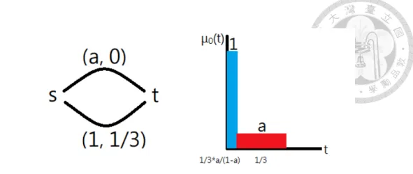
Figure 3.1: The diagram of “PoA of 2 Example”. Left part is the parallel­link network with edges{e1 = (a, 0), e₂ = (1,¹₃)}; Right part is the inflow function, which is a step function with range={1, a}.

last inequality holds by considering the leaving time and the arriving time of last particle in OPT flow. On the other hand, for the total amount M and the inequality, we have:

M ≥ Q(ˆθ) ≥ 1

kM_put(L(ˆθ))

(∗)

≥ 1

k ∗ k ∗ Mput(1 kL(ˆθ)),

last inequality holds since we can copy the infinite inflow during θ = 0 ∼ ¹_kL(ˆθ) for k times as an option of infinite inflow during θ = 0 ∼ L(ˆθ). On the other hand, since we have to send M mass of particle in OPT flow, so:

T_{OP T} ≥ 1

kL(ˆθ) = 1 k

Lˆ ≥ 1

k(T_EQU− TOP T), k + 1≥ T_EQU

T_{OP T} = PoA.

Theorem 1. In the fluid queuing model, the Price of Anarchy of 2 for parallel­link net­

works is tight.

Proof. Gien parallel­link network C, inflow µ₀, denoted e_j = (v_j, τ_j) for all e_j ∈ E. At any moment θ₀, suppose EQU flow use n edges, then we have:

L(θ₀)≤ τn+1.

For each edge, the travel time minus the delay time of edge is the queuing time. Hence, we can calculate the mass of particle queuing in C at θ0as an lower bound of Q(θ0):

Q(θ₀)≥

∑n i=1

v_i[L(θ₀)− τi],

where Q(θ₀) is the particle existing in C at θ₀. On the other hand, for each edge, the given time of M_put minus the delay time of edge is the total time to pass particle. We have:

M_put(L(θ₀)) =

∑n i=1

v_i[L(θ₀)− τi].

This implies Q(θ0) ≥ Mput(L(θ0)). Follow from Lemma 1, we have P oA ≤ 2. Fur­

thermore, let’s provide an example for the Price of Anarchy of 2. Given 1 > a > 0, consider:

E ={e1 = (a, 0), e₂ = (1,1 3)}.

µ₀(θ) =







1, θ = 0 ∼1

3 ∗ a 1− a, a, θ = 1

3∗ a

1− a ∼1 3 ∗ a

1− a + 1 3. In this case, we have:

TOP T = 1 3 ∗ a

1− a + 1 3, T_EQU = 1

3 ∗ a 1− a + 1

3+ 1 3, PoA = TEQU

T_{OP T} =

1

3 ∗ (2 − 2a + a)

1

3 ∗ (1 − a + a) = 2− a → 2 as a → 0⁺.

Theorem 2. In the fluid queuing model, if all edges in 1 aggregated network, the Price of Anarchy of 2−_1+ϵ¹ ≈ 1 + ϵ for parallel­group­link networks is tight, where ϵ is given by the network.

Proof. Given parallel­group­link network C whose edges are in 1 aggregated network, inflow µ₀, denoted e_j = (v_j, τ_j) for all e_j ∈ E. At the last leaving time ˆθ, for the shortest travel time ˆL, we have the condition:

Lˆ

τ_j ≤ 1 + ϵ, ∀ej ∈ E.

Similar as Lemma 1, we have:

T_EQU − TOP T = ˆL + ˆθ− TOP T ≤ (1 − 1

1 + ϵ) ˆL + τ₁+ ˆθ− TOP T (∗)

≤ (1 − 1 1 + ϵ) ˆL,

where the last inequality holds by considering the leaving time plus minimal delay time and the arriving time of last particle in OPT flow. Hence, we afford:

2− 1

1 + ϵ ≥ T_EQU

T_{OP T} = PoA.

Finally, similar as Theorem 1, the example for the Price of Anarchy of 2− _1+ϵ¹ is shown as below:

E ={e1 = (a,1 3

1

1 + ϵ), e2 = (1,1 3)},

µ₀(θ) =







1, θ = 0 ∼(1

3 −1 3

1 1 + ϵ) a

1− a, a, θ = (1

3 − 1 3

1 1 + ϵ) a

1− a ∼(1 3 −1

3 1 1 + ϵ) a

1− a + 1 3. In this case, we have:

T_{OP T} = (1 3 − 1

3 1 1 + ϵ) a

1− a+ 1 3, T_EQU = (1

3 − 1 3

1 1 + ϵ) a

1− a+ (1 3− 1

3 1

1 + ϵ) + 1 3, PoA = T_EQU

T_{OP T} →

2

3 −¹_31+ϵ¹

1 3

= 2− 1

1 + ϵ ≈ 2 − (1 − ϵ) = 1 + ϵ.

holding when a→ 0.

3.2 Series­parallel Networks

Lemma 2. Consider the fluid queuing model with network C, inflow µ₀, the total capacity of minimal cut face Min­Cut(C), the inequality holds:

M ≤ TOP T ∗ Min­Cut(C),

where M is the total amount and T_{OP T} is the arriving time of all particle in OPT flow.

Proof. In this case, for OPT flow, each particle from s to t has to pass by one of the edges contained in the minimal cut face of C. And, the throughput of the minimal cut face is at most Min­Cut(C) at any moment. As a result, the inequality holds.

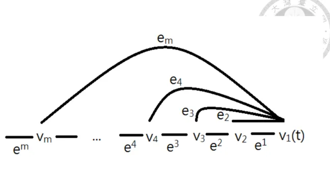
Theorem 3. In the fluid queuing model, given network C, inflow µ0. If each of C’s edge is used by OPT flow at some moment, the Price of Anarchy is at most 2|V | − 1.

Proof. At the last leaving time ˆθ, record l_v(ˆθ) for all v ∈ E − {s} and sort them into {t0, t₁, ..., t_n}. We discretize the earliest travel time ˆL = lt(ˆθ)− ˆθ into interval (ti−1, t_i).

Note that, n + 1≤ |V |.

We know that (t_i−1, t_i) contains some edges with some queue mass. For each edge e_j in this interval, we suppose e_j start at t_{f (j)} ≤ ti−1, denoted e_j = (v_j, τ_j) and the queuing mass z_j(t_{f (j)}), then:

z_j(t_{f (j)})

v_j + τ_j ≥ ti− ti−1.

Now, for network C, interval (t_i−1, t_i), consider the Min­Cut(C) and an index set of interval S :={k|ek ∈ [ti−1, ti]}, we have:

∑

k∈Sz_k(t_{f (k)})

∑

k∈Sv_k ≤ M

∑

k∈Sv_k ≤ M Min­Cut(C)

(∗)

≤ TOP T,

last inequality holds by Lemma 2. This implies min_k∈S ^zk(t_v^{f (k))}

k ≤ TOP T. Now, consider j = arg min^zk(t_v^{f (k))}

k , we have:

ti− ti−1 ≤ ^zj(t_v^{f (j)}_j ⁾+ τj (∗)

≤ TOP T + TOP T, L = L(C, µˆ 0, ˆθ) = lt(ˆθ)− ˆθ = tn− t0 =∑n

i=1ti− ti−1 ≤ 2n ∗ TOP T, PoA≤ 2n + 1 = 2|V | − 1.

Note that, τ_j ≤ TOP T holds since OPT flow uses all edges including e_j.

Conjecture 1. In the fluid queuing model, removing each OPT­unused edge in networks only worsens the Price of Anarchy. Hence, the Price of Anarchy is at most 2|V | − 1 for networks.

Remark 4. In parallel­link networks, this conjecture is true. In general networks, this conjecture could be false, take Pigou’s example for an example. The conjecture is possible to be true in series­parallel networks.

Theorem 4. In the fluid queuing model, the Price of Anarchy is at most D(C) for series­

parallel networks C, where D(C) denotes the maximal number of each path’s node among all s to t paths.

Claim: Given a series­parallel network C, inflow µ₀, any moment θ₀. For the through­

put flow M_put, the shortest travel time L, and the mass of particle existing in network Q.

We have the inequality:

M_put(C,∞, L(C, µ0, θ₀))≤ (D(C) − 1)Q(C, µ0, θ₀), which implies the Theorem from Lemma 1.

Proof. (a)Base Case

In parallel­link network, D(C) = 2. The statement is true by Theorem 1.

(b)Parallel­linking

After parallel­linking operation, series­parallel networks C₁ links to C₂. For C’s inflow µ₀, define the EQU flow’s inflow of C₁ is µ^up₀ , inflow of C₂ is µ^dn₀ , and µ₀ = µ^up₀ + µ^dn₀ ; for any moment θ₀. we have:

L(C₁, µ^up₀ , θ₀) ≥ L(C, µ0, θ₀), L(C₂, µ^dn₀ , θ₀) ≥ L(C, µ0, θ₀),

Q(C, µ₀, θ₀) = Q(C₁, µ^up₀ , θ₀) + Q(C₂, µ^dn₀ , θ₀).

Induction hypothesis of Claim:

given C₁, µ^up₀ , θ₀ : M_put(C₁,∞, L(C1, µ^up₀ , θ₀))≤ (D(C1)− 1)Q(C1, µ^up₀ , θ₀), given C₂, µ^dn₀ , θ₀ : M_put(C₂,∞, L(C2, µ^dn₀ , θ₀))≤ (D(C2)− 1)Q(C2, µ^dn₀ , θ₀),

This implies:

M_put(C,∞, L(C, µ0, θ₀))

(∗)

≤ sum of LHS

≤ sum of RHS

≤ max(D(C1)− 1, D(C2)− 1)[Q(C1, µ^up₀ , θ₀) + Q(C₂, µ^dn₀ , θ₀)]

= (D(C)− 1)Q(C, µ0, θ₀),

where D(C) = max(D(C₁), D(C₂)). And, the first inequality holds since the throughput of C is just the sum of throughput of C₁and C₂ with same period time.

(c)Series­linking

After series­linking operation, series­parallel networks C₁ links to C₂. For C₁’s inflow µ₀, define the EQU flow’s outflow of C₁is µ₁, and µ₁is C₂’s inflow; for any moment θ₀, define θ₁ = l_p(θ₀). We have:

L(C, µ₀, θ₀) = l_t(θ₀)− θ0

= l_t(θ₀)− θ1+ l_p(θ₀)− θ0

= L(C₂, µ₁, θ₁) + L(C₁, µ₀, θ₀),

Q(C, µ₀, θ₀)

(∗)

≥ Q(C1, µ₀, θ₀), Q(C, µ₀, θ₀)

(∗∗)

≥ Q(C2, µ₀, θ₀).

Inequality (*) holds by consider the mass of particle existing in C1 at θ = θ0 as a lower bound; Inequality (**) holds by consider the mass of particle existing in C₂at θ = θ₁as a lower bound.

Induction hypothesis of Claim:

given C₁, µ₀, θ₀ : M_put(C₁,∞, L(C1, µ₀, θ₀))≤ (D(C1)− 1)Q(C1, µ₀, θ₀), given C₂, µ₁, θ₁ : M_put(C₂,∞, L(C2, µ₁, θ₁))≤ (D(C2)− 1)Q(C2, µ₁, θ₁),

This implies:

M_put(C,∞, L(C, µ0, θ₀))

(∗)

≤ sum of LHS

≤ sum of RHS

≤ [D(C1)− 1 + D(C2)− 1]Q(C, µ0, θ₀)

= (D(C)− 1)Q(C, µ0, θ₀),

where D(C) = D(C1) + D(C2)− 1. Moreover, the first inequality holds since we can consider C₂sending infinite particle without delay time in θ = 0∼ θ1and C₁sending infinite particle without delay time in θ = θ1 ∼ lt(θ0) as an upper bound of Mput.

3.3 (2 + 2)­parallel­link Network

Remark 5. We remove all edges exceed m₁ and m₂, where m₁ and m₂ are the maximal number of used edges in OPT flow or EQU flow in C₁ and C₂ parts respectively. And, this has no influence on our model. On the other hand, we use e_j = (a_j, σ_j) in C₁ and e_j = (v_j, τ_j) in C₂.

Now, consider the flows on network C₁ and inflow µ₀. Define T_EQU|C1,T_{OP T}|C1 as the arriving time of all particle in EQU flow and OPT flow respectively. Let’s see a new model named by ”Restricted Inflow Model” as below:

Definition 10 (Restricted Inflow Model). In EQU flow, consider any moment θ₀such that µ0(θ0) ≥ a1 + ... + am1 and lt(θ0) = σm1. We imitate the OPT flow, let µ0(θ0)− (a1 + ... + a_m1) mass of particles wait at s until µ₀ ≤ a1+ ... + a_m1 and all previous particles have leaven.

In EQU flow after the operation, the arriving time of each particle is the same as usual.

Since the order of any pair of particles is conserved and each edge passing the same mass of particles as usual. Furthermore, the travel time of each particle is at most σ_m1 in the Restricted inflow model. Finally, each particle in EQU flow would depart earlier or equal to OPT flow, since there is always no more particle wait at s in EQU flow.

Definition 11 (Different Arriving Time). Given parallel­link network C₁, inflow µ₀, each particle p from µ₀. Define d(C₁, µ₀, p) by the different arriving time of EQU flow to OPT flow for particle p. Define d(C₁, µ₀) = sup_pd(C₁, µ₀, p).

Follow from definition, we have:

d(C1, µ0, p)≤ σm1. TEQU|C1 − TOP T|C1

(∗)

≤ d(C1, µ0)≤ σm1,

last inequality holds by considering the last particle as a special case of particle p.

Definition 12 (EO flow). Given (2 + 2)­parallel­link network C1 + C₂, inflow µ₀. For EQU flow in network C₁ using inflow µ₀, we have the outflow of C₁ as the inflow of C₂,

denoted by µ₁. Now, consider the OPT flow of network C₂using inflow µ₁, this is the EO flow in (2 + 2)­parallel­link network C₁+ C₂. And, define the arriving time of all particle in EO flow by the arriving time of all particle in OPT flow of network C₂using inflow µ₁.

Define n₂ is the maximal number of used edges in EO flow or EQU flow in C₂part.

We apply the above lemma on networks C₂, inflow µ₁, we have:

T_EQU − TEO ≤ τn2 ≤ τm2,

where And, m₂ is the maxiaml number in OPT flow or EQU flow in C₂ part. Since we remove all edges exceed m₂, n₂ ≤ m2.

Lemma 3. In the fluid queuing model, given (2 + 2)­parallel­link network C₁ series­

linking to C2 and inflow µ0, denoted ej = (aj, σj) in C1 and ej = (vj, τj) in C2. For the OPT flow and EQU flow, we have:

T_EQU − TOP T ≤ σm1 + τ_m2.

Proof. Follow from above, for the EO flow in this (2 + 2)­parallel­link network, we have:

T_EQU− TEO ≤ τm2, T_EQU|C1 − TOP T|C1 ≤ σm1.

In EO flow, consider a strategy as below: For all particle arriving source of C₂, let them wait at source for σm1 − d(C1, µ0, p) time and leave. In this case, EO flow has the same inflow of C₂as OPT flow, but delay for exactly σ_m1 time. That is:

OPT’s inflow of C₂ : µ₂(θ), EO’s inflow of C₂ : µ₂(θ + σ_m1),

where µ₂(θ) is the inflow of C₂in OPT flow. This relationship implies T_EO−TOP T = σ_m1. However, EO flow may choose some better solutions, implies

T_EO− TOP T ≤ σm1,

T_EQU − TOP T = T_EQU− TEO+ T_EO− TOP T ≤ σm1 + τ_m2.

Remark 6. Inthe proof of Lemma 3, for EO flow, we let the particle wait at the intermedi­

ate point p. Despite this is not allowed in our model, it only worsens T_EQUand makes the PoA bigger. The upper bound of PoA is still true if we allowed waiting at the intermediate point p. So, we allow it.

Lemma 4. Given (2 + 2)­parallel­link network C₁+ C₂, T_{OP T} = T_EOor T_{OP T} ≥ σ2+ τ₂, where T_{OP T}, T_EOis the arriving time of all particle in OPT flow and EO flow respectively and (a₁, σ₁), (a₂, σ₂) denotes the edges of C₁, (v₁, τ₁), (v₂, τ₂) denotes the edges of C₂.

Proof. Given (2 + 2)­parallel­link network C₁ + C₂, inflow µ₀, the maximal number of used edges in OPT flow or EQU flow in C₁ part and C₂ part are m₁ and m₂ respectively.

Now, if m₁ = 1, then T_{OP T} = T_EO. Else, consider m₁ = 2. Let’s divide it into two cases:

(a)m₁ = 2 and a₁ ≥ v1

During θ = 0 ∼ σ2, OPT flow and EO flow have the same inflow and outflow at C₂. Now, if m₂ = 1, after θ = σ + 2, OPT flow and EO flow still have the same outflow at C₂, implying T_{OP T} = T_EO. Else, m₂ = 2, both OPT and EO active (v₂, τ₂) at θ = σ₁.

• If EO flow shutdown (v₂, τ₂)f irst, then T_EO ≤ TOP T, implies T_EQ = T_{OP T}.

• If OPT flow shutdown (v₂, τ₂)f irst but before θ = σ₂+ τ₂, then OPT flow and EO flow have the same outflow at C₂ later, which will pass the same mass of particle.

We let EO flow shutdown (v₂, τ₂) at the same time to afford T_EQ = T_{OP T}.

• If OPT flow shutdown (v₂, τ₂)f irst and after θ = σ₂+ τ₂, then T_{OP T} ≥ σ2+ τ₂.

(b)m₁ = 2 and a₁ ≤ v1

If m₂ = 1, consider the EO flow and OPT flow. Maybe EO flow and OPT flow have the total same outflow, then T_EO = T_{OP T}; Else, EO flow and OPT flow must have the same outflow during θ = 0∼ σ2+ τ₁, implies T_{OP T} ≥ σ2 + τ₁. Both of the cases are enough to prove PoA≤ 2.

Else, m₂ = 2, which implies a₁+ a₂ ≥ v2 ≥ a1 since v₂is used. Now, if OPT flow

use (v₂, τ₂), then T_{OP T} ≥ σ2+ τ₂. Else, EQU flow use (v₂, τ₂), we can compute:

M_put(C,∞, σ2 + τ₂) =













0, θ = 0 + τ₁ ∼ σ1+ τ₁, a₁(σ₂ − σ1), θ = σ₁ + τ₁ ∼ σ2+ τ₁, v₁(τ₂− τ1), θ = σ₂ + τ₁ ∼ σ2+ τ₂.

M_put(C, µ₀, σ₂+ τ₂) =















0, θ = 0 + τ₁ ∼ σ1+ τ₁,

∫ _σ2−σ1

0

min(µ₀(θ), a₁)dθ, θ = σ₁+ τ₁ ∼ σ2+ τ₁, v₁(τ₂− τ1), θ = σ₂+ τ₁ ∼ σ2+ τ₂. On the other hand, in EQU flow, let’s find a lower bound of the total mass of particle arriving at the source of C₁+ C₂ before activating (v₂, τ₂) as an lower bound of M :











0, θ = 0 + τ1 ∼ σ1+ τ1,

the mass of particle passing by C₁+ C₂ =∫_σ2−σ1

0 min(µ₀(θ), a₁)dθ, θ = σ₁+ τ₁ ∼ σ2+ τ₁, the mass of particle queuing at C2to active (v2, τ2) = v1(τ2− τ1), θ = σ2+ τ1 ∼ ˆθ.

As a result, we have:

M_put(C, µ₀, σ₂+ τ₂)≤ M.

Similar as Lemma 1, this implies T_{OP T} ≥ σ2+ τ₂.

Theorem 5. In the fluid queuing model, the Price of Anarchy of 2 for (2 + 2)­parallel­link networks is tight.

Proof. Follow from the Lemma 4, if T_{OP T} = T_EO, apply Lemma 1 on network C₂using inflow µ₁, we have:

T_EQU

T_{OP T} = T_EQU T_EO ≤ 2.

On the other hand, if T_{OP T} ≥ σ2+ τ₂, together with Lemma 3, we have:

TOP T ≥ σ2+ τ2 ≥ TEQU − TOP T, PoA = ^T_T^EQU

OP T ≤ 2.

So, we achieve the goal.

Chapter 4

Extension

We will show a self­defined tax scheme and improve the PoA’s bound with it in the fluid queuing model. Although it seems helpless for the networks with constant inflow, it is helpful for the parallel­link networks with some extreme inflow cases.

Definition 13 (Delay­time Tax Scheme). In the fluid queuing model, we increase the delay time of edges by imposing tax in the given networks. The tax is not considered as the cost of society’s welfare. That is, the tax scheme will only change the behavior of particles, and the computation of delay time and travel time still uses the original setting. This is called the delay­time tax scheme, refer to [11].

Remark 7. Under the definition of the Delay­time Tax Scheme, OPT flow would not change anything after taxing. This is because the computation of delay time and travel time still uses the original setting. As a result, we only discuss EQU flow and the changes on the arriving time of all particle in EQU flow, T_EQU.

Theorem 6. In the fluid queuing model with constant inflow, the Price of Anarchy is at least ⁴₃ for parallel­link networks after taxing.

Proof. Let’s show an example of the Price of Anarchy of ⁴₃, refer to [10]. Consider the parallel­link network with two edges, the total amount M , and the constant inflow function