應用射流於霧社水庫底泥清淤: 以小模型實驗進行可行性評估與研究

(1)

I

國立臺灣大學工學院土木工程學系碩士論文

Department of Civil Engineering College of Engineering

National Taiwan University Master Thesis

應用射流於霧社水庫底泥清淤:

以小模型實驗進行可行性評估與研究

Jet-aided venting of cohesive sediment deposits from Wushe Reservoir: feasibility study using small-scale experiments

古涵山

Salah H. Khadeeda 指導教授：卡艾瑋教授 Advisor: Dr. Hervé Capart

中華民國 100 年 7 月 July, 2011

(2)

II

(3)

I

ACKNOWLEDGMENTS

I would like to thank all people who have helped and inspired me during my master study.

I especially want to thank my advisor, Prof. Hervé Capart, for his guidance during my research and study at National Taiwan University. His perpetual energy and enthusiasm in research had motivated all his advisees, including me. In addition, he was always accessible and willing to help his students with their research. As a result, research life became smooth and rewarding for me.

I would like thank to all my lab mates at the MorphoHydraulic Research Group Laboratory for their help and friendship in the past two years. In particular, I would like to thank Prof. Hervé Capart’s PhDs students (Ke-Wen Tao, Ni-Wei Jie and Steven Lai) for them advices and guides for Code writing and experiments. For inspiring me in research and life through our interactions during the long hours in the lab, made it a convivial place to work.

I especially want to thank Prof. J. S. Lai and his research team, for providing data and Wushe reservoir’s experimental model at Nanshijiao Experiment Laboratory.

I would like to thank technician at Geotechnical Laboratory, Civil Engineering Department, for providing all experiment tools and guiding me during soil analysis experiment.

Best regards and thanks to all my friends in Taiwan, to all Taiwanese people, whose always kind and helpful to me during undergraduate and graduate study in Taiwan. Special thanks to National Taiwan University for supporting, patience, and teaching me the brilliant knowledge.

My deepest thanks and gratitude goes to my family, to my parents, to my brothers and sisters for their unflagging love and support throughout my life; this thesis is simply impossible without them. Finally want to thank all my friends in Iraq for their encouragement and support.

(4)

II

ABSTRACT

In this thesis, field investigation and laboratory experiments are performed to investigate the feasibility of underwater jetting as an aid to reservoir de-siltation. For understanding jetting and underwater dredging technique, we reviewed ROVs’ technology, undersea trenching technique and dredging platform-boat of Shimen Reservoir. Wu-She Reservoir was selected as reference filed case. We reviewed current plan of developing dam, collected samples from the bottom of reservoir and analyzed its characteristics. Small-scale 1D experiment, were conducted to observe cohesive bed response to point-jet. In this experiments, a driven carriage to move an oblique point-jet along a horizontal bed of cohesive Wu-She Reservoir’s soil. The resulting jetting flow, trench shape and turbid cloud are observed from the side using a digital camera, and from the top using a medical ultrasound probe. The laboratory model is used to measure trench shapes for a range of jet flow rates and advancing speed. The depth and advancing speed for our cohesive silt-mud mixture are then compared to pervious experimental measurements for non-cohesive sand. Next we conducted experiments on 2D laboratory model to scale 1:1000 of Wu-She Reservoir. To compare the efficiency of sediment venting with and without jetting. A first set of experiments was conducted in a 1D narrow channel. Then, a second set of experiments was conducted in 2D channel. For 2D model Sinlaku typhoon data’s was selected as an initial condition for the set of experiments. Then concluding our thesis simulating topography of reservoir before and after flood event to observe venting outlet’s efficiency aided by point-jet.

Keywords: underwater dredging; jet trenching; reservoir; sedimentation; cohesive bed; medical ultrasound; topography.

(5)

III 摘要

本篇論文結合現場調查和實驗室實驗探討水下清淤技術，包括噴射挖溝和分散機制反應在高凝聚力底泥上，觀察水下凝聚力底床的地貌變化。為了瞭解噴射和水下清淤技術，我們回顧了 ROV 的技術，海底挖溝清淤技術和石門水庫抽泥船.對於噴射流技術應用在水庫底泥上.我們選定了霧社水庫做為野外研究對象。因此我們回顧它目前霸體改建的計畫, 採樣水庫底泥的樣本和分析它的特性是必需的。在一維小尺模型實驗，觀察噴射流反應在有高凝著力姓底泥和底床縱段面的改變。我們使用可以控制履帶來移動一個噴嘴且沿著水平底床深的噴嘴射流。引起的水流，渾濁的濃度以及溝渠的切割與形狀被觀察到從側面使用數位相機，從上面使用醫術的超音波。此模型用來測量溝渠的形狀由於不同的流量的射流以及移動速度。溝渠的深度，射流流量以及移動速度，以有凝聚力性的泥土一起以前沒凝聚力的材料實驗測量之結果比較。之後用二維 1 比 1000 的霧社水庫模型，來模擬與量測俳沙口的小流。第一組實驗是颱風的時候只開俳沙口，第二組實驗首先用射流噴底床的底，

颱風進入水庫後才開拍沙口，在二維實驗，我們選了辛樂克颱風的資料與 2007 霧社水庫的長剖面當初始條件。使用地形掃描的量側與進入和出濃度，來比較不同實驗的結果。從結果來決定射流應用在清淤霧社水庫的淤積底泥。

關鍵字: 水下淸淤; 噴射挖溝; 水庫; 沉積; 凝聚力姓的底床; 醫術的超音波; 地形掃描

(6)

IV

LIST OF FIGURES

Figure 1-1. Geographical location of Wu-She Reservoir. (Courtesy of S.Y.J. Lai) ...2

Figure 1-2. 3D view of Wu-she Reservoir, showing upstream Choushui River is the mainstream for Reservoir. (SAT-2) ...3

Figure 1-3. Three views of Wu-she Dam: dam outflow gate, intake and divergence tunnel, spillway slope. ...6

Figure 1-4. Satellite image of Wu-she Reservoir, illustrating different water levels influence front travelling delta’s topset. (SAT-2 image collected and organized by Ke W.T.) ...8

Figure 1-5. Forest bed profiles of Wu-she Reservoir from 1995 to 2010. (Source: Taiwan Power Company) ...9

Figure 1-6. Influence of the deposition volume to the capacity volume of Wu-she Reservoir from 1995 to 2009. (Source: Taiwan Power Company) ... 10

Figure 1-7. Schematic image for improving dam project. (Source: Sinotech Engineering Consultants Company) ... 12

Figure 1-8. Dredging platform-boat of Shimen Reservoir. (by Prof. H.Capart) ... 14

Figure 1-9. Water-jets of dredging platform-boat of Shimen Reservoir. (by Prof. H.Capart) ... 14

Figure 1-10. Undersea Burying cable or pipes mechanism. [Sand bed response to the action of moving jet. [A.T.H Perng and H. Capart] ... 15

Figure 1-11. Jet-trencher. (Photo by J.F. Vanden Berghe,Fugro Engineering) ... 16

Figure 1-12. Idealized schematic view for applying water-jet technique to Reservoir. ... 18

Figure 2-1. Turbidity current phenomena. ... 20

Figure 2-2. Taking samples from up stream’s surface water. ... 20

Figure 2-3. Satellite Image of the Wushe-Resevoir (took on 2009.12.13) yellow and red dots identifying the location of the sampling stations were collected in different time. ... 21

Figure 2-4. Fish Finder and Portable GPS... 22

Figure 2-5. Platform Boat Used for collecting sample. (provided by Wu-she Reservoir) ... 22

Figure 2-6. Show the phleger sampler by (Ke, W. T. & Kh. Salah). ... 23

Figure 2-7. (Left) everyone wear preserver jacket, (right) arranging rope and hoisting plug & chain. ... 25

Figure 2-8. Recording GPS coordinate position and water depth of the sampling station. ... 27

Figure 2-9. Throwing sampler vertically to the bottom. ... 27

(9)

VII

Figure 2-10. Pulling sampler by rope by ( Kh.Salah & Ke, W.T.). ... 28

Figure 2-11. Taking inner tube vertically and covering it by rubber stopper. ... 28

Figure 2-12. Marking each sample and put vertically in a box. ... 29

Figure 2-13. Heating pycnometer and shaking it in the same time, to saturate all soil. ... 31

Figure 2-14. (up-left) weighting a certain amount of soil (up-right) 100ml of Hexametaphosphate solution for 50gm of soil (down-left) dispersing soil and solution (down- right) Reading hydrometer. ... 32

Figure 2-15. Particle-size distribution curve-hydrometer analysis of each sample. ... 33

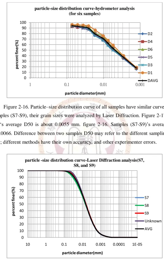
Figure 2-16. Particle–size distribution curve of all samples have similar curve. ... 34

Figure 2-17. Shows the grain size curve of samples (S7, S8 and S9). ... 34

Figure 2-18. Settling velocity of different particle diameter’s size. ... 35

Figure 2-19. (Left) liquid limit apparatus, (right) liquid limit determination... 38

Figure 2-20. Flow curve for liquid limit determination of soil... 39

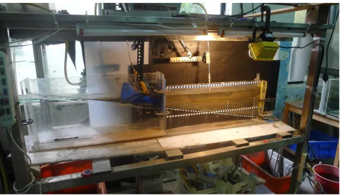
Figure 3-1. Photo and sketch of small-scale laboratory experiment tank. ... 41

Figure 3-2. Small-scale jetting tools. ... 42

Figure 3-3. high-pressure 0.5 hp water pump. ... 43

Figure 3-4. Side view of advancing machine. ... 43

Figure 3-5. Top view of advancing machine. ... 44

Figure 3-6. Particle-size distribution curve analysis of Wu-she Reservoir material. ... 44

Figure 3-7. SONIX ultrasound acoustic system. ... 45

Figure 3-8. Sequence photos of depth formation-time exposure for similar layers. ... 46

Figure 3-9. Sequence photos of depth formation-time exposure for non-similar layers. ... 47

Figure 3-10. Observed depth formation of static nozzle for similar layers of soil. ... 48

Figure 3-11. Observed depth formation with static nozzle for non-similar layers of soil. ... 48

Figure 3-12. Depth exposure time curve. ... 49

Figure 3-13. The sequence photo under flow rate Q=2.2 ml/s and advancing speed U=0.2 cm/s. ... 51

Figure 3-14. The sequence photo under flow rate Q=3 ml/s and advancing speed U=0.2 cm/s. .. 52

Figure 3-15. Depth due flow rate Q=2.2 ml/s and advancing speed U=0.2 cm/s ... 53

Figure 3-16. Depth due depth due flow rate Q=3 ml/s and advancing speed U=0.2 cm/s... 53

(10)

VIII

Figure 3-17. Depth due to different flow rate Q and advancing speed U for Wu-she Reservoir

materials. ... 55

Figure 3-18. Depth due to different flow rate Q and advancing speed U for non-cohesive sand [by Chiun-Chau Su]. ... 55

Figure 3-19. Comparison of depth due to different flow rate Q and advancing speed U for two different materials. ... 56

Figure 3-20. (Left) cavity shape for cohesive bed. (Right) cavity shape for non-cohesive bed [ by Ke-Wen Tao]. ... 57

Figure 3-21. by moving point jet (left) observing cohesive bed interfaces. (Right) observing non- cohesive bed interfaces [Chiun-Chau Su]. ... 57

Figure 3-22. Sequence photos of cavity formation by ultrasound machine. ... 59

Figure 4-1. Photo and schematic image of small-scale laboratory experiment tank. ... 61

Figure 4-2. Simulating affection of the flood event to the bed level of the dam area without opening any venting outlets except surface outlet for remaining study state condition. For scenario A. ... 62

Figure 4-3. Simulating affection of the flood event to the bed level of the dam area within opening venting outlets and surface outlet. For Scenario B. ... 63

Figure 4-4. Simulating and observing affection of dispersed dam’s bottom by jet-trenching tool then coming flood event and opening bottom-venting outlet, observing different in the bed level before and after flood even plus jet-trenching. For scenario C. ... 63

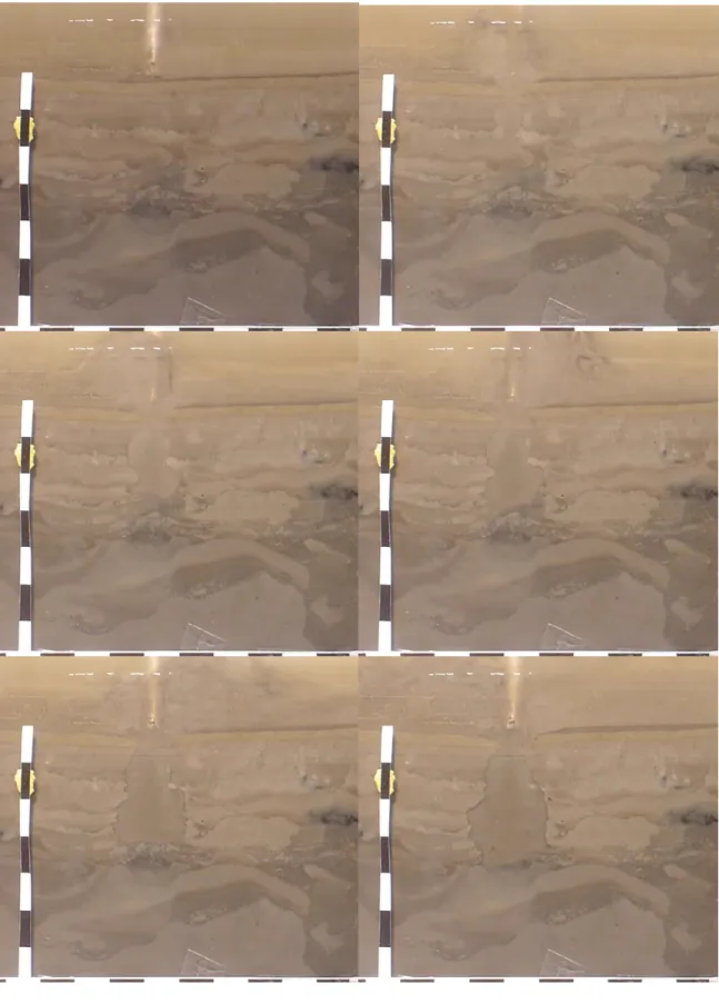
Figure 4-5. sequnce of photography for secnario A. ... 67

Figure 4-6. sequnce of photography for secnario B. ... 71

Figure 4-7. sequnce of photography for secnario C. ... 77

... 80

Figure 4-9. Concentration by weight of scenario A’s runs. ... 80

Figure 4-10. Concentration by weight of scenario B’s runs. ... 81

Figure 4-11. Concentration by weight of scenario C’s runs. ... 82

Figure 4-12. sediment discharge of three runs of scenario A. ... 83

Figure 4-13. sediment discharge of three runs of scenario B. ... 84

Figure 4-14. sediment discharge of three runs of scenarios C... 85

Figure 4-15. Different on bed level before and after flood event for Scenario A. ... 88

(11)

IX

Figure 4-16. Different on bed level before and after flood event for Scenario B. ... 90

Figure 4-17. Different on bed level before and after point jet dispersing and flood event for Scenario C... 91

Figure 5-1. Experiment model. ... 93

Figure 5-2. Process for preparing experiment’s sediment. ... 94

Figure 5-3. Process for setting up point jet tools. ... 95

Figure 5-4. upstream flow rate and sediment concentration for Wu-she Reservoir during typhoon. (Source: The team of Dr. J. S. Lai of The Hydrotech Research Institute) ... 97

Figure 5-5. upstream flow rate and sediment concentration for laboratory model experiment during typhoon. (Source: The team of Dr. J. S. Lai of The Hydrotech Research Institute) ... 97

Figure 5-6. Upstream inflow and sediment inflow rate for laboratory model experiment. (Source: The team of Dr. J. S. Lai of The Hydrotech Research Institute) ... 98

Figure 5-6. Shows the bed level condition of the model. ... 104

Figure 5-7. A, B and C upstream delta’s level and shape of scenario A, B and C. ... 105

Figure 5-8. A, B and C downstream overflow condition of scenario A,B and C. ... 107

Figure 5-9. Experiment’s process for scenario A. ... 108

Figure 5-10. Experiment’s process for scenario B... 109

Figure 5-11. Point-jet’s process of scenario C... 111

Figure 5-12. Schematic image of the jetting path for reservoir. ... 111

Figure 5-13. Experiment’s process for scenario C... 112

Figure 5-14. Scanning system’s devices. ... 113

Figure 5-15. Calibration target... 114

Figure 5-16. Adjusting calibration target and laser sheet, clicking on the calibration points from images. ... 115

Figure 5-17. Cartesian coordinate of calibration target. ... 116

Figure 5-18. Distance and position of each marker. ... 117

Figure 5-19. Relation between photo names and its correlated position in x direction. ... 117

Figure 5-20. Catching laser line from image. ... 118

Figure 5-21. Transferred 3D lines. ... 119

Figure 5-22. shaded DTM. ... 119

(12)

X

Figure 5-23. Drying oven and concentration pan’s samples………133

Figure 5-24. Comparison between inflow concentration and out flow concentrations of scenario A, B and C. ... 120

Figure 5-25. topgography of Wu-She Reservoir model, before and after flood event for scenario A. ... 123

Figure 2-26. topgography of Wu-She Reservoir model, before and after flood event for scenario A (with a different color scale analysing the bottom near the dam). ... 124

Figure 5-27. Long profile of scenario A before and after flood event by taking minimum points of each section. ... 125

Figure 5-28. Long profile of scenario A before and after flood events by taking average points of each section. ... 125

Figure 5-29. topgography of Wu-She Reservoir model, before and after flood event for scenario B. ... 126

Figure 5-30. topgography of Wu-She Reservoir model, before and after flood event for scenario B (with a different color scale analysing the bottom near the dam). ... 127

Figure 5-31. Long profile of scenario B before and after flood events by Minimum points of each section. ... 128

Figure 5-32. Long profile of scenario B before and after flood events by average points of each section. ... 128

Figure 5-33. topgography of Wu-She Reservoir model, before and after flood event for scenario C. ... 129

Figure 5-34. topgography of Wu-She Reservoir model, before and after flood event for scenario C (with a different color scale analysing the bottom near the dam). ... 130

Figure 5-35. Long profile of scenario C before and after flood events by taking minimum points of each section. ... 131

Figure 5-36. Long profile of scenario C before and after flood events by taking average points of each section. ... 131

Figure 5-37. 1D laboratory experiment model. ... 132

Figure 5-38. 2D laboratory experiment model. ... 132

Figure 5-39. Scenario A’s results for 1D and 2D laboratory experiment model. ... 133

Figure 5-40. Scenario B’s results for 1D and 2D laboratory experiment model. ... 134

(13)

XI

Figure 5-41. Scenario C’s results for 1D and 2D laboratory experiment model. ... 135

Figure 5-42. Comparing view of reservoir after typhoon for laboratory model Wu-She Reservoir. ... 136

Figure 5-43. Comparing view of upstream for laboratory model Wu-She Reservoir. ... 137

Figure 5-44. Comparing sediment transport‘s view for laboratory model and Wu-She Reservoir. ... 137

Figure 5-45. Long profiles before and after typhoon for laboratory model and Wu-She Reservoir. For experiment (top figure), the venting outlet is opened. For the field, no venting outlet yet exists. ... 138

Figure 6-2. Path of the point-jet. ... 139

Figure 6-2. Bed-long profile before and after typhoon. ... 140

Figure 6-3. Bed-topography before and after typhoon. ... 140

Figure 6-4. Large scale experiment. ( by K,W.T.) ... 142

Figure 6-5. High-pressure water pumps and jet system. (by H.Capart) ... 142

Figure 6-6. Dual-frequency identification sonar (DIDSON) system has 1.1 MHz and 1.8 MHz operation frequency. The longest detective distance is about 30 m. It can be operated in the 300 m depth. (by Ke,W.T.) ... 143

(14)

XII

LIST OF TABLES

Table 1-1. Basic information of the Wu-she Reservoir’s dam. ...4

Table 2-1. TWD97-GPS and Abscissa Coordinate Position of Sampling Station. ... 21

Table 2-2. Shows the Specific Gravity of the samples. ... 30

Table 2-3. Laboratory record table of the hydrometer analysis test of (six samples). ... 36

Table 2-4. Laboratory record table of PL, LL and PI of (six samples). ... 38

Table 2-5. Porosity of the samples. ... 39

Table 3-1. Shows depth different flow rate, advancing speed... 54

Table 4-1 concentration by weight of scenario A’s runs. ... 79

Table 4-2 concentration by weight of scenario B’s runs. ... 80

Table 4-3 concentration by weight of scenario C’s runs. ... 81

Table 4-4 sediment discharge of scenario A’s runs. ... 86

Table 4-5 sediment discharge of scenario B’s runs. ... 86

Table 4-6 sediment discharge of scenario C’s runs. ... 86

Table 5-1. Dimensions used in set-upping experiment. ... 96

Table 5-2. prototype field information of Sinlaku Typhoon for Wu-she Reservoirs. (Source: The team of Dr. J. S. Lai of The Hydrotech Research Institute) ... 99

Table 5-3. Sinlaku typhoon information for laboratory model. (Source: The team of Dr. J. S. Lai of The Hydrotech Research Institute) ... 101

Table 5-4. Outlet concentration for scenario A. ... 121

Table 5-5. Outlet concentration for scenario B. ... 121

Table 5-6. Outlet concentration for scenario C. ... 121

(15)

1

Chapter 1 Background and Objectives

To know the description and properties of the field, getting more information and be more familiar with the study site, researchers need to have clear description and explanation of the investigation area, during last two years. I did several visiting to the Wu-she Reservoir and getting information from different units, to have a sufficient panorama.

1.1 Study area Site information

Wu-she Reservoir (also called Wanda reservoir or Green Lake) was built by Taiwan Power Company in 1960, located in Wu-she River, a tributary of Choshui River at Ren-ai Township at Nantou County in the central of Taiwan. Figure 1-1 and 1-2. Watershed area of the reservoir is 219 square kilometer, length of the backwater is 7.9 main the elevation 1005 m is the highest water level. Figure 1-3 and Table 1-1. Main purposes of constructing are regulating flow path in downstream, power generator and drinking water.

(16)

2

Figure 1-1. Geographical location of Wu-She Reservoir. (Courtesy of S.Y.J. Lai)

(17)

3

Figure 1-2. 3D view of Wu-she Reservoir, showing upstream Choushui River is the mainstream for Reservoir. (SAT-2)

(18)

4

Table 1-1. Basic information of the Wu-she Reservoir’s dam.

Wu-She Dam

Type of dam Arched gravity dam

Elevation of dam EL. 1005.84 m

Height of dam 114 m

Crest length of dam 205 m

Spillway structure

(a) Spillway on the top of dam

Elevation of weir 998.9 m

Max flood discharge 850 cms

(b) Outlet of dam

Elevation of outlet centre EL. 927.65 m

(c) Divergence tunnel

Elevation of intake weir 989.759 m

Power generation intake

Elevation of intake EL. 738.48 m

Max power generation discharge 24 cms

(19)

5

(20)

6

Figure 1-3. Three views of Wu-she Dam: dam outflow gate, intake and divergence tunnel,

spillway slope.

Review of sedimentation history in Wu-she Resevoir

Wu-she Reservoir was built by the experience and assistance from American Bureau of Reclamation. The engineers designed the reservoir for one hundred years life, however they didn’t consider sedimentation issue, and therefore venting outlet of the dam was built for that era’s Taiwan geological and climate changes condition. After 921 (Chi Chi) earthquakes on 1999, which caused weakness on the geological condition of the entire island due to the ruptured fault, therefore rate of the sediment value dropping to the reservoir was increasing year by year. Vast forward traveling of the delta due to the decreasing of water level and massive growing-up of the bed level of the reservoir started from last ten years. Figure 1-4 and 1-5.

(21)

7

(22)

8

Figure 1-4. Satellite image of Wu-she Reservoir, illustrating different water levels influence front travelling delta’s topset. (SAT-2 image collected and organized by Ke W.T.)

(23)

9

Figure 1-5. Forest bed profiles of Wu-she Reservoir from 1995 to 2010. (Source: Taiwan Power Company)

Long profile of Wu-She Reservoir from 1995 to 2010

940 950 960 970 980 990 1000 1010

0 500 1000 1500 2000 2500 3000 3500 4000 4500 5000

Distance (m)

Elevation (m)

1995 1996 1997 1998 1999 2000 2001 Jul-03 Nov-03 Dec-05 Nov-06 Nov-07 Aug-09 2010

(24)

10

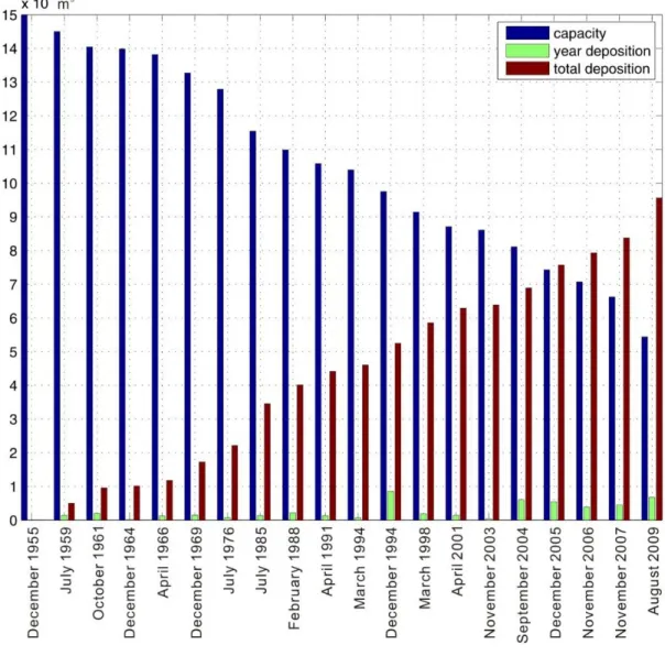
Originally total capacity of the reservoir was 148.6 million square meters, but until Dec.2009 there were 95.6 million square meters, which capacity is less than half of the total capacity and continuously deposition lead the reservoir capacity decreasing dramatically, specially after typhoon Sinlaku, damaged the function of generating power energy. Figure 1-6.

Figure 1-6. Influence of the deposition volume to the capacity volume of Wu-she Reservoir from 1995 to 2009. (Source: Taiwan Power Company)

(25)

11

Current plan of Wu-she Reservoir

According to Taiwanese engineers’ perspective and models simulating, deposition of sediment will reach to the dam in next ten years. In 2009 Taiwan power company within consulting and advising of the Sinotech Engineering Consultants Company, proposed some methodology for controlling sedimentation, opening drainage channels for flowing away sediment from upstream and downstream during floods and typhoons. Other methodology is improving the function of the dam by opening four venting outlet. Figure 1-7, for venting out deposited mud and fine sediment in front of the dam during floods.

(In front view)

EL 980

(26)

12 (Side view)

Figure 1-7. Schematic image for improving dam project. (Source: Sinotech Engineering Consultants Company)

EL 970 EL 981 EL 999.70 EL 1005

(27)

13

1.2 Jetting technology used in Shimen Reservoir

Shimen Reservoir (northern of Taiwan), has became increasingly affected by sedimentation.

According to the [Northern Region Water Resources Office]’s data ,annually about 2,120,000 cubic meter of sediment deposit in the reservoir, but currently annual dredging volume of sediment is 1.130,000 cubic meter, still there is volume of 990,000 cubic meter of sediment deposit on the reservoir.

For maintaining intakes and increasing PRO’s venting efficiency, that will increase water capacity and somehow decrease sedimentation in front of the dam. Shimen reservoir used jet- trenching mechanism for underwater engineering. In 2008 start to construct suction-dredger carried by platform boat within high pressure pump. Figure 1-8 and 1-9. they used jet-trenching for dispersing front-intakes mud and dredging or flushing out during floods, annually flushing and de-silting volume of sediment by PROs and Power Generator outlets, totally volume is 700,000 cubic meter. Dredging by suction-dredger boat platform total volume is 400,000 cubic meter of mud per year, dredging mechanism economically very expensive and need fund, but for removing dam area deposited sediment have very efficient result.

(28)

14

Figure 1-8. Dredging platform-boat of Shimen Reservoir. (by Prof. H.Capart)

Figure 1-9. Water-jets of dredging platform-boat of Shimen Reservoir. (by Prof. H.Capart)

(29)

15

1.3 Jet trenching technology

Another source of inspiration for the present thesis is the reheology used to excavate trenching under the sea. Figure 1-10. Shows the erosion of underwater sand beds and cable burial by jet trenching tools, moved along the sea bottom using ships or remotely operated vehicle (ROVs).

Figure 1-10. Undersea Burying cable or pipes mechanism. [Sand bed response to the action of

moving jet. [A.T.H Perng and H. Capart]

(30)

16

Many tools used in costal and marine engineering, such as dredging by suction for transferring sediment to other area by belt-stepper, this method is used for reclaiming new land in costal area.

Figure 1-11. Shows the vehicle which is carried all the trenching tools including high-power, pressures pumps and surveying equipments.

Figure 1-11. Jet-trencher. (Photo by J.F. Vanden Berghe,Fugro Engineering)

(31)

17

1.4 objective

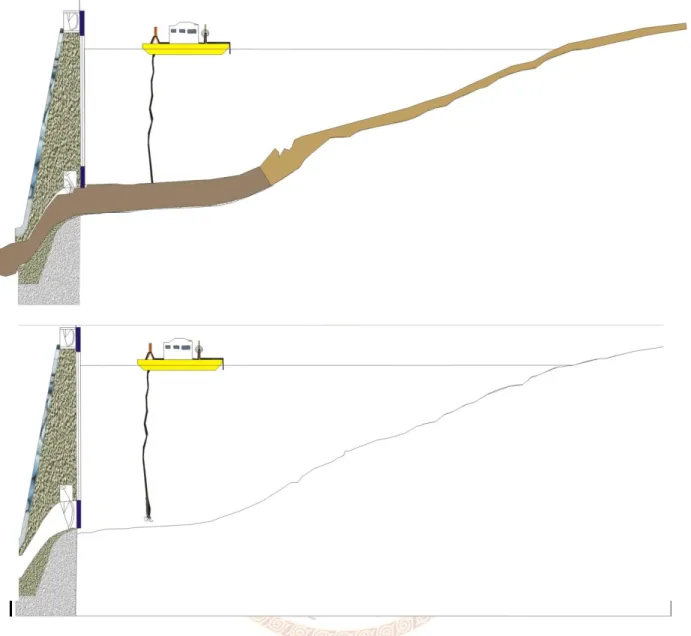
To address sedimentation problem in Wu-She Reservoir, one of the plans considered by Taipower Company is to open a venting outlet through the dam. The elevation for this outlet is referenced at EL 970, which is the level of reservoir’s bed. According to simulations by Sinotech Consultants, venting will decrease the accumulation of mud and sediment during flood.

My objectives to increase the efficiency of venting, the approach I wish to test in this thesis is to conduct pre-flood jetting of reservoir deposits. In this way, it is hoped that suspended deposits can be vented together with new sediment influx when the vent is operated under high flow. To perform the jetting operation, it is suggested to use high speed jets driven by powerful pumps like those used by the Shimen dredging boat or by jet trencher ROVs. Figure 1-12.

(32)

18

Figure 1-12. Idealized schematic view for applying water-jet technique to Reservoir.

For analyzing and proving my methodology, we need to research and do experiments, therefore for achieving the objective, this thesis contents to five chapters, first chapter exploring study area and reviewing jet-trenching technology, second chapter investigating on the Wu-she Reservoir’s material characterizations and its properties, chapter three and four focusing on the single jet characterization and its application on the 1D flume. Chapter five presents 1/1000 Wushe- Reservoir, physical model tests, for three different scenarios experiments. Finally, conclusion are drown.

(33)

19

Chapter 2 Material Sampling and Characterization

The purpose of this chapter is to identify and describe procedures and protocols for sediment sampling and testing. The sediment characteristics of interest include D50, specific gravity, plasticity and fall velocity. This is especially important because we will use actual filed material from Wu-She Reservoir is conducting the laboratory experiments.

2.1 Sampling Location

Surface sampling

Figure 2-1. Shows turbidity phenomena in the upstream. In order to measure sediment concentration, we collect the sample by inserting the bottle upside-down into the water. Rotate the open end toward the direction of the flow, and allow the bottle to fill under the surface.

Figure 2-2. Laboratory result yield that the upstream sand concentration C is weight of the dry fine sand to the total weight and it is (0.014~0.055).

Bottom sampling

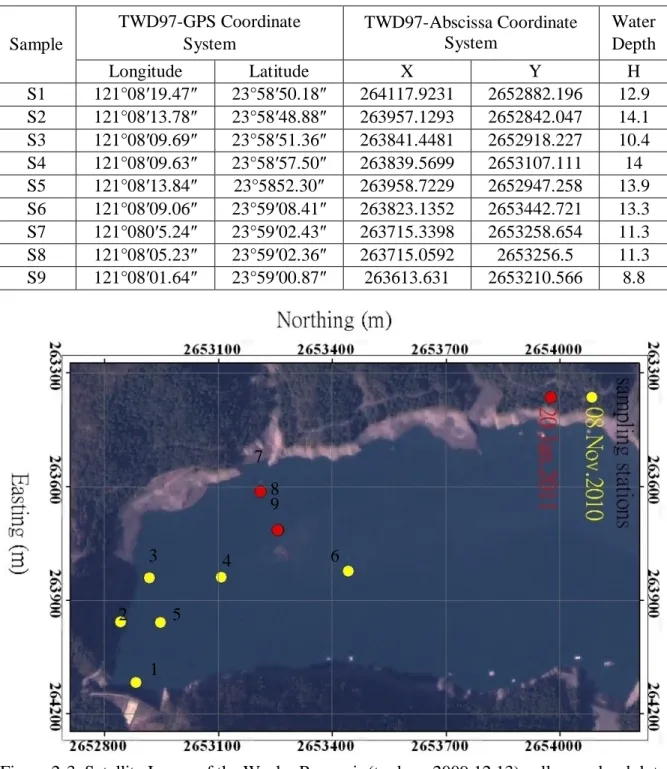
We planned to take samples from the deep bottom of downstream near the intakes and dam, Pre-

monsoon samplings (S1 to S6) were carried out in 08 November 2010, while post-monsoon samplings (S7 to S9) were carried out in 20 January 2011, and all samples were collected by (NTU MorphoHydraulics Research Group & Hydrotech Institute). During sampling Wu-She Reservoir’s most high water level was about (~983m). The locations of the sampling stations, in coordinates, were predetermined and their positions identified on site using portable Global Positioning System (GPS) and Fish Finder. Figure 2-3. Fare distance between each two samples is about (100 m-200 m). Figure 2-4. And table 2-1. Shows samples stations and coordinates .We used pontoon platform boat without fence, this kind of boat is more flexible and match to our purpose. Worked by engine, platform was (2.7 m) wide and (6.5 m) long, which is offered by Wushe-Reservoir‘s managing office. Figure 2-5.

(34)

20

Figure 2-1. Turbidity current phenomena.

Figure 2-2. Taking samples from up stream’s surface water.

(35)

21

Table 2-1. TWD97-GPS and Abscissa Coordinate Position of Sampling Station.

Sample

TWD97-GPS Coordinate System

TWD97-Abscissa Coordinate System

Water Depth

Longitude Latitude X Y H

S1 121°08′19.47″ 23°58′50.18″ 264117.9231 2652882.196 12.9 S2 121°08′13.78″ 23°58′48.88″ 263957.1293 2652842.047 14.1 S3 121°08′09.69″ 23°58′51.36″ 263841.4481 2652918.227 10.4 S4 121°08′09.63″ 23°58′57.50″ 263839.5699 2653107.111 14 S5 121°08′13.84″ 23°5852.30″ 263958.7229 2652947.258 13.9 S6 121°08′09.06″ 23°59′08.41″ 263823.1352 2653442.721 13.3 S7 121°080′5.24″ 23°59′02.43″ 263715.3398 2653258.654 11.3 S8 121°08′05.23″ 23°59′02.36″ 263715.0592 2653256.5 11.3 S9 121°08′01.64″ 23°59′00.87″ 263613.631 2653210.566 8.8

Figure 2-3. Satellite Image of the Wushe-Resevoir (took on 2009.12.13) yellow and red dots identifying the location of the sampling stations were collected in different time.

1 2

4 6

8

3

5

7 9

(36)

22

Figure 2-4. Fish Finder and Portable GPS.

Figure 2-5. Platform Boat Used for collecting sample. (provided by Wu-she Reservoir)

(37)

23

2.2 Sampling and analysis

Phleger gravity sampler are most desirable in order to collect thin surface layer of bottom’s sediments .this sampler’s weigh is about 20 kg within additional lead weights and have a core tube of diameter 3.5 cm and length 80 cm. Figure 2-6. The top part of the corer has fins for stabilization and an area for adding weights to increase penetration. A valve assembly at the top of the coring tube consists of a tapered bung that can slide in two directions to up during descent to allow water to flow through thereby decreasing the bow wave and down during ascent to form a seal on the tapered tube seating and thus prevent washout and aid in sample retention (source:

underwater soil sampling, testing, and construction control). This sampler is handy and most convenient for investigation. its generally deployed from a boat to sample soft to sandy and muddy sediments material in dam or lake that deep (10 m-20 m), for Wu-she Reservoir (~15 m) were the deepest.

Figure 2-6. Show the phleger sampler by (Ke, W. T. & Kh. Salah).

(38)

24

Equipments

-Boat.

- Life preserver jacket.

-Rope.

-Phleger gravity sampler.

-Polycarbonate transparent tubes.

-Fish Finder and its portable battery.

-Portable GPS.

-Record papers and marker.

-Digital camera.

Safety

When working on water, either in a boat, float or platform. Figure 1-7. There is some important rules should be considered:

Always wear life preserver jacket. Always have a boat available when working on a float or platform. Keep platform and working areas free of excess tools and equipments. Use adequate anchor and securing lines (we tight rope with very heavy stone and dropped to water) and check them form time to time to assure proper tension. Be sure your body is clear of all lines before dropping sampler and never straddle sampler line. Mark these lines length, so they can easily notify the depth of the water. Always clean the way of the boat form floating woods, for the boat’s engine safety. Always avoid from the Fish Net Stockings, which settled by local fishers.

After finishing work return everything to its original place and follow all rules and regulations set by reservoir community.

(39)

25

Figure 2-7. (Left) everyone wear preserver jacket, (right) arranging rope and hoisting plug &

chain.

Procedures

The procedures of collecting bottom sediments by phleger sampler are following:

Step 1 Preparation of phleger sampler:

1. Insert a polycarbonate transparent tube in the corer body.

2. Attach a lead weight on the corer. Because the bottom sediment is muddy therefore this weight is enough for getting more than 50 cm depth sample.

Step 2 Collection of sample:

1. Determining the depth of the sampling station by using fish-finder tool. Figure 1-8.

2. Selecting appropriate rope, tie one end of a rope to the bottom of the sampler and the other end to boat.

3. Throw the sampler vertically carefully and let it sink down freely to the bottom. Figure 1- 9.

4. After settling down on the bottoms, pulls the sampler smoothly back on board, and keep the bottom-up position not to loose the collected sediment core in the tube of the corer.

Figure 1-10.

5. Take the outer tube out gently, then take the inner tube from outer one very carefully and holding up in the vertical position then immediately cover the bottom and upper very

(40)

26

tightly by rubber cover, to prevent the leaking and evaporation of the surface water.

Figure 1-11.

6. Stick a note paper on the tube, and write down the coordinate of position, time and any other notes on it.

7. Vertically place the tube in box to prevent from mixing sediment layer. Figure 1-12.

8. Repeating all above procedures for taking samples from other locations.

(41)

27

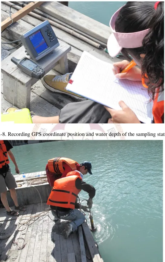
Figure 2-8. Recording GPS coordinate position and water depth of the sampling station.

Figure 2-9. Throwing sampler vertically to the bottom.

(42)

28

Figure 2-10. Pulling sampler by rope by ( Kh.Salah & Ke, W.T.).

Figure 2-11. Taking inner tube vertically and covering it by rubber stopper.

(43)

29

Figure 2-12. Marking each sample and put vertically in a box.

(44)

30

2.3 Laboratory Analysis

One month was devoted to analyzing soil sampled from the field. All geotechnical tests were done at the NTU Geotechnical Laboratory. Some of the steps were prepared with help by Yeh, C.H. And by students’ of the fall 2010 capstone course.

Specific gravity test (G)

The pycnometer method was used for determining the specific gravity of solid particle of the very fine grained soil showed in. Table 2-2 and Figure 1-13. The specific gravity of solids is determined using the relation:

(1)

Where M1=mass of empty Pycnometer, M2= mass of the Pycnometer with dry soil M3= mass of the Pycnometer and soil and water, M4 = mass of Pycnometer filled with water only.

Table 2-2. Shows the Specific Gravity of the samples.

Sample Gs

S1 2.755

S2 2.767

S3 2.761

S4 2.757

S5 2.767

S6 2.759

(45)

31

Figure 2-13. Heating pycnometer and shaking it in the same time, to saturate all soil.

Grain Size Analysis (Sieve and Hydrometer Analysis

)

for sample (S1-S6), putting soil in sieves, all soil passed sieve 200#(00.075mm), except wood’s ash, which is less than 1g, its ignored according to ASTM. Figure1-14. For this reason we used hydrometer analysis method for yielding particle distribution curve, Figure 1-15.

In this test following formula had been used:

Where t is in minute and D is given in mm, Calculation of the equivalence particle diameter is:

(2)

And calculation of the percent finer:

(3)

Where (T in min., D in mm, L, r, a and Ws in gram), is time, diameter, effective depth, correction factor and weight of the soil sample.

(46)

32

Figure 2-14. (up-left) weighting a certain amount of soil (up-right) 100ml of Hexametaphosphate solution for 50gm of soil (down-left) dispersing soil and solution (down-

right) Reading hydrometer.

(47)

33

Figure 2-15. Particle-size distribution curve-hydrometer analysis of each sample.

0 20 40 60 80 100

0.001 0.01

0.1 1

percent finer(%)

particle diameter(mm)-log scale particle-size distribution curve-

hydrometer analysis S1

0 20 40 60 80 100

0.001 0.01

0.1 1

percent finer (%)

particle diameter (mm)-log scale particle-size distribution curve-

0 20 40 60 80 100

0.001 0.01

0.1 1

percent fine(%)

hydrometer analaysis S3

0 20 40 60 80 100

0.001 0.01

0.1 1

percent finer(%)

particle diamter (mm)-log scale particle-size distribution curve-

0 20 40 60 80 100

0.001 0.01

0.1 1

percent finer(%)

particle diameter (mm)-log scale particle-size distribution curve-

0 20 40 60 80 100

0.001 0.01

0.1 1

percent finer(%)

(48)

34

Figure 2-16. Particle–size distribution curve of all samples have similar curve.

For samples (S7-S9), their grain sizes were analyzed by Laser Diffraction. Figure 2-17. samples (S1-S6)‘s average D50 is about 0.0055 mm. figure 2-16. Samples (S7-S9)’s average D50 is about 0.0066. Difference between two samples D50 may refer to the different sampling stations location; different methods have their own accuracy, and other experimenter errors.

Figure 2-17. Shows the grain size curve of samples (S7, S8 and S9).

0 10 20 30 40 50 60 70 80 90 100

0.001 0.01

0.1 1

percent finer(%)

particle diameter(mm)

particle-size distribution curve-hydrometer analysis (for six samples)

D2 D4 D6 D5 D3 D1 DAVG

0 10 20 30 40 50 60 70 80 90 100

1E-05 0.0001

0.001 0.01

0.1 1

10

percent finer(%)

particle diameter(mm)

particle -size distribution curve-Laser Diffraction analysis(S7, S8, and S9)

S7 S8 S9 Unknown AVG

(49)

35

Fall velocity

Because particle size of Wu-she reservoir’s bottom soil is very small, therefore we used hydrometer analysis test, to determine fall velocity of the particles. The suspension of particles within a fluid is governed by Stokes law

(4)

Where V is the settling velocity, d is the particle diameter, m is the density difference between the particle and the fluid, and is the viscosity of the fluid. from Figure 2-8 and Table 2-3. shows that the settling velocity of the particle is very slow and take long time to settle down, for D50 particle size, settling velocity is about 0.03 mm/s, if we assume that we have 0.5 m deep water, and put it one particle of D50 size, it will take around 5 hours to settle on the bottom of the tank.

Figure 2-18. Settling velocity of different particle diameter’s size.

0 1 2 3 4 5 6

0.001 0.01 0.1 1

settling velocity(mm/s)

particle diamter (mm)-log scale

settling velocity & particle diameter relation (six samples)

v2 v4 v6 v5 v3 v1 VAVG

(50)

36

Table 2-3. Laboratory record table of the hydrometer analysis test of (six samples).

particle size analysiz

Gs=2.7554 a=0.98

test No. 1 experimentor SALAH date 11月24日 Dry soil weight 50gm

date time last(min) r rw temp. 'C R=r-rw L(cm) D (mm) P % K n*0.001 v m/s v mm/s

11月24日 15:15:00 0 4.4 21.4 -4.4 16.29 #DIV/0! -8.624 0.013 0.98 #DIV/0! #DIV/0!

15:15:30 0.25 53 4.1 21.5 48.9 7.598 0.0717 95.844 0.013 0.98 0.005012952 5.013 15:16:00 0.5 52.9 4.1 21.5 48.8 7.6144 0.0507 95.648 0.013 0.98 0.002511886 2.5119 15:17:00 1 52.5 4.1 21.5 48.4 7.68 0.036 94.864 0.013 0.98 0.001266763 1.2668 15:18:00 2 51.9 4.1 21.5 47.8 7.7784 0.0256 93.688 0.013 0.98 0.000641497 0.6415 15:21:00 5 48 4.1 21.5 43.9 8.418 0.0169 86.044 0.013 0.98 0.000277698 0.2777 15:31:00 15 42.8 4.1 21.5 38.7 9.2708 0.0102 75.852 0.013 0.98 0.000101944 0.1019 15:46:00 30 38.5 4.1 21.7 34.4 9.976 0.0075 67.424 0.013 0.97 5.53293E-05 0.0553 16:16:00 60 34 4 21.8 30 10.714 0.0055 58.8 0.013 0.97 2.96655E-05 0.0297 19:26:00 250 24.2 3.9 22.5 20.3 12.321 0.0029 39.788 0.0129 0.97 8.02456E-06 0.008 11月25日 15:15 1440 13.3 3.8 22.6 9.5 14.109 0.0013 18.62 0.0128 0.97 1.59279E-06 0.0016

Gs=2.767 a=0.98

test No. 2 experimentor SALAH date 11月23日 Dry soil weight W=50gm

date time last(min) r rw temp. 'C R=r-rw L(cm) D (mm) P % K n*0.001 v m/s v mm/s 11月23日 11:30:00 0 52.7 5.2 20 47.5 7.6472 #DIV/0! 93.1 0.01325 1.002 #DIV/0! #DIV/0!

11:30:15 0.25 52.5 4.5 22 48 7.68 0.07172076 94.08 0.01294 0.97 0.005098156 5.0982 11:30:30 0.5 51 4.5 22 46.5 7.926 0.05152005 91.14 0.01294 0.97 0.002630728 2.6307 11:31:00 1 50.5 4.5 22 46 8.008 0.03661814 90.16 0.01294 0.97 0.001328972 1.329 11:32:00 2 49.5 4.5 22 45 8.172 0.02615673 88.2 0.01294 0.97 0.000678095 0.6781 11:35:00 5 44 4.9 21.9 39.1 9.074 0.01737817 76.636 0.0129 0.97 0.000299317 0.2993 11:45:00 15 39.1 4.5 21.9 34.6 9.8776 0.01046815 67.816 0.0129 0.97 0.000108608 0.1086 12:00:00 30 34.6 4.2 21.9 30.4 10.616 0.00767364 59.584 0.0129 0.97 5.83614E-05 0.0584 12:33:00 60 30.1 4.15 21.9 25.95 11.354 0.00561152 50.862 0.0129 0.97 3.12094E-05 0.0312 15:40:00 250 22 4.1 22 17.9 12.682 0.00291446 35.084 0.01294 0.97 8.4186E-06 0.0084 11月24日 11:30 1440 12.1 4 22.7 8.1 14.306 0.00126583 15.876 0.0127 0.97 1.58809E-06 0.0016

Gs=2.761 a=0.98

test No. 3 experimentor SALAH date 11月24日 Dry soil weight 50gm

date time last(min)r rw temp. 'C R=r-rw L(cm) D (mm) P % K n*0.001 v m/s v mm/s

11月24日 15:03:00 0 4.5 21.4 -4.5 16.29 #DIV/0! -8.82 0.013 0.98 #DIV/0! #DIV/0!

15:03:15 0.25 52.1 4.5 21.4 47.6 7.7456 0.07242 93.296 0.013 0.98 0.0051357 5.1357 15:03:30 0.5 52 4.5 21.4 47.5 7.762 0.05126 93.1 0.013 0.98 0.00257329 2.57329 15:04:00 1 50.9 4.5 21.4 46.4 7.9424 0.03667 90.944 0.013 0.98 0.00131655 1.31655 15:05:00 2 49.5 4.5 21.4 45 8.172 0.0263 88.2 0.013 0.98 0.0006773 0.6773 15:09:00 5 43.5 4.4 21.4 39.1 9.156 0.01761 76.636 0.013 0.98 0.00030354 0.30354 15:19:00 15 39.2 4.4 21.5 34.8 9.8612 0.01054 68.208 0.013 0.98 0.00010881 0.10881 15:34:00 30 33.9 4.1 21.5 29.8 10.73 0.00777 58.408 0.013 0.98 5.9199E-05 0.0592 16:04:00 60 29.5 4.1 21.8 25.4 11.452 0.00567 49.784 0.013 0.97 3.1817E-05 0.03182 19:14:00 250 22.8 3.9 22.5 18.9 12.551 0.00288 37.044 0.0129 0.97 8.202E-06 0.0082 11月25日 15:04 1440 12.7 3.8 22.6 8.9 14.207 0.00128 17.444 0.0129 0.97 1.6119E-06 0.00161