單分子量測系統與關聯分析之應用

國立台灣大學理學院物理研究所 博士論文

Department of Physics College of Science

National Taiwan University Doctoral Dissertation

單分子量測系統與關聯分析之應用

Applications of Single-Molecule Spectroscopy and Correlation Analysis

楊禮綾

Li-Ling Yang

指導教授：范文祥 博士 董成淵 博士 Advisor : W.S. Fann, Ph.D C.Y. Dong, Ph.D

中華民國 98 年 6 月

June, 2009

To my beloved family and my mentor for life

Dr. Wunshain Fann 1961 ~ 2008

~ You can have a successful career in science, academic world.

A very important thing is : Do be afraid to look like a fool. ~

中文摘要

單分子測量術近年來受到廣泛的應用，尤其在生物分子的構形、動態與其動力學的 研究上。系綜測量下無法獲得的資訊，如:總體分佈及變異，則可藉由單一分子的觀 察而得。本篇論文的工作旨在建立單分子光學實驗系統及方法，及其相關應用，主 要涵蓋兩大部分：

1. 泛素之動態構形研究 – 單分子螢光能量移轉光譜學

2. 時間相關螢光光譜學與單光子探測技術之應用 – 共軛高分子、螢光奈米鑽 石、生物分子與微流體混合器

單分子螢光能量移轉光譜學為一奈米尺度下丈量尺規，其能量移轉效率與兩標定染 間的距離變化有極大的關聯。透過染料分子的標定，生物分子的構形變化與動態則 會反映在螢光能量移轉效率的變化。觀測系統主要為共焦顯微鏡，根據實驗的需要 將生物分子固定與玻片表面或於溶液中直接觀測。另一方面，我們亦由螢光光子資 料的擷取與分析上著手，透過螢光關聯分子與光子-光子間時距的紀錄獲得額外的資 訊，並成功的應用於其他相關實驗上。這些努力主要是爲蛋白質早期摺疊過程之研 究而準備，希望能結合快速混合微流體元件、螢光關聯分析與螢光能量移轉光譜以 解析摺疊動態。

Abstract

Single-molecule detections have been known for the potential to provide additional information beside ensemble measurements. Population heterogeneities and synchronous (or asynchronous) reaction pathways pertaining to conformational dynamics and molecular interactions are veiled by ensemble averaging. The scope of this thesis is to establish general experimental methodologies on the basis of single-molecule detection, and the applications have been covered as well. The frame of this work is mainly composed of two parts:

1. Conformational dynamics of ubiquitin are investigated by spFRET (single-paired Förster Resonance Energy Transfer).

2. Applications of TCSPC (Time-Correlated Single Photon Counting) and FCS (Fluorescence Correlation Spectroscopy) on conjugated polymers, FND (Fluorescence Nano Diamond), biomolecules and micro-fluidics.

FRET serves as a distance ruler in close proximity (~ 1 nm to ~ 10 nm), and dynamic changes in structure of proteins can be thus recorded accurately. We have established optical methods to observe ubiquitin molecules either immobilized on the cover-slip surface or in free solution. On the other hand, detections based on single photon counting and correlation analysis has also been applied for further information aside from intensity analysis. At the same time, a continuous-flow micro-fluidic mixer is under development, which has claimed sub-ms mixing dead time. Cooperating FCS, TCSPC, microscopy, micro-fluidic mixer and FRET provides us with the perspective on investigations population evolution and structural variations in along the kinetics of biomolecules.

Table of Contents

CHAPTER 1

... 7

INTRODUCTION

... 7

1.1: O

VERVIEW ON

T

HESIS... 7

1.2: D

EVELOPMENT OF

S

INGLE

M

OLECULE

S

PECTROSCOPY... 7

CHAPTER 2

... 9

EXPERIMENTAL METHODS & APPARATUS

... 9

2.1: C

ONFOCAL

M

ICROSCOPY... 9

2.2: F

ÖRSTER

R

ESONANCE

E

NERGY

T

RANSFER

(FRET)

... 11

2.2.1: Derivation of FRET Efficiency

... 13

2.3: F

LUORESCENCE

C

ORRELATION

S

PECTROSCOPY

(FCS)

... 15

2.3.1: Basics of Correlation Function

... 16

2.3.2: Derivation of 3D diffusion

... 21

2.3.3: Bunching and Antibunching

... 24

2.3.4: Other Sources of Fluorescence Fluctuations

... 26

CHAPTER 3

... 28

APPLICATIONS OF CORRELATION ANALYSIS

... 28

3.1: S

IZE

C

HARACTERIZATION OF

F

LUORESCENCE

N

ANO

D

IAMOND

(FND)

... 28

3.2: D

ETERMINATION OF

F

LOW VELOCITY OF

M

ICROFLUIDIC

M

IXER... 30

3.3: D

EVELOPMENT OF

R

EAL

-T

IME

D

ATA

A

CQUISITION... 35

3.4: A

PPLICATIONS OF

TCSPC

... 38

3.4.1:The Number of Chromophores of DO-PPV Aggregates

... 38

3.4.2: Fluorescence Intensity Burst Analysis

... 42

3.4.3: Fluorescence Intensity Burst Analysis on FRET

... 46

CHAPTER 4

... 50

INVESTIGATIONS ON UBIQUITIN BY SPFRET

... 50

4.1: I

NTRODUCTION TO

U

BIQUITIN... 50

4.1.1: History of Ubiquitin

... 51

4.1.2: Ubiquitylation

... 51

4.2 : D

YE

-L

ABELING ON

U

BIQUITN... 53

4.2.1: Design of labelling sites

... 53

4.2.2: Design of solid-phase labeling strategy

... 54

4.2.3: Coupling efficiency of the designed labeling sites

... 55

4.3: S

TRUCTURAL

C

HARACTERIZATION... 57

4.4: O

BSERVATIONS ON

U

BIQUITIN BY SP

FRET

... 58

4.4.1: Surface Immobilization by Agarose gel

... 58

4.5: R

ESULTS

, D

ISCUSSION

& C

ONCLUSION... 62

4.5.1: Conformational Heterogeneity of A488-m[C]q/S65C-A594

... 63

4.5.2: Structural Switching

... 66

4.5.3: Effects of Swapping Positions of spFRET pair

... 68

4.5.4: Issues on Dye Molecules

... 69

4.5.5: Concluding Remarks

... 72

CHAPTER 5

... 74

CONCLUSIONS & PERSPECTIVE

... 74

5.1: C

ONCLUSIONS... 74

5.2: P

ERSPECTIVE... 75

BIBLIOGRAPHY

... 76

Lists of Figures

Figure 1. Optical pathway in confocal microscope [11]. ... 10 Figure 2. Depth of field of conventional optical microscope and confocal microscope [12].

... 11 Figure 3. Schematic illustration of FRET process... 12 Figure 4. Schematic drawing of auto-correlation of optical intensity. ... 18 Figure 5. (A) Molecular mechanisms that might lead to fluorescence fluctuations comprise particle movements, conformational changes, chemical or photophysical reactions.

(B) Development of the auto-correlation function [25]... 19 Figure 6. Time scales of various processes investigated by fluorescence autocorrelation

spectroscopy [28]... 20 Figure 7. Jocobian diagram. ... 25 Figure 8. Normalized auto-correlation curves of organic dyes (R6G), 60 nm and 120 nm fluorescence microspheres. The effective focal volume of the confocal microscope is characterized by the organic dyes, R6G, and its diffusion coefficient is 0.28 µm²/msec. ... 29 Figure 9. Comparison of the autocorrelation curves of different-sized FNDs and

fluorescence micro-spheres in FCS ... 30 Figure 10. Schematic illustration of the optical system (confocal microscopy with FCS) [52]

... 31 Figure 11. Demonstration of hydrodynamics focusing by 60 nm fluorescence microspheres [52]. The central flow carrying microspheres is squeezed by two side flows.

The focusing width is decreasing with rising side flow rate. ... 32 Figure 12. Determination of the focusing widths of the central flow at various flow rate ratios (FM : FS) [52]... 33 Figure 13. Normalized fluorescence autocorrelation function, G⁽²⁾(τ)-1, of squeezed central flow carrying with fluorescence microspheres. (A) The particle velocity of the central flow increases with the flow rate of side channel. (Arrow direction); (B) When flow rate of side channel goes beyond 6 µl/min, the particle velocity decreases [52]. ... 34

Figure 14. The velocity of the focused central flow obtained by fitting into the autocorrelation equation. The derived flow velocity is 0.25 m/sec... 35 Figure 15. Flow chart of real-time data acquisition, processing and display system

controlled by LabView [54]. ... 36 Figure 16. The calculated autocorrelation function of the fluorescence time trace of ~ 1 nM R6G [54]... 36 Figure 17. Sample calculation of the raw autocorrelation function of six photons [54]. .... 37 Figure 18. Interphoton time histogram of (A) Single DO-PPV molecule and (B) Single

DO-PPV aggregate ... 39 Figure 19. Upper panel of the analysis software programmed in Labview to calculate the number of emitters in a single molecule under investigation. Both the intensity trajectories taken by NI DAQ card and TCSPC counting board are shown. The input parameters include the repetition rate of pulse laser, duration of the time window (ns), and pre-determined time “zero” (It is usually adjusted in the middle of the time window). ... 40 Figure 20. Lower panel of the analysis software programmed in Labview to calculate the number of emitters in a single molecule under investigation. The calculated number of emitters is shown... 41 Figure 21. Statistics of the number of emitters of single-stranded DO-PPV and DO-PPV

aggregates. ... 42 Figure 22. Fluorescence lifetime decay of ThT bound to three different fibrils [57]. The circles in blue dashed line points out the burst phase which might be resulted from free ThT. ... 43 Figure 23. Cartoon representation of time-correlated single photon counting (TCSPC).... 44 Figure 24. Fluorescence burst analysis software programmed in Labview. ... 45 Figure 25. Lifetime decay histogram of chopped amyloid fibrils constructed by the

software of fluorescence burst analysis... 45 Figure 26. (Left-hand-sided panel) The software of fluorescence intensity burst analysis for FRET programmed in Labview. Input parameters include: (I) intensity thresholds for donor and acceptor channels to distinguish fluorescence emission from background noises (Red circles); (II) thresholds for FRET efficiency (upper and lower) to divide populations into three (Yellow circles)... 46

Figure 27. (Right-hand-sided panel) The software of fluorescence intensity burst analysis for FRET programmed in Labview. Donor and acceptor lifetimes for different

categories (by FRET efficiency)... 47

Figure 28. Comparison of donor and acceptor lifetime among three different types of FRET. The corresponding FRET populations are shown at the panel on the right... 48

Figure 29. Comparison of acceptor lifetimes at different energy transfer efficiencies [60]. ... 49

Figure 30. Secondary structure of Ubiquitin ... 51

Figure 31. Two examples of ubiquitylation via different sites. (A) Lysine 48 (B) Lysine 63 ... 52

Figure 32. Ubiquitin proteolytic pathway [72]... 52

Figure 33. Schematic representation of double dye-labelling [77] ... 54

Figure 34. Solid-phase labeling strategy [77]... 55

Figure 35. HPLC profiles of the dye coupling reactions of the proteins m[C]q (A) and S65C (B)... 56

Figure 36. Schematic of doubly labelled ubiquitin, A488-m[C]q/S65C-A594. A488 and A594 are shown in yellow and pink, respectively... 56

Figure 37. Circular dichroism spectra of wild-type ubiquitin, m[C]q/S65C, A488- m[C]q/S65C and A488-m[C]q/S65C-A594. ... 57

Figure 38. Chemical denaturation curves of ubiquitin (black), m[C]q/S65C (red), A488- m[C]q/S65C (green), and A488-m[C]q/S65C-A594 (blue) [77]. ... 58

Figure 39. Illustration of gel-immobilization process. ... 60

Figure 40. Confocal image (20 μm X 20 μm) of immobilized ubiquitin molecules; the time trajectory and its corresponding FRET... 61

Figure 41. Time trajectory, the corresponding FRET efficiency and FRET efficiency histogram of ubiquitin molecules at FRET efficiency (A) ~ 95 %, (B) ~ 70 % and (C) 20 %. (D) are the final FRET histogram by accumulating 222 ubiquitin molecules and its fitting curves with residues (Black – Donor emission; Red – Acceptor emission) ... 64

Figure 42. Estimated precision of FRET based on Poisson statistics... 66 Figure 43. The intensity trajectories and the corresponding FRET efficiency distributions of ubiquitin molecules revealing intensity “switching” behavior. (Black –

Donor emission; Red – Acceptor emission) (A) and (B) are trajectories showing different intensity swapping tendency. (A) is the transition from Middle FRET (72 %) to High FRET (95 %) and then go back to Middle FRET (72 %) state; (B) is slowly swapping from Low FRET (22 %) to High FRET (95 %) state. (C) is the final FRET efficiency histograms by accumulating 46 ubiquitin molecules which present intensity switching and its fitting curves with residues. ... 67 Figure 44. Freely diffusing single-molecule experiments of (A) A488-m[C]q/S65C-A594 and (B) A594-m[C]q/S65C-A488. ... 68 Figure 45. Excitation spectrum at 620nm of A594-m[C]q/S65C-A488 and A488-

m[C]q/S65C-A594 in (A) 0.001% Tween20 + 5mM DABCO and (B) DI water.

(Black : A488 - m[C]q/S65C - A594; Red : A594 - m[C]q/S65C - A488)... 69 Figure 46. (A) Emission spectrum of A488-m[C]q/S65C-A594 of different dyes at 488 nm and 594 nm respectively. (B) Comparison of emission spectrum normalized by the intensity at 520 nm. ... 70 Figure 47. Time-resolved fluorescence anisotropy of pure donor dye molecule, Alexa Fluor 488, and S65C-A488. ... 72 Figure 48. Combination of FRET and micro-fluidics. ... 75

CHAPTER 1

INTRODUCTION

1.1: Overview on Thesis

This thesis is mainly composed of five parts. A brief introduction to the development of single-molecule detection is in the first chapter. In chapter 2, the principle of confocal microscopy and förster resonance energy transfer (FRET), and the basic of fluorescence correlation spectroscopy (FCS) are covered. Applications of FCS and analysis programming based on TCSPC (time-correlated single photon counting) are summarized in chapter 3. Results and discussions over our observations on ubiquitin by spFRET (single- pair FRET) are in chapter 4. Concluding remarks and the perspective regarding applications of spFRET, correlation analysis and single-photon counting technique concluded in the final chapter.

1.2: Development of Single Molecule Spectroscopy

The first single molecule detection (SMD) was realized by Moerner et al in 1989 [1], and single molecule spectroscopy (SMS) has become more and more popular in the following 15 years. A number of articles and books address the different aspects of single- molecule investigations on fluorescent objects from nano-crystals to biomolecules[2, 3].

On the other hand, the techniques and methods evolve rapidly to gain better signal-to-noise ratio (S/N ratio) and longer observation time. The wide applications of SMD (single- molecule detection) on the study of conformation of biomolecules provide new insights into the shadowy relations behind functions and structures. The rotational motions of F1- ATPase was directly observed by the group of Yanagida in 2000 [4]. The combination of confocal microscopy with förster resonance energy transfer (FRET), which serves as a distance ruler at nano-meter scale, opens up the gate between physics and bio-chemistry.

The conformational switch of the activate single RNA ribozyme molecule between docked and undocked state in the presence of substrate was firstly observed by T. Ha and Zhuang et al [5, 6].

At the same time, the analysis on fluorescence not only addressed the emission intensity but was push into the regime of correlation and single-photon counting [3, 7-9].

Fluorescence emission is generated by spontaneous emission from the electronic excited state with a lifetime of nanosecond [9]. It is a slow process comparing with other non- radiative relaxations (intersystem crossing, radical-ion state for quantum dots, and quenchers), which leads to the loss of fluorescence. Furthermore, all the factors would contribute to the detected fluorescence intensity, and interfere with the process in study (such as förster resonance energy transfer). For example, widespread fluorescence intermittency (blinking or flickering) is though the hallmark of single-molecule signals; its interference with the signature of conformational dynamics obscures the observation.

Though complexities of photo-physical or photo-chemical properties of dyes limit the development of SMD, the origins of fluorescence intensity fluctuations could be discerned with the help of fluorescence correlation analysis.

We are inspired to combine SMD with fluorescence techniques in order to gain better understanding of structural dynamics of biomolecules at the molecular level. Furthermore, our long-term objective is to study the folding kinetics at single-molecule level such that the evolution of the distribution of conformers along the folding path could be determined.

Förster resonance energy transfer (FRET) and correlation analysis are adopted in view of the conformational dynamics of proteins and the complexity of fluorescence intensity of dye molecules.

CHAPTER 2

EXPERIMENTAL METHODS & APPARATUS

To achieve single-molecule detection (SMD), lowering the background noise and high sensitivity detectors are both critical. There are two approaches to realize single-molecule observations in general. One is total internal reflection microscopy (TIRF); the other is confocal microscopy. In TIRF one can easily acquire an image in an area of ~ 100 μm x 100 μm, and the best time resolution so far is 1 ms, limited by the photon flux of dyes.

Since the excitation is through the evanescent electric field which dissipates within 100 nm, the scattered light from the solution is negligible and background noise can be lowered.

The advent of EM gain CCD, which has the sensitivity to a single dye molecule, opens the gate of the applications of TIRF on single-molecule detection. On the other hand, confocal microscopy is the other option for low signal detection because of the tight focus to optical diffraction limit. With the introduction of the second pinhole in front of detectors, the scattered light can be greatly reduced. The advantages of confocal microscope are its capability of 3D imaging, the tunable time resolution on single photon counting base, and compatibility with lifetime/fast correlation measurement.

2.1: Confocal Microscopy

“Confocal” refers to that an object and its corresponding image shares the same focus.

That is, the image has the same focus as the point of focus in the object. The main advantages of confocal microscopy are the elimination of out-of-focus glare and the shallow depth of field compared with the conventional bright wide-field imaging microscopy. Theses offer the ability of serial sections of thick specimens and high signal- to-noise ratio. Figure 1 is the optical pathway inside the confocal microscope [10], which shows that the introduction of the pinhole aperture can block the stray light and the emission out of focus plane. The excitation light is only condensed by the objective and focused onto the sample plane to diffraction limit. The size of the pinhole aperture in front of detectors is crucial for the determination of the final image focal spot, especially in the axial direction.

Figure 1. Optical pathway in confocal microscope [11].

There are two branches of scanning modes for confocal microscope. One is laser- scanning (mirror-scanning); the other is stage-scanning (sample-scanning). Our home- built confocal system adopts the stage-scanning mode for its precise and reliable positioning ability. The trade-off of the stage-scanning system is the slow imaging rate.

Generally, it takes 3 – 4 minutes for 20 μm x 20 μm image for single chromophore imaging in our home-built confocal microscope. The optical path is illustrated in Figure 1.

The confocal microscope shares the same framework as the epi-fluorescence microscopy except for the size of the excitation area on the sample plate. The excitation and emission light is condensed and collected by the same objective, and a dichroic mirror which reflects excitation is introduced into the optical path to increase the contrast. Confocal microscopy offers several advantages over the conventional optical microscopy, such as shallow depth of field (Figure 2), reduction of out-of-focus light, and optically sectioning ability. This optically sectioning ability makes confocal microscope gain a great population in the field of bio-imagining.

Figure 2. Depth of field of conventional optical microscope and confocal microscope [12].

The spatial resolution of confocal microscope is limited by the Airy diffraction pattern which corresponds to a point light source. The image of the sample is constructed by a series of closely spaced point light sources. Numerical aperture of an objective not only determines the magnifying power but also affects the spatial resolution. The higher the numerical aperture, the better the spatial resolution. The wavelength of light is also a determining factor of the resolution, Equation (1).

. . 2

22 . 1

A r ₌ N λ Δ

(1)

For a 100 X oil immersion objective at 500 nm, the spatial resolution is around 0.23 µm ideally. However, the optical alignment will also affect the spatial resolution. The light cone and size of excitation laser are critical and should be matched to the objective.

2.2: Förster Resonance Energy Transfer (FRET)

Förster resonance energy transfer (FRET) proposed by T. Förster in 1948 [13] is the energy transfer mechanism between a pair of dye molecules, donor and acceptor, through dipole-dipole interactions, Figure 3. The energy of donor in electronic excited state could be transferred non-radiatively to the acceptor such that it becomes excited instead. The energy transfer efficiency is strongly dependent on the distance between the pair of chromophores (Equation (3)), which makes FRET a popular technique in the study of interactions and conformational dynamics of biomolecules [14, 15]. As a spectral ruler at

nm scale, the sensitive regime of a dye pair is determined by the emission spectrum of donor and absorption spectrum of acceptor, Equation (2) [16]. The förster radius, R0, serves as a measure to the sensitive regime of the chosen dye pair, which is defined as the distance as the energy transfer efficiency equals to 50%. In addition to the degree of spectrum overlap, the index of refraction in Equation (2) can seriously affect R0 for the exponent of being “4”. The förster radius, R0, can varies from 60 Å at n = 1.0 to 50.3 Å at n = 1.3. The other important factor is the relative flexibility of dipole orientations of the FRET pair. The effect of dipole orientations has been taken into account in terms of κ² in Equation (2). The coefficient,κ², is equivalent to 2/3 for freely rotating donor and acceptor dipoles.

Donor

Acceptor

Ground State

Ground State Excited State

Excited State

Dipole-dipole interaction

Figure 3. Schematic illustration of FRET process

integral overlap

spectral :

) J(

refraction of

index : n

acceptor the

of absence in the

donor the of yield quantum ce

fouorescen :

QY

acceptors) and

donors oriented

randomly 3for

( 2

4)

~ (0 factor n orientatio diople

:

)]

( 10

8 . 8 [

D 2 2

6 1 4

2 23 0

λ κ κ

λ κ

=

Α

⋅

⋅

⋅

⋅

×

= n⁻ QY J ^o

R _D

(2)

Practically, FRET efficiency can be determined by either the intensity of donor and acceptor or the lifetime change of donor in the presence and in absence of acceptor. The relation among FRET efficiency (E), intensity (ID, IDA) and lifetime (τD,τDA) is shown in Equation (3). The energy transferring caused by dipole-dipole interactions can be deduced from quantum mechanics. The derivation of FRET efficiency is included in the sub- section 2.2.1.

acceptor of

presence in the

lifetime donor

:

acceptor of

absence in

lifetime donor

:

acceptor of

presence in the

donor of

intensity flrescence

:

acceptor of

absence in

donor of

intensity ce

fluorescen :

1 1

) ( 1

1

DA D

6 0

τ τ

τ τ

DA D

D DA D

DA

I I

I I R

E r

= − = −

+

=

(3)

2.2.1: Derivation of FRET Efficiency

Consider that the donor is initially populated in electronic excited state while the acceptor is in ground state as shown in Equation (4). The energy of donor is transferred to the acceptor via dipole-dipole interactions and the rate is defined as κFRET. We start from Fermi’s golden rule, and the transition rate, κFRET, can be written into Equation (5). The energy between two brackets is the energy of acceptor dipole moment in the potential generated by donor dipole moment.

excited ground

ground

excited

A D A

D

FRET

+

→

+

κ

(4)

2

3 excited ground

excited

ground D A

A D f A

D

FRET

α μ r μ ϕ ϕ

ϕ ϕ

κ ∝

(5)

Since the coordinates of donor and acceptor are independent, the two dipole moments can be further separated in Equation (5) and then reduced (Equation (6)). The former term is in the same form as transition of donor emission; the latter one is that of acceptor absorption.

2 2 6

2

ground excited excited

ground ground

excited excited

ground A D D A D A A D A

D

FRET

α r ϕ ϕ μ ϕ ϕ ϕ ϕ μ ϕ ϕ

κ ∝

(6)

According to Einstein’s coefficients derived in the optical process, FRET transferring rate is related to quantum efficiency, lifetime of donor and absorption coefficient of acceptor.

By generalizing it into a function of frequency, the primary relationship between spectral integral and FRET transferring efficiency is obtained, Equation (7). R0 is defined by the spectral integral, Equation (8); α is the coefficient including the effects of index of refraction and relative dipole orientations. The final form of förster radius, R0, is shown in Equation (9). J(λ) is the spectral integral in terms of wavelength, and the unit is cm³M^-1.

ν ν ν ν

τ ε

κ φ f d

r

_D ^{A D}

FRET D

4

6

( ) ( )

1

₋

⋅

⋅

⋅

⋅

∝ ∫

(7)

6 1 4

0

^{≡ α ⋅} [ ∫ ^{φ ⋅ ε} ( ^ν ) ^{⋅ f} ( ^ν ) ^{⋅ ν}

⁻

^{d ν} ]

R

_{D A D}

(8)

6 o 1 4

2 23

0

[ 8 . 8 10 κ n φ J ( λ )] A

R = × ⋅ ⋅

⁻

⋅

_D

⋅

(9)

Whereas,

0

)

6

1 ( r R

D FRET

= ⋅ κ τ

(10) And,

FRET D

E

FRET

τ κ κ

+

≡ 1

(11)

Substituting Equation (10) into Equation (11), we can obtain Equation (3), which we are more familiar with.

2.3: Fluorescence Correlation Spectroscopy (FCS)

Correlation analysis is firstly proposed by Wiener in 1949 [17], and its application in fluorescence was realized in 1970s [18-20]. In fluorescence correlation spectroscopy (FCS), the intensity fluctuation is analyzed, which is generally overwhelmed in ensemble measurements due to the great amount of molecules involved. With the decrease of concentration (nM ~ pM), the intensity fluctuation becomes more prominent such that the information behind the seemingly random and meaningless signals can be extracted. The sources resulted into the observed fluorescence intensity fluctuation can be concentration variations, photophysical process of the chromophore itself [21] or fluctuation of any other factor pertinent to fluorescence. However, the low signal-to-noise ratio in detection of few molecules at a time limited the application of FCS until its combination with confocal microscopy by Rigler et al [21-23]. The drastic shrinkage of detection volume in confocal microscopy leads to the breakthrough in the application of FCS. On the one hand, the signal-to-noise ratio is boosted due to the great reduction of out-of-focus excitation

scattered light. On the other hand, the contrast of correlation is raised since the intensity fluctuation is amplified by limiting the number of detected molecules. The general form of the intensity correlation function reads as follows:

∫

=

−

=

+ + =

+ ⋅ + =

≡ ⋅

T

dt t T I t

I t I t I t I

g t

I t I t I t

I t I t G I

0

) 2 ( 2

2 2

(

) 1 (

) (

; ) ( ) ( )

(

) ( 1

) (

) ( ) 1 (

) (

) ( ) ) (

)(

δ

τ τ δ

δ τ τ

(12)

The capital G⁽²⁾(τ) is defined as the autocorrelation function of detected fluorescence intensity while the g⁽²⁾(τ) is that of fluorescence intensity fluctuations. Concentration variations, photophysical process or any other physical/chemical reaction which can lead to fluorescence intensity change with time will contribute to the measured FCS curves. In the following sub-sections, we are going to summarize few different cases for FCS.

2.3.1: Basics of Correlation Function

At room temperature, the fluorescent emission of a single chromophore after being excited is incoherent [24]. Therefore, the fluorescence can be regarded as an incoherent superposition of fields of many sources, and adding up the intensities of all sources leads to the final total intensity one can detect. The superposition of all incoherent fields is in the mathematic form shown in Equation (13). That is, superimposing many fields of different emitting sources with random phases (φi); that each source has the same field and different phases is assumed. The first-order correlation function, G⁽¹⁾(τ), is derived from the correlation of electric fields, Equation (14).

∑ ^{⋅ −}

=

i

i

i

E t t

e i

E

^ϕi ₀

( )

(13)

) (

) ( ) (

) (

) ( ) ) (

(

₂

0 0 0

2 )

1 (

t E

t E t

E t

E

t E t

G E + ⋅ ′

′ =

⋅

≡ + τ τ

τ

(14)

The auto-correlation function of fluorescence intensity, G⁽²⁾(τ), people are familiar with is the second-order correlation function, Equation (15). The relation between first-order and second-order correlation function of fluorescence has been described in Equation (16).

2 )

2 (

) (

) ( ) ) (

( I t

t I t

G I + ⋅

= τ

τ

(15) And,

{

⁽¹⁾

}

²

) 2

(

( τ ) 1 G ( τ )

G = +

(16)

The physical picture of correlation of fluorescence intensity can be simply depicted in Figure 4. The recorded intensity variation with time, I (t), is duplicated, delayed by a period of time, τ, and multiplied to the original I (t). The left-hand-sided panel shows us the typical correlation function versus delay time.

τ

I ( t )

I ( t +

τ

)

τ

G²(τ)

Figure 4. Schematic drawing of auto-correlation of optical intensity.

The main feature of the intensity autocorrelation function is a plateau at certain meaningful delay time. The autocorrelation function is sensitive to the fluctuating signals; specific time scales corresponding to sources leading to signal variations with time can be projected, which has been illustrated in Figure 5. The reddish cone in panel (A), Figure 5 is defined by the collimated excitation laser, and corresponds to the focal volume as Equation (27) shows, which will be discussed later on. Movements of fluorescent particles (translational and rotational), inter-system crossing (photophysical process) or additional chemical reactions are all the possible sources. A concrete idea on the development of the autocorrelation curves is demonstrated in panel (B),Figure 5. Imagine that a fluorescent particle is swimming through the excitation focal volume, and the corresponding variation of fluorescent emission with time can be recorded precisely. Then, what we should observe is a perfect Gaussian intensity profile convoluted with some noise (shot noise).

The value of correlation is maximized at τ = 0, and approaching zero as the delay time, τ, is larger than the average diffusing time of the fluorescent particle through the excitation cone. In the middle of the two extremes, correlation is decreasing with the delay time.

(A) (B)

Figure 5. (A) Molecular mechanisms that might lead to fluorescence fluctuations comprise particle movements, conformational changes, chemical or photophysical reactions. (B) Development of the auto- correlation function [25].

Figure 6 is what one should be able to observe in the autocorrelation of fluorescence emission for freely diffusing fluorescent objects if super-short time resolution is achieved (~ ps) and limitations of instruments have been neglected. Generally, the slowest process is translational diffusion (~ ms), and the time scale of rotational motion is around few tens of ns. Another typical photophysical process relating to phosphorescence originates from the inter-system crossing from excited singlet sate to the triplet state. Typically, the inter- system crossing has the time scale in the range from few tenths of μs to ms, and is strongly dependent on the environments. So far, the mentioned processes are still in the regime of classical optics; the quantum phenomena (antibunching) could be observed as the time resolution goes down to ps, that is, the property of photons [7, 9, 26, 27].

Figure 6. Time scales of various processes investigated by fluorescence autocorrelation spectroscopy [28].

Consider that one chromophore is excited and emitting photons, and a 50/50 beam splitter is introduced such that the photon stream is divided into two branches and collected by detectors respectively. From the perspective of quantum optics, an incoming photon encountering the beam splitter could choose either one route or the other, and the probability of each route is 50%. Therefore, it could never be possible for two detector seeing photons at the same time, which leads to observed “antibunching”. As the dip at τ = 0 approaches zero, it implies one chromophore emitting photons at a time.

The processes above will be discussed into detail in the following sub-sections, including the equivalence between correlation and the arrival-time distribution between photons [7, 9, 27, 29, 30].

Background Issues on FCS

In reality, a constant or uncorrelated background, “B”, is always accompanying measurements, and it will reduce the contrast of the real correlation function, G⁽²⁾real (τ).

The relation between measured autocorrelation of fluorescence, G⁽²⁾exp (τ), and the real one, G⁽²⁾real (τ), is listed in Equation (18).

B t

I t G I

G

_real

+

>

<

>

≡ <

−

−

⋅

= ( )

) (

; )]

1 ( ) ( 1 [

)

(

_{2 exp}^{(2) 2}

) 2

(

τ ρ ρ

τ ρ

(17)

) ( ) )

1 ( (

) 1 ) ( (

1 ) ( )

(

) 2 ( 2

) 2 ( 2

) 2 ( exp )

2 ( exp

τ τ ρ

τ τ

real real

t g I

B

G G

g

> ⋅ + <

=

−

⋅

=

−

=

−

(18)

The autocorrelation of intensity fluctuations can be further derived as Equation (18) shows.

According to Equation (18), g⁽²⁾real (τ) is approaching g⁽²⁾exp (τ) as B << <I(t)>, and g⁽²⁾real

(τ) is always larger than g⁽²⁾exp (τ) since ρ is less than 1 in real world. That is, the existence of background either constant or random will lead to overestimation of average particle numbers in focal volume (diffusion) or underestimation of the amplitude corresponding to processes in study.

2.3.2: Derivation of 3D diffusion

Consider that the incident excitation laser beam is condensed by an objective and the intensity profile reads as follows:

02 2 02

2 2

2

)

2

(

^z

z r

y x

e e

r

P

⁻

− +

⋅

=

(19)

Since fluorescent particles are swimming in and out of the excitation focal volume continuously, the recorded fluorescence intensity fluctuates with time.

∫ ^{⋅ ⋅ ⋅}

=

V

dV t

r C r

P t

I ( ) ( ) δ ( η ( , )) δ

(20)

Here, η is determined by the quantum yield, the absorption cross-section, and the excitation power. C(r,t) is the concentration function of fluorescence particles in solution.

The autocorrelation function can be written into the following form.

2 2

) 2 (

) )) , ( (

) ( (

)) ,

( (

)) , ( (

) ( ) (

) (

) (

) ) (

(

∫∫ ∫

⋅

⋅

+ ′

⋅ ′

′ ⋅

= ⋅

+

= ⋅

dV t

r C r

P

V dVd t

r C t

r C r

P r P

t I

t I t g I

η δ

τ η

δ η

δ τ δ

τ δ

(21)

While,

) , ( )

, ( )) , (

( η C r t C r t δη η δ C r t

δ ⋅ = ⋅ + ⋅

(22)

Assume that the fluorescent properties are not changing within the observation time, and the first term in Equation (22) can be neglected. We have to take care of the second term only in Equation (22) in the autocorrelation analysis, and the equation can be further simplified into Equation (23).

2 )

2 (

) )

( (

) , ( ) 0 , ( ) ( ) ) (

( ∫∫ ∫

⋅

⋅

′

′

⋅ ′

= C P r dV

V dVd r

C r

C r P r

g P δ δ τ

τ

(23) where,

ς

τ π τ

δ

δ

^D

r r

e D

C r

C r

C

⁴

) (

2 3

2

) 4

( , 1

( ) 0 , (

′

− −

⋅

⋅

′ =

(24)

such that,

( )

( )

²

4

2 3 )

2 (

) (

) ( ) ( )

4 ( ) 1

(

2

∫

∫∫ ^{⋅ ′ ⋅ ′}

⋅

=

− ′

−

−

P r dV

V dVd e

r P r P D

C g

D r r

τ

τ π τ

(25) Since,

D r

D

≡ ⋅

4

2

τ

0

(26)

And, the definition of the effective excitation focal volume reads as follows;

0 2 2 0

2

2 2

2

2

2

eff

02 2 02

2 2

20 2 02

2 2

) (

) (

) ) (

V ( r z

dV e

e

dV e

e dV

r P

dV r P

z z r

y x

z z r

y x

⋅

⋅

=

⋅

= ⋅

≡

∫

∫ ∫

∫

+ −

− + −

−

π

(27)

⎟⎟ ⎠

⎜⎜ ⎞

⎝

⋅ ⎛

⎟ ⎟

⎠

⎞

⎜ ⎜

⎝ + ⎛

⋅

⎟⎟ ⎠

⎜⎜ ⎞

⎝

⎛ +

> ⋅

<

= ⋅

−

=

D D eff

z C r

G V g

τ τ τ

τ τ

τ

2

0 2 0 2

) 2 (

1

1 1

1 1 1

) ( )

(

(28)

Determination of Flow Rate

The fluorescence intensity autocorrelation function can be further modified in the case of flow, Equation (29) [31].

2 1 2

0 0 1

2 2

0 0 )

2

( exp ( ) 1 1

) ( ) ( 1

1 1

1 ) 1

(

− −

⎟⎟

⎠

⎞

⎜⎜

⎝

⎛ ⎟⎟⎠ ⋅

⎜⎜ ⎞

⎝ +⎛

⎪⎩ ⋅

⎪⎨

⎧ ⎟⎟⎠

⎜⎜ ⎞

⎝

⎛ +

⋅

−

⋅

⋅ +

⋅

⎟⎟⎠

⎜⎜ ⎞

⎝

⎛ +

⋅ ⋅

=

D D

flow D D

eff

z

r z

C r g V

τ τ τ

τ τ

τ τ

τ τ

τ τ

(29)

As the flow velocity is fast enough to dominate translational motions, i.e.

D flow

τ τ <<

(30)

Equation (29) can be further approximated into the following form.

) 1 exp(

)

)

(

2 (

flow

eff

C

g V

τ

τ ⋅ − τ

= ⋅

(31)

2.3.3: Bunching and Antibunching

Bunching Effect of Triplet State

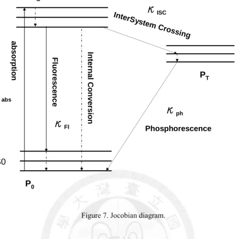
There is generally a triplet state existing between its singlet excited state and ground state for organic molecules. The transition between the singlet excited state and triplet state is via weak spin-orbit coupling and termed as “Inter-System Crossing (κISC)”. The lifetime of the excited electron is at the time scale of ms or even longer, and this radiative relaxation process generally gives rise to phosphorescence (κph), Figure 7. The existence of triplet state often accelerates photo-bleaching of organic dyes, and leads to intermittence (on-off blinking) behaviour for single-molecule studies.

S1

S0

T1

absorption Fluorescence Internal Conversion

InterSystem

Crossing

Phosphorescence P_S

P₀

P_T

κ

_ISC

κ

_ph

κ

_Fl

κ

_abs

Figure 7. Jocobian diagram.

For autocorrelation of fluorescence intensity, this intersystem crossing results into the bunching effect following the anti-bunching dip [32]. Assume that the population density in ground state is P0 and population densities in singlet excited and triplet state are PS and PT respectively. The absorption, fluorescence, intersystem-crossing and phosphorescence rate are termed as

κ

abs

, κ

FI

, κ

ISC and

κ

phindividually, Figure 7. In equilibrium, the population densities of the three states are dependent on one another, Equation (32).

) 1 (

; ) 1

0

(

T

abs FI

abx S

T abs

FI

FI

P P P

P ⋅ −

= +

− + ⋅

= κ κ

κ κ

κ κ

(32)

The solution to the rate equation of this three-level system is described by Equation (33) (stimulated emission is assumed absent in low excitation rate). The convolution of exponential function still takes the same mathematical form, Equation (34), but the prefactor varies.

abs FI

ISC abs

ph t

S

a b e

P κ κ

κ κ κ

λ

λ

+ + ⋅

=

⋅ +

=

⁻

;

(33)

) (

; 1

)

2

(

abs FI

ph

ISC t

c

abx

e c

G κ κ κ

κ

τ

^λ

κ

+

⋅

= ⋅

⋅ +

=

⁻

(34)

The picture concerning the bunching effect is quite straightforward. In the beginning, the molecule is emitting photons at a higher rate, but trapping by the triplet state in the following makes it silent on the order of its triplet lifetime (~ μs – ms). After the molecule return to its ground state, it becomes active and capable of emitting light again until the next trapping [7, 9]. Discussions above stay in the regime of low excitation rate. The discussion over intensity autocorrelation analysis at high excitation rate (sufficient to initiate stimulated emission) is beyond the scope of the discussion in this chapter.

Anti-bunching of Single Fluorescent Object

To study reactions occurring at shorter time scale (below μs), artefacts from detectors should be taken into account. Real detectors suffer from dead time limitations and afterpulsing effects. Dead time is defined as a period of time in which a detector is “blind”

after detecting an event. In other words, a detector could not receive two events whose spacing is shorter than its dead time. Take avalanche photodiode (APD) as an example, its dead time is around 100 ns. Therefore, if only one detector is in use for autocorrelation analysis, it could never be possible to have the shortest time scale go below its dead time.

2.3.4: Other Sources of Fluorescence Fluctuations

In addition to the triplet state of molecules, there are still some other sources which might give rise to bunching effect [7, 9]. The first one is often seen at low temperature [33], and it is attributed to the sharp absorption lineshape and excitation with a narrow-banded laser.

Variations in the absorption spectrum of the molecule could lead to intensity fluctuations since the molecule might be out of the excitation resonance from time to time. Beside the

moment with respect to the polarization of excitation will also come into play [34].

“Blinking” is an important feature of immobilized single molecule behaviour. However, its origins are still not clear and quite complicated [35]. For organic dyes, the origin of on- off blinking is generally attributed to the triplet state. Nevertheless, there are still some other factors could dominate the shorter time scale blinking behaviour, especially the addition of a variety of chemicals to prevent photobleaching [36-38]. The source of the blinking behaviour of quantum dots is quite different from that of organic dyes. Since the electron is created by excitation in the outer shell of a quantum dot, the loss of that electron will prevent the electron-hole from recombining such that the quantum dot is like being trapped in a dark state. Photobleaching is the last source people would like to see in the autocorrelation experiment for its confusion with other sources in study.

CHAPTER 3

APPLICATIONS OF CORRELATION ANALYSIS

The results and discussions in chapter 3 are based on fluorescence intensity analysis.

Nevertheless, a lot of factors could bias the results of intensity analysis, such as scattered light and background photons [39]. Correlation analysis on the intensity which is sensitive to the signal variations could assist in clarifying the origins of fluorescence fluctuations.

On the other hand, time correlated single photon counting (TCSPC), which records the time difference of each pair of detected photons or arrival time of a photon relative to the trigger precisely, provides us with further information pertinent to either fluorescence lifetime or correlation analysis at short time scale (< 1 µsec). In this chapter, our efforts on FCS and TCSPC and their applications are summarized.

3.1: Size Characterization of Fluorescence NanoDiamond (FND)

The negatively charged nitrogen-vacancy defect center, (N-V)^–, in type Ib diamond is a robust fluorescent nano-object which has ultrahigh photo-stability (neither photobleaching nor blinking), and has drawn much attention in recent years [40]. These desirable optical properties, along with its non-toxic nature, have made FND a promising candidate for the applications of bio-imaging [41-43]. Despite the unique photophysical properties of FNDs, the size of this nano-object is an important parameter to characterize since the size- controlled production is not yet well developed. Measurements of FCS on FNDs in free solution can provide the information concerning the average size [44, 45].

sec /

28 . 0 ) 6 (

; 4

2 2

0

D R G m m

D r

D

μ

τ = =

(35)

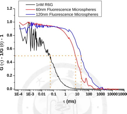
The effective focal volume of the confocal microscope was characterized by the organic dyes, R6G, in advance. Since the diffusivity (diffusion coefficient) of R6G is known (0.28 µm²/msec), the effective focal volume can be obtained by fitting to the 3D-diffusion model, Equation (28). The calibrated dimension of the excitation focal volume is 0.34 µm in r0

diffusing particles affects the fluorescence autocorrelation curves is illustrated in Figure 8.

Fluorescence microspheres with different diameters (60 nm and 120 nm) are measured and compared with R6G. The fluorescence autocorrelation curve shifts to the longer time scale (right-handed side) as the particle size increases.

1E-4 1E-3 0.01 0.1 1 10 100 1000 10000100000 0.0

0.2 0.4 0.6 0.8 1.0 1.2

G

(

τ

)

- 1/G

(

0

)

- 1

τ (ms)

1nM R6G

60nm Fluorescence Microspheres 120nm Fluorescence Microspheres

Figure 8. Normalized auto-correlation curves of organic dyes (R6G), 60 nm and 120 nm fluorescence microspheres. The effective focal volume of the confocal microscope is characterized by the organic dyes, R6G, and its diffusion coefficient is 0.28 µm²/msec.

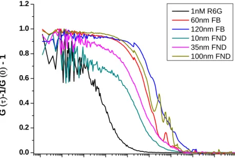
Three different sized FNDs (10 nm, 35 nm and 100 nm) in free solution are measured, Figure 9. Fluorescence microspheres (60 nm and 120 nm) serves as references, and the shape effects are neglected [46].

1E-4 1E-3 0.01 0.1 1 10 100 1000 10000100000 0.0

0.2 0.4 0.6 0.8 1.0 1.2

G

(

τ

)

-1/G

(

0

)

- 1

τ(ms)

1nM R6G 60nm FB 120nm FB 10nm FND 35nm FND 100nm FND

Figure 9. Comparison of the autocorrelation curves of different-sized FNDs and fluorescence micro-spheres in FCS

3.2: Determination of Flow velocity of Microfluidic Mixer

The advantage of micro-fluidic mixer based on “hydrodynamic focusing” is the potential to achieve sub-ms mixing dead time (~ 10 µs) and low sample consumption rate [47-51].

The principle of hydrodynamic focusing is that mixing is via diffusion and achieved by reducing the dimension of mixing region. Its applications in the study of kinetics of biomolecules arouse a lot of interests, especially in the research of protein folding.

However, the velocity of flow (or travelling velocity of sample particles) plays an important role in time resolution of this continuous-flow mixing system. The nature of the parabolic flow velocity profile in micro-channels fails the sub-ms mixing dead time under the conventional wide-field imaging system due to the long depth of field. On the other hand, the lack of precise measurements on the velocity in micro-fluidics imposes more uncertainties on the time resolution. Confocal microscopy combining with correlation analysis is one of the solutions to this problem.

26 26

Inlet : 60nm FB Side : DI water

60 nm FB

DI water

Figure 10. Schematic illustration of the optical system (confocal microscopy with FCS) [52]

This work is collaborated with Dr. Chien-Cheng Chang and Dr. Chin-Chou Chu in Institute of Applied Mechanics, National Taiwan University. They are responsible for simulations on momentum/mass transportation and fabrications of microfluidic mixing devices [52]. Figure 10 shows the schematic representation of the data acquisition system based on confocal microscopy and FCS. Our home-built confocal microscope can be switched to the wide-field mode to locate the cross regime of the mixer (left panel, Figure 10); the picture was taken by a charge coupling device (EMCCD 887-BUV, Andor Technology). Three inlet flows are driven by syringe pumps, and the flow rates are manually adjusted. The whole device is mounted onto the peizo-stage, and stage-scanning mode is used for confocal imagining. Fluorescence emission was detected by a photon counting module (APD, avalanche photo-diode, SPCM-AQR- 15-FC, PerkinElmar); the output TTL signals from APD were split into two channels and sent to the data acquisition card and the correlator (ALV-5000, ALV GmbH, Germany) respectively.

17

50 100 150 200 250 300 350 400

50

100

150

200

250

300

350

400

0 136.5 273.0 409.5 546.0 682.5 819.0 955.5 1092 1205

I 2 ul/min : 2 ul/min

50 100 150 200 250 300 350 400

50

100

150

200

250

300

350

400

0 136.5 273.0 409.5 546.0 682.5 819.0 955.5 1092 1205

I 2 ul/min : 4 ul/min

50 100 150 200 250 300 350 400

50

100

150

200

250

300

350

400

0 136.5 273.0 409.5 546.0 682.5 819.0 955.5 1092 1205

I 2 ul/min : 6 ul/min

50 100 150 200 250 300 350 400

50

100

150

200

250

300

350

400

0 130.8 261.7 392.5 523.4 654.2 785.0 915.9 1047 1155

I 2 ul/min : 8 ul/min

50 100 150 200 250 300 350 400

50

100

150

200

250

300

350

400

0 130.3 260.5 390.8 521.1 651.4 781.6 911.9 1042 1150

I 2 ul/min : 10 ul/min

50 100 150 200 250 300 350 400

50

100

150

200

250

300

350

400

0 121.2 242.4 363.6 484.8 606.1 727.3 848.5 969.7 1070

I 2 ul/min : 12 ul/min

Figure 11. Demonstration of hydrodynamics focusing by 60 nm fluorescence microspheres [52]. The central flow carrying microspheres is squeezed by two side flows. The focusing width is decreasing with rising side flow rate.

Fluorescence microspheres (~ 60 nm in diameter) were injected into the microfluidic mixing device from the central inlet to demonstrate hydrodynamic focusing. Two side channels were loaded with DI water. Figure 11 is a series of confocal images with increasing flow rates of side channels. The higher the flow rates of side channels, the tighter the focused central flow which carried fluorescence microspheres. The focusing width was related to the derived mixing dead time; the relation between focusing width and side flow rate is plot in Figure 12.

50 100 150 200 250 300 350 400

50

100

150

200

250

300

350

400

0 136.5 273.0 409.5 546.0 682.5 819.0 955.5 1092 1205

I

2 ul/min : 6 ul/min

Main : Side (ul/min)

W_F(um)

2 : 2 2.3

2 : 4 2.2

2 : 6 0.60

2 : 7 0.64

2 : 8 0.60

2 :10 0.59

2 :12 0.65

0 10 20 30 40

0 200 400 600 800 1000

Intensity(100Hz)

pixel (1pixel=0.1um)

I - 2ul/min : 6ul/min outlet

0 1 2 3 4 5 6 7

0.5 1.0 1.5 2.0 2.5

Wf (um)

Qs/Qi (Qi=2 ul/min)

@4um Focusing width_I

Figure 12. Determination of the focusing widths of the central flow at various flow rate ratios (FM : FS) [52].

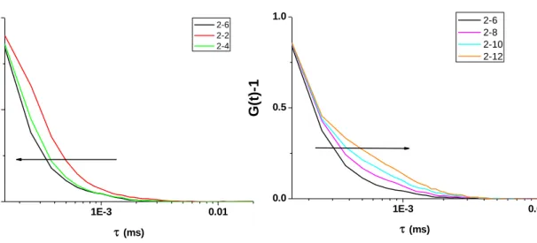
However, the tightest focusing width did not promise the best time resolution since the particle travelling velocity in the squeezed central flow might decrease as the side flow rate goes beyond a certain value (6μl/min in our case) [53], Figure 13. The flow velocity (travelling velocity of the fluorescence microspheres) decreased with the increasing side channel flow rate, Figure 13 B.