國立臺灣大學工學院化學工程學系 碩士論文
Department of Chemical Engineering College of Engineering
National Taiwan University Master Thesis
利用分子動力學模擬探討水合物晶體界面特性 Interfacial Properties of Methane Hydrate and Water via
Molecular Dynamics Simulations
何垚煌 Yao-Huang Ho
指導教授:林祥泰 博士 Advisor: Shiang-Tai Lin, Ph.D.
中華民國 108 年 7 月
July, 2019
致謝
感謝林祥泰老師。在我懵懂無知時,細心的指導我。從不直接告訴我答案,
而是耐心引導,讓我自己想出解決辦法。另外,感謝老師認真聆聽我的意見,
提供我一些工作選擇上的訊息與訊息,讓我明白除了工程師之外的道路。
感謝 David Wu 老師,在這兩年期間,於研究方面給予我很多的指導。
感謝旻聰學長帶我進入分子模擬的世界。學長的教學方法,當年的我覺得 根本是放牛吃草,總是提個開頭,後面就要自己去想辦法解決。與其說學長教 導我分子模擬的知識,倒不如是教導我如何使用 GOOGLE 去找到問題的答案。
但對於現在的我來說,卻是萬分感謝。當我成為其他人的學長時,由於覺得當 年的我學得太痛苦,所以就直接把所有我會的東西交給弟弟們,但後來才發現 他們做了一年甚至快二年了,還常常會問我一些入門級問題,這時才對於學長 的教學方法感觸良深。
感謝姿妤,與我一起在旻聰的教學下一同奮鬥的夥伴。很感謝我的碩士生 涯有妳的相伴。由於我們進實驗室時,做 MD 的學長們都離開了,所有的東 西都是我們兩個重新整理與自己摸索學習的。如果沒有妳我應該會崩潰。想當 初我們連 qsub 後連去哪裡找 job 都不知道,還是依靠你偷偷看老師的指令才 明白 qstat 的存在。
感謝昌哲。在我碩一時,一起陪我玩恰恰谷,與我分享很多生活點滴,以 及時常在我研究有困難時與大仔一起給予我建議。
感謝 Billy。在我碩一還不太會寫 C++時,常常陪我到晚上 11 點,教導我 寫程式,真的很感激你。
感謝子芳、軒豪、德謙、大仔、CCK,陪伴我二年的碩士生涯,從頭至尾。
感謝政廷、柏偉,在我碩二時,讓我遇見了你們,我很高興認識你們。
感謝曉丰、浩恩、藍天三個有點瘋瘋癲癲但都很厲害的專題生。你們帶給 我很多歡笑與神奇小知識。
感謝亞叡、俊霖、大力行、威霖、旻賢與雲杰學長們在我碩零時給我的幫 助。
感謝我父母提供我金錢上的補助,讓我不須煩惱金錢,將心思都放在做研
究上,以及在我研究做不出來時,給我加油打氣,真的非常感激。
感謝我自己。這兩年當中,我其實一度想要放棄研究,因為一直做不出東 西,覺得自己很沒用。但我還是堅持了下來,碩二的 11 月,終於開始做出了 一些成果。我忍受了 18 個月的艱難,最後還是小有成功,把這個研究題目做 完。在這過程中,常常會思考著我想要的人生究竟是甚麼樣子。雖然這 18 個 月過得很痛苦,但也因為如此,更加明白自己未來不想做什麼,以及想做甚麼 事。感謝上帝的安排。
中文摘要
分子動態模擬被用來進行研究冰-h 以及甲烷水合物晶體的表面性質。我們特 別關注於其熱力學性質以及表面波動的動態性質。根據毛細管波動理論,我們測量 出對於冰-h 在 270K 以及甲烷水合物在 285K 下,其界面自由能各為 29.24 與 34.60
mJ/m2。這個結果與實驗值非常相似。在實驗中,冰-h 在 250K 至 283K 下其界面
自由能為 25 至 35mJ/m2;而甲烷水合物則是在 260K 至 285K 下,其介面能為 31
至 36mJ/m2。我們的模擬表明,晶體面相對於界面自由能的影響很小,冰-h 和甲
烷水合物分別只有 1%和 3%。隨著冰-h 和甲烷水合物晶體的波長增加,表面波的 弛豫會漸漸地被毛細波支配。此外,在液相擴散的時間尺度特徵中,甲烷水合物晶 體的弛豫時間幾乎是冰-h-晶體的 40 倍。我們將這種差異歸因於復雜的氫鍵生成與 斷裂和籠狀結構的水合物的存在。最後,我們通過模擬毛細波動力學來估計動力係
數(晶體生長速率取決於過冷度),並將冰-h 和甲烷水合物晶體的動力係數與之前
的模擬值與實驗值做比較
關鍵字:表面波動、界面自由能、晶體面相、熱力學、動力學、分子動力學模擬
ABSTRACT
Molecular dynamics (MD) simulations were conducted to study the crystal-melt interface of ice and sI methane hydrate crystals. In particular, we focus on both the thermodynamics and dynamics of surface waves. Based on the capillary fluctuation theory, we determined the interfacial free energy of Ice-H (Ih)/water and sI methane hydrate/water to be 29.24mN/m2 at 270K and slightly higher value, 34.60 mN/m2 at 285K, respectively. The results are consistent with experiment, 25~35 mJ/m2 at 250K to 283K for Ih/water interface, and 31~36 mJ/m2 at 260K to 285K, for the sI methane hydrate/water interface. Our simulations show that the effect of orientation of crystal to interfacial free energy is small, only 1% and 3% for Ih/water and sI methane hydrate/water, respectively.
The relaxation of surface waves are dominated by the slow process as the wavelength increases for both Ih and sI methane hydrate crystal. Moreover, in a time scale characteristic for the diffusion of the liquid phase, the relaxation time of the crystal-melt interface of sI methane hydrate crystal is almost 40 times slower than that of Ih crystal.
We ascribe this difference to the presence of complicate hydrogen bond network and cage-like configuration of hydrate. Finally, we estimate the kinetic coefficient (rate of crystal growth depends the degree of supercooling) from our simulation of the capillary wave dynamics and compare it with previous simulation studies and with experiments for the case of Ih and sI methane hydrate crystal.
Keywords: Surface Wave; Interfacial Free Energy; Crystal Orientation;
Thermodynamics; Dynamics; Simulation.
致謝 ... 1
中文摘要 ... 3
ABSTRACT ... 4
LIST OF FIGURES ... 8
LIST OF TABLES ... 14
Chapter 1 Clathrate Hydrates ... 16
1.1 Clathrate Hydrates ... 16
1.2 Application of Clathrate Hydrates ... 18
1.3 Surface fluctuation of the interface of solid/fluid ... 21
1.4 Sodium Dodecyl Sulfate ... 23
1.5 Motivations... 24
Chapter 2 Theory ... 27
2.1 Molecular Dynamics Simulation ... 27
2.2 Integration of Equation of Motion ... 29
2.3 Force field ... 29
2.3.1 Non-Bond Terms ... 30
2.3.2 Valence Terms ... 32
2.4 Ensemble ... 33
2.5 Temperature Thermostat ... 33
2.6 Pressure Barostat ... 34
2.7 MSD (mean square displacement) ... 35
2.8 ACF (autocorrelation function) ... 35
2.9 Physical meaning for some interfacial technical terms... 36
2.9.1 Surface stress ... 36
2.9.3 Stiffness ... 37
2.10 Calculation of surface stress from MD simulation ... 37
2.11 Mold integration method ... 38
2.12 F4 order parameter ... 40
2.13 Capillary Fluctuation Theory ... 40
Chapter 3 Computational Details... 45
3.1 Models ... 45
3.1.1 Models for melting point of sI CH4 hydrate & Ih ... 46
3.1.2 Models for diffusivity of H2O at different melting condition ... 47
3.1.3 Models for heat of fusion of Ih & sI methane hydrate ... 48
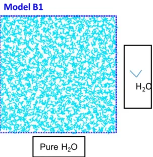
3.1.4 Models for mold integration method of H2O system ... 49
3.1.5 Models for capillary fluctuation method of Ih/water ... 50
3.1.6 Models for capillary fluctuation of sI methane hydrate/water .... 52
3.1.7 Models for capillary fluctuation of SDS/methane hydrate/water 53 3.2 The setting of temperature and pressure condition ... 54
3.3 Method to generate the solid/liquid coexistence system ... 55
3.4 Force Field... 56
3.5 Hydrogen Bond Identification ... 57
3.6 Position of Interface Solid/Fluid System Identification... 58
Chapter 4 Results and Discussion ... 60
4.1 Properties of CH4 hydrate and Ih ... 60
4.1.1 Bulk Phase Properties of CH4 hydrate and Ih ... 60
4.2 Interfacial Properties of Methane Hydrate and Water ... 63
4.2.1 The performance of F4 order parameter ... 64
4.2.3 Thermodynamics properties of CMI system of CH4 hydrate ... 71
4.2.4 Thermodynamics properties of CMI system with SDS of CH4 hydrate ... 73
4.2.5 The validation by Mold Integration method ... 75
4.2.6 Dynamics properties of CMI system of Ih ... 80
4.2.7 Dynamics properties of CMI system of CH4 hydrate ... 87
4.2.8 Effect of parameters to CMI ... 97
Chapter 5 Conclusions ... 100
References ... 103
LIST OF FIGURES
Figure 1.1-1 Different types of cages: pentagonal dodecahedron (512), tetrakaidecahedron (51262), hexakaidecahedra (51264), dodecahedron (435663), icosahedron (51268).
Different cages with specific ratio can constitute structure I, structure II and
structure H [4]... 17
Figure 1.2-1 Distribution of gas hydrate around the world [12]. ... 19
Figure 1.2-2 Phase diagram of hydrates. (pink line: equilibrium line of CH4 hydrates from experiments; green line: equilibrium line of CO2 hydrates from experiments; gray line: vapor- liquid equilibrium line of pure CO2 [12]. ... 20
Figure 1.4-1 Structure of the SDS ... 23
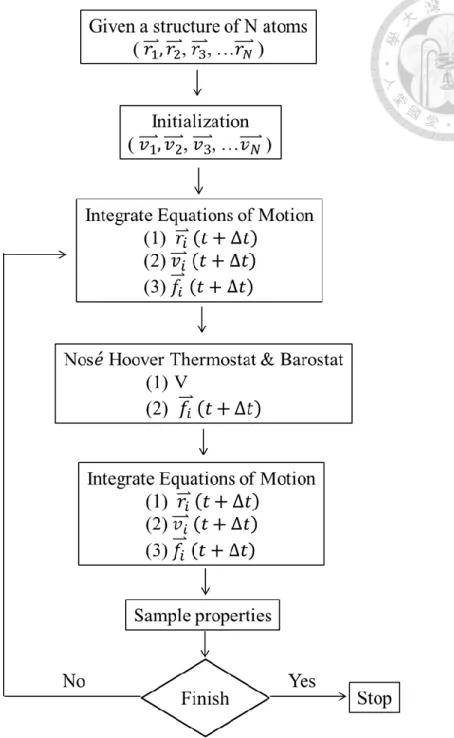
Figure 2.1-1 The flowchart of MD simulation. ... 28
Figure 2.3-1 The component of Ewald summation[78]. ... 32
Figure 2.12-1 Illustration of criteria of F4 calculation... 40
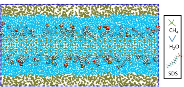
Figure 2.13-1 Snapshot of a typical configuration for capillary wave simulation. Only represents oxygen atom of H2O. Particles colored by red denotes fluid-like, colored by white if they have crystalline behavior, and colored by blue represents the interface position. The symbols 𝑣 , 𝑠 𝑎𝑛𝑑 𝑛 represent wave prorogation direction, the shortest depth length direction, and normal vector direction of CMI, respectively. Lv, Ls. and Ln denotes the length of simulation box along with 𝑣 , 𝑠 𝑎𝑛𝑑 𝑛, respectively. ... 41
Figure 2.13-2 Illustration the h(vn,t) and . Snapshot of a configuration of a hydrate slab in equilibrium with liquid water, and the color symbols are as same as Figure3. ... 43
Figure 3.1-2 Models for melting point of CH4 hydrate crystal. ... 47
Figure 3.1-3 Models for diffusivity of fluid-like H2O at melting condition of Ih and CH4 hydrate ... 48
Figure 3.1-4 Models for heat of fusion of Ih hydrate. ... 49
Figure 3.1-5 Models for heat of fusion of CH4 hydrate. ... 49
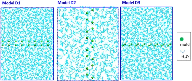
Figure 3.1-6 Models for mold integration of pI (D1), pII (D2) and basal (D3) plane of Ih/water. The snapshots of all Figures are viewed from side of normal direction of interface. ... 50
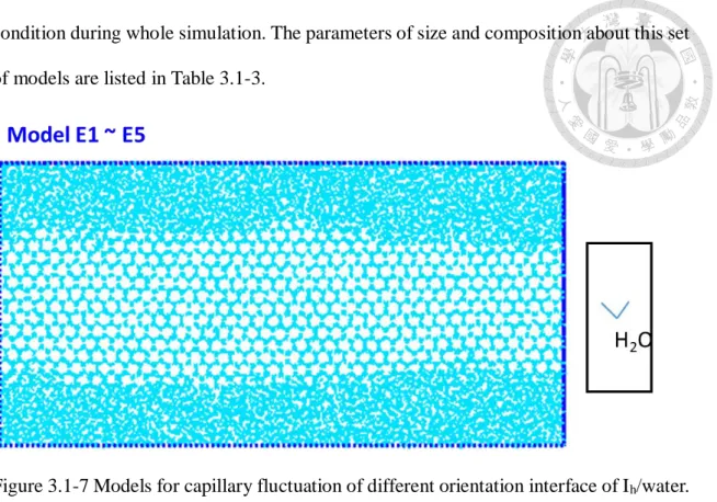
Figure 3.1-7 Models for capillary fluctuation of different orientation interface of Ih/water. ... 51
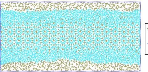
Figure 3.1-8 Models for capillary fluctuation of different orientation interface of methane hydrate/water ... 52
Figure 3.1-9 Models for capillary fluctuation of different orientation interface of SDS/methane hydrate/water ... 53
Figure 3.2-1 The flowchart of simulation. ... 55
Figure 3.5-1 Two criteria of identification of hydrogen bond. ... 58
Figure 3.6-1. The schematic of interface position determination. ... 59
Figure 4.1-1 Potential energy of (a) Ih and (b) sI-CH4 hydrate versus different temperature. ... 61
Figure 4.2-1 (a) F4 probability distribution of the system with no block-average. (b) block-average size is set as 4. (c) block-average size is set as 20. (d) block- average size is set as 40. The line colored by azure, orange and silver denote Ih, water, and sI hydrate, respectively. ... 66 Figure 4.2-2 Plots of ln[ <|hq|2>A/kBT ] versus ln(q) for all Ih/water with different orientations studies. The unit of <|h |2>A/k T is used in m3*N-1 and q is given
in m-1. The red solid-lines shown in (a) ~ (e) are linear fits with slope -2 at low-q region. The intercept of the fitting is –ln() , and the unit of calculating by intercept is N/m. ... 69 Figure 4.2-3 Coordinate system of Ih, , are spherical coordinate angles used to define the orientation of normal vector direction (𝑛) to CMI.[109] ... 69 Figure 4.2-4 Plots of ln[ <|hq|2>A/kBT ] versus ln(q) for all sI hydrate/water with different orientations studies. The unit of <|hq|2>A/kBT is used in m3*N-1 and q is given in m-1. The orange solid-lines shown in (a) ~ (c) are linear fits with slope -2 at low-q region. The intercept of the fitting is –ln(). ... 72 Figure 4.2-5 ln[ <|hq|2>A/kBT ] versus ln(q) for [010](100) sI hydrate/water case. The -2 slope is fitted by the data point at the middle frequency region of run 1. ... 75 Figure 4.2-6 The F4 of the system at different rw conditions. ... 76 Figure 4.2-7 Average number of filled wells versus well depth ( ϵ /kBT) for the pII plane of the TIP4P/Ice model. The radius of the mold wells is (a) rw=1.30 Å and (b) 1.25 Å . Orange circles (blue line) correspond to simulations starting from an equilibrated configuration with the mold switched on (off)... 78 Figure 4.2-8 Filled symbols: interfacial free energy for different values of the well radius and crystal orientations of Ih. Orange, blue, and gray denote pII, pI and basal, respectively. Dash lines indicate the linear fits to filled symbols. Points with vertical line indicate row. ... 79 Figure 4.2-9 Filled symbols: interfacial free energy for different values of the well radius of pII plane of Ih. Blue, purple, and green denote 32, 64 and 128 numbers of mold, respectively. ... 79
respectively. ... 82 Figure 4.2-11 The representation of dln (fq(t)/dt vs t for Ih [pI](pII). The color of azure, orange, and silver denote k=1, k=2, and k=3, respectively. ... 82 Figure 4.2-12 Prefactor for the double exponential fit as function of q for water [pII](pI). ... 83 Figure 4.2-13 (a) Dimensionless characteristic time for the slow relaxation process, ds, versus the dimensionless wave-vector q/-1 in a double logarithmic scale for all orientation interface. The orange dash line symbolizes -2 slope linear straight line (ds ∝ q − 2) (b) Dimensionless characteristic time for the fast relaxation process, df, plotted against the dimensionless wave-vector q/-
1. ... 84 Figure 4.2-14 ds∗ q2 in logarithmic scale versus against with q. Azure, orange, silver, yellow, and blue denote [pI](basal), [basal](pI), [pII[](pI), [basal](pII) and [pI](pII), respectively. ... 85 Figure 4.2-15 Crystal growth rate as a function of degree of subcooling (T). Yellow line denotes experimental result by Pruppacher[116]. Blue line indicates simulation result by Rozmanov[117]. Brown line is the result by this work. ... 86 Figure 4.2-16 (a) Autocorrelation functions for the sI hydrate [010](100). (b) [110](110) (c) [110](100) ... 88 Figure 4.2-17 Prefactor for the double exponential fit as function of q for sI hydrate. The line color by azure, silver and orange is represented by [010](100), [110](- 110) and [110](100), respectively ... 89 Figure 4.2-18 (a) Dimensionless characteristic time for the slow relaxation process, ds,
versus the dimensionless wave-vector q/-1 in a double logarithmic scale for all orientation interface. The green dash line symbolizes -2 slope linear straight line (ds ∝ q − 2) (b) Dimensionless characteristic time for the fast relaxation process, df, plotted against the dimensionless wave-vector q/-1.
The line color are shown in azure, silver and orange symbolized as [010](100), [110](-110) and [110](100), respectively. ... 91 Figure 4.2-19 ds∗ q2 in logarithmic scale versus against with q. Azure, orange, and silver denote [010](100), [110](110), and [110](100), respectively. ... 92 Figure 4.2-20 Crystal growth rate as a function of degree of subcooling (T). Orange line denotes experimental result by C.J.Taylor[118]. Yellow line indicates simulation result by JY,Wu [102]. Azure and silver line are the results done by this work. ... 92 Figure 4.2-21 Crystal growth rate as a function of degree of subcooling (T). The heavy-
blue curve is plotted by the method as same as JY,Wu [102] but in multiple temperature condition. ... 94 Figure 4.2-22 Motion of CH4 atom during the simulation. Green and red denote the methane atoms initially located at the interface and gas phase, respectively.
(a) t=0. (b) 42ns. (c) 84ns ... 95 Figure 4.2-23 The CH4 concentration in each of the layers compares with different orientation to CMI. Width of each of the layers is 4.125A which is the average of the radius of small cage and big cage of sI-hydrate. Layer 0 symbolizes the first layer under the CMI. Layer 1, 2, 3, and 4 denote 1st, 2nd, 3rd, and 4th layer over the CMI, respectively. ... 96
layer... 96 Figure 4.2-25 The effect of block size to the CMI ... 98 Figure 4.2-26 The effect of number of discrete points to the CMI (a) [110](-110). (b) [110](100). (c) [010](100). ... 99
LIST OF TABLES
Table 1.1-1 Geometry of cages in different hydrate structure [5]. ... 17
Table 3.1-1 The composition and simulation targets of model A1~G3. ... 45
Table 3.1-2 System size and composition for the models of mold integration ... 50
Table 3.1-3 The system size and composition for the models of capillary fluctuation for Ih/water system. The Miller index in the square bracket and parenthesis indicate the direction parallel to the direction of propagation of surface wave, and the direction parallel to the normal of the interface, respectively. ... 51
Table 3.1-4 The system size and composition for the models of capillary fluctuation for methane hydrate/water system. ... 52
Table 3.1-5 The system size and composition for the models of capillary fluctuation for methane hydrate/water system. ... 54
Table 3.2-1. The composition and simulation targets of model A1~A2, B1~B2, C1~C4, D1~D3, E1~E5, F1~F3 and G1~G3 ... 55
Table 3.4-1 Parameters used in this work: (a) Van der Waals and Coulomb (b) modified cross term (c) bond (d) angle ... 56
Table 4.1-1 Overall work on detecting the melting point of Ih and sI CH4 hydrate ... 62
Table 4.1-2 Overall work about diffusivity (unit: cm2/s) of H2O at various melting-point condition ... 62
Table 4.1-3 Fusion heat of Ih and sI CH4 hydrate at melting-point condition ... 62
Table 4.2-1 the interfacial stiffness (unit: mN/m) of each orientation for Ih/Water. ... 69
Table 4.2-2 The expression of normalized spherical harmonics function [108] ... 69 Table 4.2-3 Interfacial free energy in terms of normalized spherical harmonics for
Table 4.2-4 Stiffness in terms of normalized spherical harmonics for different orientations ... 70 Table 4.2-5 Interfacial free energy of different orientation of Ih ... 71 Table 4.2-6 The stiffness and expression of cubic harmonics function for different orientations ... 73 Table 4.2-7 Comparison of interfacial free energy of methane hydrate and water with experiment ... 73 Table 4.2-8 Summarize the r𝑤o and interfacial energy of basal, pI, and pII plane. ... 76 Table 4.2-9 Comparing the interfacial energy of basal, pI, and pII plane by MI and CFT in this work. ... 76 Table 4.2-10 Overall simulation work about interfacial free energy of Ih/water (unit:
mN/m). MI, CMS, CNT, and CFT are corresponded to Mold-integration, Cleaving-methods, Classical-nucleation theory, and Capillary-fluctuation theory, respectively. The value of interfacial tension of MI, CMs, CNT, and CFT is obtained from ref. [31, 43, 45, 47], respectively. The * mark denotes the result verified by this work. ... 80 Table 4.2-11 Kinetic coefficient for different orientations of Ih/water ... 86 Table 4.2-12 Kinetic coefficient for different orientations of sI CH4-hydrate/water ... 93
Chapter 1 Clathrate Hydrates
1.1 Clathrate Hydrates
From a macroscopic view, clathrate hydrates are a kind of non-stoichiometric crystal solid, in which guest molecules such as methane (CH4), carbon dioxide (CO2) or hydrogen can be trapped. CH4 hydrate can naturally nucleate and grow under the environment of low temperatures and high pressures, like permafrost regions or the deep seafloor below the ocean. Because there are a great amount of methane gas trapped in the hydrate all over the world [1-3], it has been considered as a new potential source of energy
From a microcosmic view, gas hydrate is consisted of gas molecules, usually called guest molecules, are enclathrated by the rigid water cage via hydrogen bonds. The water cage is constructed by polygon rings, for example, the dodecahedron (512) is composed of twelve pentagons, and the tetrakaidecahedron (51262) is composed of twelve pentagons and two hexagons. Using different cages with specific ratio can constitute different types of structure of hydrate, the most common structures of hydrate are structure I (sI), structure two (sII) and structure H (sH), as shown in Figure 1.1-1. For instance, a unit cell of the sI hydrate is composed of two 512 (small) cages and six 51262 (large) cages.
According to the thermodynamics stability, pentagons and tetrakaidecahedron can trap one guest gas, so there are 8 guests in a unit cell of sI under full-occupied cages condition.
Due to the size of guest molecules and the geometry of cages listed in Table 1.1-1, different kinds of guest will form specific hydrate structure which the thermodynamics property is the most stable. For example, the size of guest molecules between 4.2 Å and 6 Å , such as methane, ethane and carbon dioxide, can usually form sI and sII hydrate
In this work, we only discuss both the thermodynamics and dynamics properties for sI CH4 hydrate structure under the liquid/solid coexistence condition.
Figure 1.1-1 Different types of cages: pentagonal dodecahedron (512), tetrakaidecahedron (51262), hexakaidecahedra (51264), dodecahedron (435663), icosahedron (51268). Different cages with specific ratio can constitute structure I, structure II and structure H [4].
Table 1.1-1 Geometry of cages in different hydrate structure [5].
structure I II H
Cavity small large small large small medium large
Name 512 51262 512 51262 512 435663 51268
No. of cavities/ unit cell 2 6 16 8 3 2 1
Average in radius (Å ) 3.95 4.33 3.91 4.73 3.94 4.04 5.79 Variation in radius (%) 3.4 14.4 5.5 1.73 4.0 8.5 15.1 No. of water molecules
/cavity
20 24 20 28 20 20 36
1.2 Application of Clathrate Hydrates
Gas hydrates have been first paid an attention in petroleum industry, because the temperature and pressure of the transporting-petroleum pipeline is in thermodynamics stable region of formation the nature gas hydrates resulting in the blockage of pipelines.
[6-8]. However, in recent years, other applications of hydrate, such as gas transportation or direct energy source of methane gas attract much attention.
Although there are lots of different kinds of clathrate hydrates, the CH4 hydrates are the most common one, which been found in permafrost and sea floors. The amount of methane enclathrated in hydrate and distribute whole the world, so that it is regarded as a new potential energy source [3, 9-11]. The distribution of CH4 hydrate [12] is shown in Figure 1.1-1. The storage capability of methane in hydrate distributed whole the world is estimated to be around ~3×10¹³ m3 [13], which is almost sane as the shale gas deposits in the USA [14]. Therefore, finding out feasible methods to exploit the methane from CH4
hydrate is unstoppable, especially for Taiwan. In Taiwan, except for the great amount of CH4 hydrate [15] discovered under the southwestern offshore Taiwan, there is nearly not found oil, shale gas or any other raw materials. Because of above reason, gas hydrate can become an important energy source for Taiwan.
In addition to being an energy material, hydrate can also be used as a medium of gas transportation. By boxing the gas molecules into the cages, such as natural gas [6, 16], CO2 [6] and H2 [17-21], comparing to traditional LNG method, the gas can be transported under a higher temperatures and lower pressures by a solid crystal form directly. Within certain distance, it’s the most economical method of gas transportation [22].
In this few years, the issue about environment, such as the emissions of CO2 and
methane hydrates spread all over the world, exploiting these resources from the seafloors is concerned by the possibility of forming the tsunami. Furthermore, if the exploited CH4
leaks into the atmosphere, the degree of global warming caused by CH4 is more serious than CO2. In recent years, some scientists propose a new method, called CO2 sequestration, to overcome the problem of greenhouse gas and extracting CH4 from the hydrates at the meanwhile. According to phase diagram shown in Figure 1.2-2, it is possible to recover the CH4 gas from the hydrate and entrap the CO2 into the cavity of the cage of the original methane hydrate. This method can achieve three goal simultaneously. First, extract the energy resource, methane gas, from the methane hydrate on the seafloors. Seconds, reducing the emissions of CO2 in the atmosphere retards the global warming. Third, without melting the hydrate in the seafloors, there is not any possibility of occurring tsunami. [23].
Figure 1.2-1 Distribution of gas hydrate around the world [12].
Figure 1.2-2 Phase diagram of hydrates. (pink line: equilibrium line of CH4 hydrates from experiments; green line: equilibrium line of CO2 hydrates from experiments; gray line:
vapor- liquid equilibrium line of pure CO2 [12].
0 2 4 6 8 10 12 14
270 275 280 285 290 295
P (M P a )
T (K)
CH4 hydrates (experiment) CO2 hydrates (experiment) pure CO2 VLE
CH4hydrate dissociation CO2hydrate dissociation CH4hydrate growth
CO2hydrate growth CH4hydrate dissociation CO2hydrate growth
1.3 Surface fluctuation of the interface of solid/fluid
The interfacial properties (e.g., stiffness, surface tension) of a crystal-melt interface (CMI) have a great influence on the nucleation and growth of the crystal [24-26].
However, the CMI is far less understood than fluid-fluid interface because the measurements involving CMI are much more challenging with typical experimental instrument and method. It is well accepted that the interfacial free energy between the water and air at normal condition is 72mN/m; however, there is a great discrepancy in the reported interfacial free energy between ice and water at ambient pressure, ranging from 25 to 35mN/m [27-30] The analysis of CMI dynamics is useful for understanding the crystal-growth properties [31]
The CMI interface is not static but undulates due to thermal fluctuations. For length scales below the capillary length, the surface wave (SW) is mainly dominated by the interfacial stiffness known as capillary waves (CW). The equilibrium thermodynamic and dynamics properties of CW at the fluid-fluid interface were studied by Smoluchowski and Kelvin [32]. For the CMI, the study of the CW spectrum provides static properties, like the interfacial stiffness and also the interfacial free energy [31, 33-36].
At smaller length scales and higher frequency, the surface of elastic media exhibits thermal vibration known as the name of Rayleigh wave [37]. These waves are small amplitude but high frequency vibrations that result from the elastic response of the solid. The solid phase is elastic and principally exhibit Rayleigh waves. On the other hands, the fluid phase is viscous and would rather show capillary wave.
Unfortunately, although there are fair amount of theoretical researches in this field, it seems like there is not an appropriate theory can fully describe the CMI dynamics through Rayleigh wave or Kelvin wave theory [38-41]. In 1993, Karma published a theory
for the relaxation dynamics of crystal-melt CW based on a diffusion equation of the interfacial profile [33]. The theory shows there exist a power law relationship between a characteristic relaxation time and reciprocal space vector. According to this reason, there were fair amount simulations focused on CMI system and showed that at lower reciprocal space vector region, the simulation results agreed with the Karma’s theory [31, 34-36, 42]
and the interfacial stiffness and interfacial free energy, by means of an analysis of the spectrum of interface fluctuations, calculated by Karma’s theory can reproduce the experiment results [36]. Although, there are existing other computational methods to calculate the crystal-fluid interfacial free energy: the cleaving method[43, 44], classical nucleation theory method[45] and mold integration method.[46, 47], it seems like these methods cannot measure the dynamic properties and other interracial properties.
1.4 Sodium Dodecyl Sulfate
Sodium Dodecyl Sulfate (SDS) is a kind of famous surfactant which is composed of hydrophilic head group and hydrophobic tail.
In the 1990s, Kalogerakis et al. first reported that the rate of methane hydrate formation could be enhanced by adding SDS.[48]
Okutani et al. later discovered that methane hydrate formed in the unstirred chamber with existing SDS not only can promote the nucleation rate but also worked better than other kinds of surfactant (sodium tetradecyl sulfate, hexadecyl sulfate).[49]
Beside, Yoslim et al. found that in the nucleation process, hydrates do not form as a thin solid layer on the gas/liquid interface without surfactant, however, if adding SDS, the nucleation will occur at the solid(container)/gas/liquid where a three phase intersection place.[50]
Figure 1.4-1 Structure of the SDS
1.5 Motivations
Clathrate hydrates are a kind of nonstoichiometric crystalline compounds consisting of cavities (or cages) formed by hydrogen-bonded water molecules where guest molecules are trapped.[51] The empty lattice (cavities) is thermodynamically unstable, and its existence is stabilized by hydrogen bond resulting from the enclathration of the trapped solutes in its cages. [51] Methane is one kind of guest molecules that stabilizes the water cages in the clathrate hydrate structure. There are three known common hydrate structures: sI, sII and sH. [51] In type I hydrate, methane clathrate hydrates have attracted much attention because the large amount found in nature can be a potential source of energy.[52] However, it is still unknown for the mechanism of hydrate formation (nucleation). There are many efforts made to better understand the nucleation mechanism of gas hydrates. Sloan et al.,[53-56] in order to describe the kinetic data of gas hydrate formation,[57] proposed a hypothetical model based on the labile cluster hypothesis (LCH), where the mixture of guest molecules and labile cages formed by water and then may combine to form a nucleus. Radhakrishnan et al.[58] argued that the high energy barriers of forming larger aggregates from labile clusters should not exist in a nucleation process. They proposed a local structuring hypothesis (LSH), where a group of the guest molecules are arranged in a configuration similar to that in the clathrate phase as a result of thermal fluctuation. When sufficient gas molecules are solved, the arrangement of the gas cluster also helps the surrounding water molecules re-orientate to form a nuclei. The LSH was later supported by the results of molecular dynamics (MD) simulations from Rodger and co-workers.[59] In 2009, Walsh et al.[60] reported the first unconstrained MD simulations of methane hydrate nucleation on the microsecond time scale. They
(512), also proposed the mutually coordinated guests theory (MCG).[61] When the cluster of MCGs size is larger than the critical size, the nuclei will be favorite to grow to clathrate crystalline structure; otherwise, the nuclei will be fluctuate and then disappeared.[62]
Jacobson et al. studied the nucleation process using MD simulations.[63] They observed the constant formation and dissociation of guest-rich amorphous precursors (the morphology of a blob or cylinder) as a result of thermal fluctuation. As the size of the blob (or cylinder) becomes larger than some critical size, the blob can continue to grow and solved in water then transform into crystalline clathrate. Such two-step nucleation, or the blob hypothesis (BH), was also supported by atomistic MD simulations of Vatamanu and Kusalik.[64]
Although there were a lot of paper discussing the phenomenon of nucleation;
however, the paper studied the interfacial free energy, a crucial parameter in nucleation and growth[45, 65, 66], between hydrate crystalline and water can be counted on fingers[67-69] L.C Jacobson et al. calculated the tension by Gibbs-Thomson equation and showed that the tension of amorphous crystal and crystalline are 32 and 36 mJ/m2, respectively.[68] This result is consistent with the experimental results worked by R.
Anderson also using Gibbs-Thomson equation.[67] B.C Knott et al. calculated the interfacial tension by classical nucleation theory, and found that the nucleation rate of homogeneous process is pretty low (310-111 nuclei cm-3s-1). In other words, the homogeneous process is almost impossible reaction path of hydrate nucleation [69]. The curvature of the nuclei in this method theoretically changes during the simulation, but it is treated as constant owing to complication for discussing. Therefore, the value of interfacial energy in this method might not be accurate.
Even if there are handful paper calculating the interfacial free energy between hydrate and water, limited by analysis method, the precision of the interfacial free energy
in other methods comparing to capillary fluctuation theory method is not kind of accuracy and also the further information about hydrate crystalline are not mentioned, for instance, the effect of orientation to hydrate, and kinetic properties. Also, the surfactant, SDS, is verified that can effectively promote the nucleation rate of hydrate forming rate, [48-50] however, the reason that SDS can promote the nucleation rate of CH4 hydrate is still unknown. Though there are some papers claimed that it is caused by the forming SDS micelle,[70-72] but this hypothesis is soon rebelled from several experiments which indicate that SDS would not form the micelle under hydrate forming condition.[73-75]
So far, there is still no any reasonable hypothesis can explain this phenomena. Motivated by these reasons, we use capillary fluctuation method to analyze the CMI between hydrate crystalline and water and also what will be different when SDS adsorb on hydrate interface. In this method, not only the interfacial free energy but also other surface dynamics properties of hydrate crystal can be measured. To get a deeper understanding of the dynamics of the CMI, we analyzed three different systems: ice/water, hydrate/water and SDS/hydrate/water. We show that that relaxation of crystal-melt SW is well described by a double exponential for both two cases. We also show that details of the microscopic dynamics are not important for the relaxation of crystal-melt. Then, we compare the relaxation dynamics of SW for hydrate/water and ice/water with several orientation of CMI. Finally, following the Karma’s theory [33] and several method proposed in [31, 35], we estimate the kinetic coefficient (the constant ratio of crystal growth-rate to degree of supercooling) from our measurements of the CW relaxation dynamics.
Chapter 2 Theory
2.1 Molecular Dynamics Simulation
Molecular dynamics (MD) simulation is a kind of powerful method to study the microscopic dynamics behavior on a molecular level. By MD simulation, we can observe how molecules interact with each other directly, which cannot be easily measure in experiment. Therefore, MD simulation is a very suitable tool to analyze the interface properties between hydrate and water.
MD simulation can calculate the interaction force between atoms based on Newton’s second law of motion at each simulation time. The standard operation process of the MD calculations is shown as Figure 2.1-1. Initially, the position of each atom in the system should be appointed, and the velocity of each atom will be assign by Maxwell-velocity distribution at specific temperature. The position of next moment can be calculated by current position, velocity and Newton’s second law of motion. Since we can calculate the position of each atom in system at every times, in other words, the trajectory of the whole system in a specific time period can be known, so directly observing the microscopic mechanism of molecules is feasible. Furthermore, based on ergodicity, the postulate of statistical mechanics, some macroscopic properties such as total energy of the system or the diffusion coefficient of the molecules can also be obtained by analyzing the enough long ensemble simulation. Comparing the macroscopic results from MD simulation to experiment data, the validity of our simulation can be trusted.
Figure 2.1-1 The flowchart of MD simulation.
2.2 Integration of Equation of Motion
The Leapfrog integrator method is chosen as our MD integrator algorism. [76]. The positions and velocities are updated by atom-interaction force (F (t)) calculated by the positions at time t:
v (t+1
2Δt) =v (t-1
2Δt) +Δt
mF(t) (1)
r(t+Δt)=r(t)+Δtv (t+1
2Δt) (2)
The trajectories generated by Leapfrog are identical to the Verlet algorithm[77], shown as equation (3):
r(t+Δt)=2r(t)-r(t-Δt)+1
mF(t)Δt2+O(Δt4) (3)
The velocity Verlet integrator[77] is one of the other generally used integrator. The equations are listed as equation (4) and (5):
𝐫(t + Δt) = 𝐫(t) + Δt𝐯 +Δt2
m 𝐅(t) (4)
v(t+Δt)=v(t)+Δt
2m[F(t)+F(t+Δt)] (5)
2.3 Force field
The force field refers to the parameter sets of potential model, which are calculated from quantum mechanics and experimental data. The potential energy, between any two atoms in the system, can be calculated by deriving force (according to Newton’s second law) respect to the relative distance of a pair of atoms, shown as the equation (6):
-∂U(t)
∂ri =F(t) (6)
The potential energy of system, U(t) can be contributed into many parts, shown as equation (7):
U=Enon-bond+Evalance=Evdw+Ecoul+Ebond+Eangle+Edihedral (7) The van der Waals interaction (EVDW) and coulomb interaction (Ecoul) are the non- bond terms, which are generated by inducing-interaction in the space. The valance terms, caused by the existence of valance bond, can be departed into bond interaction (Ebond), angle interaction (Eangel) and torsion interaction (Edihedral). The atoms can combine with one or more valance bond(s).
The non-bond interactions are neglected for atoms consisted with 1 or 2 valance bond(s) (the bond and angle interactions). For the atoms combined with more than 4 valance bonds, they are considered as in the different molecules so that only the non-bond interactions are considered. For the atoms combined with 3 valance bond, the torsion interaction, caused from the dihedral-angle of valance bonds, is considered and also equal importance with the non-bond interactions, however, non-bond interaction are combined with a weighting factor in order to avoid non-bond interactions too powerful at this circumstance, and this phenomenon is called 1-4 interaction. In this study, there are only H2O and CH4 molecules, so we only consider about bond, angle interactions and non- bond interaction.
2.3.1 Non-Bond Terms
The van der Waals interaction in the MD simulation describes the repulsive and dispersive interactions. Lennard-Jones 12-6 function is the most popular model to describe the van der Waals in MD simulation, shown as equation (8).
E𝑣𝑑𝑤(𝑟) = 4𝜀[(𝜎
𝑟)12− (𝜎
𝑟)6] (8)
The model is described by two parameters, ɛ is the well depth and σ is the collision diameter. The energy is contributed by two parts: r-6represents attractive term and r-12
treatment for the leading term in Drude model. The r-12 variation is quite reasonable for rare gases, however, it is still too steep for hydrocarbons. Even the above reasons, the Lennard-Jones potential is one of the most common model be used, especially in calculation of large system.
Usually we only define the parameters for pure substance, for example, atom A and B. When we want to consider the non-bond interaction between A and B, the parameters, ɛ AB and σAB will be determined by mixing rule, shown as equation (9) and (10):
ε𝑖𝑗 = √ε𝑖𝑖ε𝑗𝑗 (9)
σ𝑖𝑗 = √σ𝑖𝑖σ𝑗𝑗 (10)
The other type of non-bond parameter is the coulomb interaction, it describes the electrostatic energy of atoms, shown as equation (11):
Ecoul(rij)= qiqj
4πε0rij (11)
However, the coulomb interaction of point charge doesn’t converge in a periodic boundary system since the order of distance-r is -1. To avoid this problem, Ewald et al.
proposed the Ewald summation method[78], commonly applied in computational calculation, it can be efficiently summed the electrostatic interactions between particles in simulation system box or their infinite periodic images. In Ewald sum method, the coulomb interaction is constructed by two parts: short range, which can converge quickly in real space, and long range, which converge quickly in reciprocal space, as Figure 2.3-1.
Figure 2.3-1 The component of Ewald summation[78].
By reorganizing the replica sum the coulomb interaction become:
Ecoul(rij)=1
2∑ ∑ ∑ qiqjerfc(√αrij)
|rij+mL|
Nj=1 Ni=1
∞m + 1
2V∑ ∑ ∑ 4π
k2qiqje-ikrije-(k24α)
Nj=1 Ni=1
k≠0 -α
π
1/2∑Ni=1qi2
(12) It can predict the molecular dynamics motions more accurately with a carful parameterization. Furthermore, according to molecular dynamics motions, we can find out the interaction between atoms in the microscopic level, and observe the mechanism between particles that cannot directly observe in experiment.
2.3.2 Valence Terms
The bond energy describes the chemical bonding interaction between two atoms.
The interaction is imagined as a spring states at the equilibrium length (bond length) l0
and force constant k, shown as equation (13):
Ebond=1
2kl(l-l0)2 (13)
The angle bending energy is also described by a harmonic potential. The various potential energy is contributed to the degree of deviation of angles from their equilibrium values θ , shown as equation (14):
If the molecule is consisted of more than 3 continuous and linear valance bond, the torsion energy, the rotation of chemical bonds from basic plane, is needed to consider.
The value of dihedral energy depends on the difference between dihedral angles and valance bonds, simplified to the following equation:
Edihedral=kϕcos m(ϕ-ϕS) (15)
Where multiplicity m is 1~3. The ϕS is the dihedral angle with the strongest structural energy.
2.4 Ensemble
The concept of ensemble was first introduced into statistical thermodynamics by J.Willard Gibbs[79, 80]. Based on ergodicity, the postulate of statistical thermodynamics, we should analyze a large number of samples to make the simulation results consistent with macroscopic experimental results since not long enough ensemble will be influenced by uncontrollable microscopic details and may lead to different results. There are few different types of ensembles designed to fulfill different macroscopic constraints. For example, isothermal-isobaric ensemble (NPT), system with the same specific pressure and temperature in each sample. Canonical ensemble (NVT) was chosen to simulate the surface fluctuation phenomenon of hydrates at certain volume and temperatures.
2.5 Temperature Thermostat
Nos𝑒́-Hoover temperature thermostat[81] is applied to simulate a heat bath in order to control the temperature of system during whole simulation in this work. An additional external force (Fi) is applied to atoms in the system to maintain the temperature at target value:
Fi=-∂U(ri
' N)
∂ri' +ξmivi (16)
ξ̇=3NQ kB(T-Tset) (17) Where Q is a thermal inertia parameter, reflecting the rate of heat transfer between systems and surrounding heat bath; 𝜉 ̇is a friction factor determined by the difference between real-time temperature (T) and desired temperature (Tset) and Q. N is the number of particles in the simulation box, and kB is the Boltzmann constant.
2.6 Pressure Barostat
In this study, there are two types pressure barostats applied. One pressure controlling we used for our system is Berendsen[82, 83]. The Berendsen barostat rescales the coordinates and box vectors every step, or every nPC steps, with a matrix μ, which has the effect of a first-order kinetic relaxation of the pressure towards a given reference pressure P0 according to equation (18):
dP dt=P0-P
τp (18)
The scaling matrix μ is given by equation (19):
μij=δij-nPCΔt
3τp βij{P0ij-Pij(t)} (19)
where β is the isothermal compressibility of the system. In most cases this will be a diagonal matrix, with equal elements on the diagonal, the value of which is generally not known. It suffices to take a rough estimate because the value of β only influences the non- critical time constant of the pressure relaxation without affecting the average pressure itself, however, it is the most efficient way to scale a box at the beginning of a run.
The other pressure barostat we used is the Parrinello-Rahman barostat[84].
Parrinello-Rahman approach is similar to the Nos𝑒́-Hoover temperature coupling, and gives the true NPT ensemble in theory. By the Parrinello-Rahman barostat, the box
db2
dt2=VW-1b'-1(P-Pref) (20)
Where V is the volume of the simulation box, and W is a matrix parameter that determines the strength of the coupling. The matrices P and Pref are the current and reference pressures, respectively.
Comparing Parrinello-Rahman to Berendsen barostat method, the former controls the system pressure more smoothly and naturally, and the latter one provides a direct pressure controlling, so that there will be a concern for kinetic section. Although there might be a problem for kinetic motions using Berendson, it is a nice choice to quickly let the pressure of system approach to the setting value. After approaching to the target pressure, Parrinello-Rahman is then used to collect the true simulation data.
2.7 MSD (mean square displacement)
To understand whether the guest molecules moved during all nucleation process, to determine the self-diffusion coefficient Da of particles of type A is important, one can use the Einstein relation[85]:
t→∞lim < ‖𝑟𝑖(𝑡) − 𝑟𝑖(0)‖2 >𝑖∈𝐴= 2𝑛𝑡𝐷𝐴 (21) Where 𝑟𝑖(𝑡) is the position of atom i at correlation time t and n is the number of dimension of system. Normally, simulations were hold at 3D space in MD simulation, so n is equal to 3.
2.8 ACF (autocorrelation function)
In the data analysis, sometimes we need to consider the correlation between the data.
The autocorrelation function is a good method that can tell us the relationship between the data. The below line is the definition:
R() =<(𝑋𝑡−)(𝑋2𝑡+−)> (22)
Where is the correlation time, 2 is the variance of whole samples, is the average of all data and X denotes the sample. When R()<0 and R()>0, it means there is negative- correlation and positive-correlation between the specific time-lag () of the data, respectively. When R()=0, it indicates that there is no correlation between the specific time-lag () of the data.
2.9 Physical meaning for some interfacial technical terms
2.9.1 Surface stress
Surface stress () was first defined by Josiah Willard Gibbs as the amount of the
reversible work per unit area needed to elastically stretch an existing surface.
2.9.2 Surface free energy
Surface free energy, which represents the excess free energy per unit area needed to create a new surface. The relation between the surface stress σ, and surface free energy γ, was first pointed out by Shuttleworth [86],
ij = ×𝑖𝑗 + 𝜕
𝜕𝑖𝑗 (23)
where ij is surface stress tensor, is surface free energy, ij is kronecker delta and ij is strain tensor. It is noteworthy that when a liquid/vapor interface is stretched, atoms can move freely to the interface from the bulk. Therefore, the interface can remain its structural and energetic characters, indicating that derivative term in eq. 23 is negligible.
In other words, the surface stress and surface free energy are the same for liquid/vapor system. These two terms have been referred to as the “surface tension.”
However, for solid systems (including solid/vapor or solid/liquid systems), the derivative term cannot be neglected. In this case the surface stress and surface free energy
2.9.3 Stiffness
In the modeling of dendritic solidification the thermal diffusion equation is solved subjected to a boundary condition on the interfacial temperature imposed through a velocity-dependent Gibb–Thomson condition. Specifically, the temperature at any point along the moving crystal–melt interface depends on both curvature (Ri) and normal velocity (Vn) according to the equation:
TL = 𝑇𝑀−𝑇𝑀
𝐿 ∑𝑖=1,2[(𝑛̂) +2(𝑛̂)
`2 ] ∗ 1
𝑅𝑖−𝑉𝑛
(𝑛̂) (24)
where TM is the melting temperature and L the latent heat of melting per unit volume. The second-term on the right-hand side of equation (24) represents the change of the local equilibrium melting point due to the curvature of the interface, where (𝑛̂) is the excess free-energy of the solid–liquid interface, i are the local angles between the normal direction of the average interface and the normal directions on the local-interface, and Ri
are the principal radii of curvature. The kinetic coefficient,(𝑛̂), is defined to be the proportionality constant between the interface undercooling (TM-TL), and the normal velocity, Vn, of a planar interface for a given crystallographic growth direction 𝑛̂.
The second-term of Equation. (21), (𝑛̂) denotes the energy needed to create the new interface and the second differential term originates from the energy needed to rotate locally the interface from its average orientation, respectively. The sum of these two terms defines as interfacial stiffness, .̃
2.10 Calculation of surface stress from MD simulation
For a planar interface perpendicular to the z-axis, surface stress is given by[87],
=1
𝑛∫ [𝑃𝑁(𝑧) − 𝑃𝑇(𝑧)]𝑑𝑧 =𝐿𝑧
𝑛 [𝑃̅̅̅̅ − 𝑃𝑁 ̅̅̅𝑇
∞
−∞ ] (25)
Where PN = 𝑃𝑧𝑧 𝑎𝑛𝑑 𝑃𝑇 =𝑃𝑥𝑥+𝑃𝑦𝑦
2 , Lz is the length of z-direction of the system and n is the number of interface.
2.11 Mold integration method
Even if the thermodynamics condition of a system is under two or more phase coexisting region, it is hard to observe the phase change of single phase system in molecular simulation due to the high energy barrier for creating a new phase.
To overcome this problem, the mold integration method was developed.[46, 47] In this method, it defines a kind of particles, called mold particles (or wells). There is an artificial non-bond interaction force between well and oxygen atom (takes Ih/water for example), so that the system can easily overcome the nucleation energy barrier. Because it is adjustable for the interaction force between well and atom, in other words, the progress that a system creates a new phase could be controlled so that the work needed to create the new surface can be determined by thermodynamics integration.
In order to apply the thermodynamics integration, the potential energy of the system is defined the following terms:
U() = 𝑈𝑝𝑝(𝑟1… … 𝑟𝑁) +𝑈𝑝𝑚(𝑟1… … 𝑟𝑁; 𝑟𝑤1… … 𝑟𝑤𝑁𝑊) (26) where N is the number of particles and Nw the number of wells; r1 ……rN denotes the positions of all particles and rw1 …… rwNw the position of the wells (which are fixed during the simulation); Upp is the potential energy between the atoms in the system (except the wells) and Upm is the potential energy between the specific kind of atom and wells, in addition, this potential term is pair additive; is the degree of coupling between the specific kind of atom and wells, and the number is from 0 to 1.
𝑈 (𝑟 … … 𝑟 ; 𝑟 … … 𝑟 ) = ∑𝑁 ∑𝑁𝑤 𝑢 (𝑟 )
where upw (riwj) is a square-well interaction between the ith particle and jth well, and this term also depends on the riwj, the distance between their center
𝑢𝑝𝑤(𝑟𝑖𝑤𝑗) = {−, 𝑖𝑓 𝑟𝑖𝑤𝑗 ≤ 𝑟𝑤
0, 𝑖𝑓 𝑟𝑖𝑤𝑗 > 𝑟𝑤 (28)
where rw and are the radius and depth of the wells, respectively. In other words, rw is the range that wells can influence the specific atoms and is the magnitude of attractive force, both of two parameters are adjustable parameters.
Now, applying the thermodynamics integration to the wells, the free energy difference between the fluid and plus the interaction between the well and atoms, Gm, can be obtained.
Gm= ∫ 𝑑〈𝜕𝑈()
𝜕 〉
=1
=0 ,𝑁,𝑃𝑁,𝑇 (29)
Since the applying wells, the interface will be generated. The Gm is departed into the free energy changing caused by generating the interface, Gs, and the interaction between the well and atoms, the latter term is simplified by –Nw.
Gm= Gs− 𝑁𝑤 (30)
Gs= 𝑁𝑤 + ∫ 𝑑〈𝜕𝑈()
𝜕 〉
=1
=0 ,𝑁,𝑃𝑁,𝑇 (31)
Based on the fundamental concept of free energy, the interfacial free energy is the free energy caused by new interface creating, so that
Gs= 2𝐴𝑖𝑤 (32)
The physical meaning of pre-factor 2 is there are two interfaces generated when a new phase created.
𝑖𝑤 = 1
2𝐴(𝑁𝑤 + ∫ 𝑑〈𝜕𝑈()
𝜕 〉
=1
=0 ,𝑁,𝑃𝑁,𝑇) (33)
Combining equation (28) and equation (29), the equation (33) can be written as:
𝑖𝑤 = 1
2𝐴(𝑁𝑤 − ∫=0=𝑚𝑑〈𝑁𝑓𝑤()〉
𝑁,𝑃𝑁,𝑇 ) (34)
Where 𝑁𝑓𝑤() is the number of the specific atoms filled in wells.
2.12 F4 order parameter
Some configurations are constructed by same species, for instance, the hydrate, ice- h, ice-c and water are all consisted by H2O. In order to discriminate the difference among these construction, order parameters are used.
F4 order parameter is used to distinguish the hydrate-like, fluid-like of H2O typically.
The definition of F4 is listed below:
F4 = 〈𝑐𝑜𝑠3𝜙〉 (35)
Where 𝜙 is the dihedral angle Ha–Oa..Ob –Hb from two neighboring H2O molecules (<3.5 Å ), with Ha and Hb are the farthest hydrogen atoms on each of the water molecules.
Figure 2.12-1 Illustration of criteria of F4 calculation
2.13 Capillary Fluctuation Theory
In order to calculate the interfacial free energy between solid crystalline and fluid, we use the capillary fluctuation theory.[33, 42]

![Figure 1.2-1 Distribution of gas hydrate around the world [12].](https://thumb-ap.123doks.com/thumbv2/9libinfo/9608809.634296/20.892.191.739.624.1015/figure-distribution-gas-hydrate-world.webp)
![Figure 2.3-1 The component of Ewald summation[78].](https://thumb-ap.123doks.com/thumbv2/9libinfo/9608809.634296/33.892.170.770.115.390/figure-the-component-of-ewald-summation.webp)