國立臺灣大學醫學院暨工學院醫學工程學系 博士論文
Department of Biomedical Engineering College of Medicine and College of Engineering
National Taiwan University Doctoral Dissertation
步態機械能量流分析與臨床應用
Mechanical Energy Flow Analysis and Clinical Applications on Human Walking
陳鴻彬 Hung-Bin Chen
指導教授:黃義侑 博士 、章良渭 博士
Advisor: Yi-You Huang, Ph.D., Liang-Wey Chang, Ph.D.
中華民國 108 年 7 月
July, 2019
doi:10.6342/NTU201901683
I
中文摘要
背景:
機械能量流為整合運動學與力動學資料之數學量,可將片段之肢段運動與關 節角度、力矩、功率等資訊整合成完整且系統性的構圖,清晰地顯現致使動作產 生的能量來龍去脈。如何表達與應用其深厚與豐富的內涵成為本研究的重點目標。
本研究的目的是建立能量流模型,並應用此模型深入探討正常人步態之能量流動 特徵與動作策略。
方法:
本研究使用三維動作分析系統收集正常年輕人與正常老年人的步態資料,經
由整合下肢各肢段與關節之能量流數據,建構出正常年輕人於push-off 時期之能
量流動路徑圖,並使用因素分析,萃取並比較正常年輕人與正常老年人於不同步 行速度下之擺盪期(swing phase)能量流動特徵。
結果:
收集八名正常年輕人資料的研究結果顯示在push-off 時期,踝關節產生之能
量絕大多數是用以提昇同側肢段之動能,而傳遞至骨盆的能量僅是踝關節產生最
大能量值之 10%。收集十名正常年輕人與十名正常老年人資料的因素分析結果
顯示,正常年輕人於自選步行速度與快速步行之情況下,皆呈現相似地擺盪期能 量流動特徵。而正常老年人於快速步行之情況下,其擺盪期能量流動特徵與自選 步行速度下之呈現特徵相反。
結論:
本研究已開發一個能量流模型,建立關節能與肢段能之橋段,其中關鍵之能 量流參數可對應到現今習用之動作分析參數如關節功率與肢段動位能變化率等。
透過觀察與分析模型中機械能之流動特徵,可直覺式地推論動作策略的能量調節 機制,提供臨床研究人員從整體探討動作策略與能量使用效率之有利工具。本研 究亦嘗試提供另一種能量流模型之應用方法,從高維度之能量流資料中,使用因 素分析來比較不同族群間能量流動模式之差異。
關鍵詞: 步態、能量流、⽣物⼒學、老化、因素分析
doi:10.6342/NTU201901683
III
Abstract Background:
Mechanical energy flow of human movement is an integrated presentation of
kinematics and kinetics, which provides a systematic picture and potentially could be a
powerful tool for clinicians and researchers to look into the movement strategies and
energy efficiency of human movement. The purpose of this research is to develop an
energy flow model with a perspective on bridging joint and segmental energetics. The
energy flow model is utilized to investigate walking strategy adopted by the healthy
young adults and the elders in order to demonstrate clinical applications of the
developed energy flow model.
Method:
Healthy young adults and healthy elders were be recruited in this research. Gait
data of all participants were captured by three-dimensional motion capture system.
Energetic data of the pelvis and lower limb were used to construct an energy flow
diagram at the instant of peak ankle power generation during push-off in young adults.
The factor analysis was then applied to extract the high-dimensional energy flow
characteristics of the swing leg in young adults and the elders.
Results:
Results of 8 healthy young adults suggest that the ankle mainly contributes to
increase the kinetic energy of the ipsilateral leg in preparation for swing during push-
off. The magnitude of the power flowing to the pelvis, which could be used for
forward propulsion, was only 10% of that generated by the ankle. The results of factor
analysis of 10 healthy young adults and 10 healthy elders showed that the young adults
have similar energy flow characteristics of the swing leg for both fast and self-selected
walking speeds, while the elderly showed an opposite energy flow pattern especially at
the fast walking speed. The hip power and the knee power were also found to mainly
correspond to the swing acceleration and deceleration, respectively.
Conclusions:
A new symbolic convention of energy flow diagram was developed to manifest
where the generated ankle power is transmitted to in order to ease of interpreting the
function of the ankle. By comparing the energy flow characteristics of the elders with
young adults, this research demonstrated a valuable tool to explore the change of the
gait characteristics in the elderly and could help to facilitate the understanding of the
neuromuscular adaptation due to aging. The proposed energy flow analysis is also a
doi:10.6342/NTU201901683
V
useful analytic tool with applications across many disciplines, for example, evaluating
the energy performance of elite athletes, designing the powered prostheses, and
revealing the compensatory movement strategy of people with disabilities.
Keywords: Ankle power, Push-off, Biomechanics, Energy flow, Gait, Aging, Swing
Contents
中⽂摘要……….………I
Abstract……….………...III
Contents……….………..VI
List of Figures………..……….IX
List of Tables………..………..XI
Chapter 1 Introduction……….………...1
1.1 Research motivations………..……...1
1.2 Literature review………..……..1
1.2.1 Development of the energy flow model……….1
1.2.2 Movement strategy of walking during ankle push-off………3
1.2.3 Movement strategy of walking in the elders………5
1.3 Research objectives………8
Chapter 2 Materials and Methods………..11
2.1 Subjects………...11
2.2 Instrumentation………11
2.3 Experimental protocol……….15
doi:10.6342/NTU201901683
VII
2.4 Energy flow model………...20
2.4.1 Detailed energy flow diagram………..20
2.4.2 Simplified energy flow diagram………...24
2.5 Data analysis………29
2.5.1 Construction of detailed energy flow diagram of push-off…………29
2.5.2 Factor analysis of the energy flow characteristics in swing phase…29 2.5.3 Verification of the proposed energy flow analysis………31
Chapter 3 Mechanical energy utilization of ankle push-off in young adults………..35
3.1 Detailed energy flow diagram during ankle push-off………..35
3.2 Energy flow between the shank and the foot………36
3.3 Utilization of ankle power………...37
3.4 Energy flow of the pelvis………38
3.5 Segmental energetics………...40
3.6 Discussion………...43
Chapter 4 Comparisons of swing energy flow characteristics between the young adults and the elders………49
4.1 Mean profiles of the energy flow data in swing phase………..49
4.2 Factor analysis on energy flow mean profiles in swing phase………55
4.3 Swing energy flow characteristics demonstrated in simplified energy flow diagram……….58
4.4 Discussion………...62
Chapter 5 Conclusions………..69
References………71
Appendix I………79
Appendix II...………83
doi:10.6342/NTU201901683
IX
List of Figures
Figure 1-1 The energy flows between joints and segments at push-off presented in
the original energy flow model proposed by Winter……….2
Figure 1-2 Research procedure of this research……….10
Figure 2-1 Experimental setup………...13
Figure 2-2 LabVIEW program developed to collect gait trials for energy flow
analysis……….13
Figure 2-3 An overview of the instrumentation setup in this research…………..14
Figure 2-4 Illustrations of segmental coordinate systems and the digitized
landmarks for the pelvis, the thigh, and the shank………18
Figure 2-5 Illustrations of segmental coordinate system and the digitized landmarks
for the right foot………..……..19
Figure 2-6 A new symbolic convention of the detailed energy flow diagram…….21
Figure 2-7 Segmental proximal and distal flows in a simplified energy flow
diagram……….24
Figure 2-8 An example of a simplified energy flow diagram including the thigh and
the knee joint……….25
Figure 2-9 A simplified energy flow diagram to reveal the energy source of the
thigh and the shank………...27
Figure 2-10 A complete simplified energy flow diagram of one leg……….28 Figure 2-11 The user interface of the developed energy flow analysis software……32 Figure 2-12 Segmental energy change rate calculated by inverse dynamics and
kinematic data………...33
Figure 2-13 Comparison of segmental energy change rates cited from the other
Research………...34
Figure 3-1 A detailed energy flow diagram at the peak of ankle power generation
during push-off……….35
Figure 3-2 Ankle power and the energy transmitted to the pelvis………..38
Figure 3-3 Energy characteristics of human gait………41
Figure 4-1 Mean energy flows throughout the whole swing phase in the young
adults and the elderly………51
Figure 4-2 Energy flow patterns corresponding to the swing acceleration and swing
deceleration………..59
doi:10.6342/NTU201901683
XI
List of Tables
Table 2-1 Descriptions of the digitized segment landmarks for the right leg…….16
Table 2-2 Origins and definitions of segmental coordinate system for the right
leg……….17
Table 4-1 Correlation coefficient matrix of the eleven energy flow elements…..56
Table 4-2 Explained variance of extracted 1st and 2nd factors of the energy flow
data in the young adults and the elderly……….56
Table 4-3 Loadings of energy flow elements in extracted factors for the young
adults and elderly during the swing phase at the self-selected and fast
walking speeds………..57
Chapter 1 Introduction
1.1 Research Motivations
Human movement strategy is a critical topic in many disciplines including
rehabilitation, orthopedics, and sports medicine. Many studies have attempted to
interpret the movement strategy via the kinematic, kinetic, and/or electromyographic
data but only a few are from a systematic perspective. Energetic analysis requires
integrating kinematic and kinetic data, in which results also correlate to the
electromyographic data well. Hence, a model that can link the energetic data of
multiple joints and segments together would be a valuable tool to systematically explore
the human movement strategy.
1.2 Literature Review
1.2.1 Development of the energy flow model
Comprehensive walking energetics analysis should consider both segmental and
joint energetics. In 1978, Winter and Robertson proposed an energy flow model to
analyze the gait energetics in a systematic view of segmental and joint energetics [1].
doi:10.6342/NTU201901683
2
off phase represented in the original model proposed by Winter [1]. All forms of
mechanical energies of joints and segments including joint linear power, joint angular
power, segmental potential energy change, segmental linear kinetic energy change, and
segmental angular kinetic energy change were linked within the model. The benefit
of the energy flow analysis is the unique capability to identify the cause of a specific
flowing pattern between joints and segments, i.e. movement strategy.
However, for more than three decades, the model was not used except a few
research utilizing the model to investigate the power distribution and mechanical
energy of upper-extremities for studies in wheelchair design parameters and propulsion
[2-4]. Possible reasons are 1) No attempt was made in Winter’s model to draw
conclusions of human movement strategy and therefore clinical meaning of energy
distribution could not be easily understood, 2) The model was not intuitive to interpret
the movement strategy from observing joint power utilization because the role of the
joint power was not explicitly revealed in model presentation, and 3) It’s difficult for
clinicians to implement the model because the energy flow analysis is not readily
available from the built-in software of motion analysis systems.
Figure 1-1 The energy flows between joints and segments at push-off presented in
the original energy flow model proposed by Winter (cited from [1]). The straight
arrow represents linear joint power and the curved arrow represents angular joint
power. Segmental power is presented as !"!# .
1.2.2 Movement strategy of walking during ankle push-off
It has been widely accepted that the ankle generates most of the mechanical power
during push-off in human walking. The ankle can generate power about 2.13 W/kg-
m in young adults and can produce work about 0.296 J/kg in a single step during push-
doi:10.6342/NTU201901683
4
off [5, 6]. Since the ankle generates the most work during push-off, previous studies
have speculated that ankle power would be one of the key sources of mechanical power
for forward propulsion [7, 8]. However, simple walking models have demonstrated
that walking without ankle power is possible on a sloped surface [9, 10]. The robotic
Delft biped also demonstrates this concept by using powered hip joints and passive
ankles to achieve a mechanical cost of transport slightly higher than that of humans [11,
12]. These findings may imply that the walking task can still be completed by
increasing the power generated by other lower limb segments other than the ankle while
it was recognized that the ankle joint generates a large power for body propulsion
during the late stance phase.
Studies on the role of ankle power during push-off in human walking have not
reached a consensus. Some studies suggest that ankle power does not propel the trunk
forward during push-off, but rather actuates the foot to simulate a rocker which allows
the trunk smoothly “roll over” [13-15]. Other studies propose that the ankle primarily
accelerates the leg just prior to swing phase [16-18]. A bipedal robot and a
corresponding computer simulation show how the ankle can assist ipsilateral leg swing
during push-off [19]; however, simulations of leg muscle action suggest that the ankle
plays a major role in trunk propulsion during push-off [20, 21]. Recent research has
demonstrated the effect of the ankle during push-off on reducing metabolic energy
expenditure, and proposes that the ankle assists leg swing rather than decreases limb
collision during push-off [22]. These arguments make the role of the ankle during
push-off controversial since no method has empirically demonstrated the movement
strategy during ankle push-off in human walking.
1.2.3 Movement strategy of walking in the elders
Blanke et al. concluded that the healthy young and the healthy elderly men have
similar gait characteristics on kinematics in terms of step and stride length, velocity,
ankle range of motion, vertical and horizontal excursions of the center of gravity, and
pelvic obliquity [23]. Chung et al. also reported similar results of age effect on joint
motions but the EMG of the rectus femoris was significantly more active in the older
group [24]. Boyer et al. in their recent research showed the older adults maintain the
walking speed by increasing cadence while reducing stride-length. They present with
slightly smaller ankle dorsiflexion moments but greater hip extensor moments than the
young adults [25]. Regarding the walking energetics, DeVita et al. showed that age
causes a redistribution on joint moments and powers and they considered this
doi:10.6342/NTU201901683
6
redistribution as an alteration in the motor pattern used to perform the task [26]. Graf
et al. also reported that the lower-performing elderly generated significantly lower
ankle plantarflexor power during late stance but significantly higher hip extensor power
during early stance than the healthy elderly [27]. Change of gait performance could
be driven by the altered neuromuscular control since the physical degenerations need
to be compensated by adjusting the kinematic and kinetic coordination of the body.
Previous studies had reported that the healthy elderly showed reduced ankle
plantarflexion angle/moment/power, reduced knee flexion angle, reduced knee
extension moment/power, reduced hip extension angle, and increased hip
flexion/extension moment/power [27-30]. These evidences suggested that aging
could lead to neuromuscular adaption of the lower extremity that occurs in multiple
joints rather than a single one.
During the swing phase of the gait cycle, the elderly has been reported to exhibit
greater toe clearance variability than the young adults [31, 32], while the variability
should be minimized to avoid the occurrence of toe-ground contact events. Tripping
occurred during the swing phase of walking had been reported to be responsible for
53% of falls in elderly [33]. Previous studies also reported that, while making a rapid
voluntary forward step for the advancement of the lower extremity, balance-impaired
older adults demonstrate smaller step length, slower step reaction time, and longer step
time than balance-unimpaired older adults, and these measures are closely related to
fall risks [34-36]. These findings highlight the importance to identify the age-related
changes of the movement strategy during the swing phase that may predispose the
elderly to slipping or tripping.
Energy flow analysis had been utilized to investigate the mechanical powers
across multiple segments and joints [1, 37]. A previous study found an energy flow
disruption prior to push-off in elderly that is an altered hip mechanics to compensate
the ankle plantarflexor weakness during a fast walking [38]. Another study also found
that the elderly with orthopedic problems spend more hip mechanical energy to
compensate for the weak ankle plantarflexor [35]. However, previous studies mostly
focused only on specific gait events, e.g. at the instance of the foot push-off, which may not be able to identify the comprehensive neuromuscular adaptation of a gait cycle. It can be very challenging to analyze the energy flow characteristics of different gait phases due to the high-dimensionality, temporal-dependence, and high variability of the dataset. To our knowledge, there is no systematic approach to characterize the energy
doi:10.6342/NTU201901683
8
flow pattern during the entire phases, either the stance phase or the swing phase, of the
gait.
1.3 Research Objectives
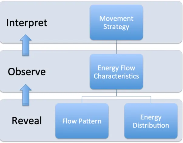
The main purpose of this research is to propose a new convention of the energy
flow model for intuitively interpreting the movement strategy according to the observed
energy flow characteristics. The energy flow characteristics refer to the flow pattern
and energy distribution among joints and segments. Research procedure is shown in
Figure 1-2. The proposed model utilizes a new perspective for bridging the joint and
segmental energetics in order to make each term of energy flow within the new model
easy to comprehend. Consequently, interpreting movement strategy will become very
intuitive. Another feature of the new model will be easy to implement. The
advantages of the new model will be demonstrated via analyzing the gait trials of
healthy young adults and elders walking at different speeds. The proposed energy
flow model will have a significant impact on improving the design of assistive devices
for locomotion and suggesting clinical interventions on rehabilitation, orthopedics, and
sports medicine.
In order to demonstrate how to utilize the proposed model to interpret the
movement strategy, the first clinical application is to investigate the utilization of ankle
power generated during push-off by using a new symbolic convention of energy flow
diagram. We used energy flow analysis techniques developed by Winter and
Robertson [1]. In addition to improving the clarity of visual presentation of the energy
flow analysis, we proposed a new symbolic convention to provide a self-interpreting
energy flow diagram. This diagram, with the new convention, would manifest the flow
of mechanical energy and how joint power is utilized in the leg by combining the joint
and segmental energetics. It was hypothesized for the experiment that the ankle power
generated during push-off would primarily increase the energy of ipsilateral limb
segments rather than the pelvis. To test this hypothesis, an energy flow diagram was
constructed from the data collected at the instant of peak ankle power generation, and
the ankle power utilization was then analyzed.
The second clinical application is to identify the important factors that control the
swing leg and to compare the energy flow characteristics of the swing phase during
level walking in young adults and the elderly. Factor analysis would be utilized to
extract the characteristics of the energy flows from a high-dimensional dataset. Our
doi:10.6342/NTU201901683
10
research hypothesis was that the elderly presents distinct energy flow characteristics
that unveil the altered coordination among the segments of the lower extremity during
the swing phase. Our work would help to facilitate the understanding of the
neuromuscular adaptation due to aging, which can potentially contribute to the fall
prevention, orthopedic treatments and rehabilitation interventions for elderly.
Figure 1-2 Research procedure of this project. The movement strategy will be interpreted by observing energy flow characteristics in terms of flow pattern and
energy distribution
Chapter 2
Materials and Methods
2.1 Subjects
Healthy young adults and healthy elders were recruited in this research. Exclusion
criteria included the inability to follow instructions, cardiopulmonary dysfunctions,
joint replacements in the lower extremities, arthritis, diabetes, vestibular deficits, or any
type of neuromusculoskeletal problems that could interfere with the gait pattern. All
the participants were right foot dominant, defined as the preferred leg for kicking a ball.
The experimental protocol was approved by and performed in accordance with the
relevant guidelines and regulations of the Research Ethics Committee of National
Taiwan University Hospital (No. 201112121RIC). All subjects had provided their
signed informed consents before participating in the study. The blank informed
consent was shown in Appendix I.
2.2 Instrumentation
Two optoelectric position sensors (Optotrak Certus, Northern Digital Inc.,
Waterloo, Canada) were used to collect kinematic data during gait (Figure 2-1.a).
doi:10.6342/NTU201901683
12
Rigid bodies which contain three infrared-emitting diodes (IRED) in each set are
respectively attached on lower limb segments (Figure 2-1.b) and thus the segment-fixed
coordinate systems can then be established and tracked. By finishing the procedure
of digitizing segmental landmarks while the presence of the rigid bodies at static
standing posture (Figure 2-1.d), spatial coordinates of segmental landmarks can then
be tracked. Kinetic data were collected with two force platforms (Accugait, Advanced
Mechanical Technology Inc., Massachusetts, USA) (Figure 2-1.c). Both kinematic
and kinetic data were collected synchronously at the sampling rate of 50 Hz via a
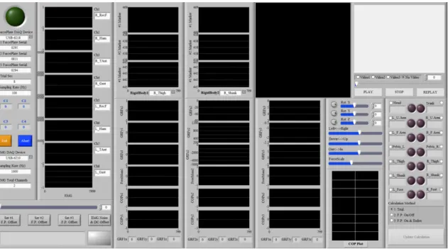
program developed in LabVIEW 14.0 (National Instruments, Texas, USA) (Figure 2-
2). An overview of the instrumentation setup in this research was shown in Figure 2-
3.
Figure 2-1 (a) Optoelectric position sensor to track marker trajectory ; (b) rigid bodies
that contain three active markers in each set ; (c) force plates that are embedded in the
floor ; and (d) Apply rigid bodies on the subject.
Figure 2-2 LabVIEW program developed to collect gait trials for energy flow analysis
doi:10.6342/NTU201901683
14
Figure 2-3 An overview of the instrumentation setup in this research
2.3 Experimental Protocol
All subjects walked with shoes along a 10-meter walkway at the self-selected
speed and the fast speed respectively. The instruction for the fast speed was to ask the
subject simulating a functional task, i.e. crossing a street as fast as possible when the
green light is about to turn red in 10 seconds. Each subject was allowed to practice
and completed at least three successful gait trails. A trial was considered "successful"
when constant walking speed was obtained during gait.
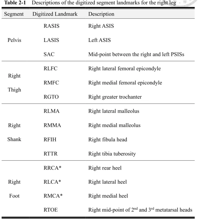
Table 2-1 showed the 14 segmental landmarks that were digitized for capturing
body motions. Trajectories of all the landmarks were recorded and filtered with a
fourth-order, bidirectional Butterworth low-pass filter with a cutoff frequency of 10 Hz.
Origins and definitions of each segmental coordinate system determined by the
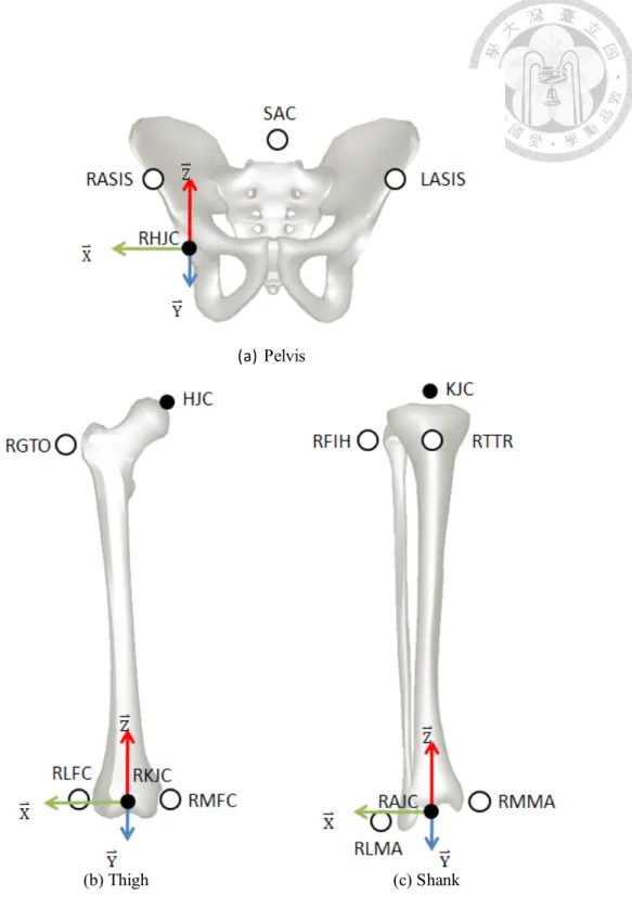
digitized segmental landmarks are listed in Table 2-2. The illustrations of each
segmental coordinate system together with the placements of the digitized landmarks
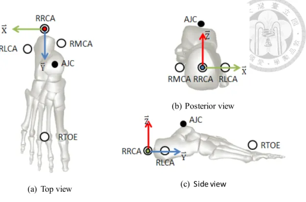
are also shown in Figure 2-4 and Figure 2-5.
The kinematic data were obtained by calculating the orientations of segmental
coordinate system. The mass and inertial properties were individually calculated with
reference to the coefficients from previous literature [39]. The kinetic data including
doi:10.6342/NTU201901683
16
joint force, moment, and power are analyzed by the methodology of inverse dynamics.
Table 2-1 Descriptions of the digitized segment landmarks for the right leg Segment Digitized Landmark Description
Pelvis
RASIS Right ASIS
LASIS Left ASIS
SAC Mid-point between the right and left PSISs
Right Thigh
RLFC Right lateral femoral epicondyle RMFC Right medial femoral epicondyle RGTO Right greater trochanter
Right Shank
RLMA Right lateral malleolus RMMA Right medial malleolus RFIH Right fibula head RTTR Right tibia tuberosity
Right Foot
RRCA* Right rear heel RLCA* Right lateral heel RMCA* Right medial heel
RTOE Right mid-point of 2nd and 3rd metatarsal heads
* Vertical coordinates of RRCA, RLCA, and RMCA at neutral position are equal
Table 2-2 Origins and definitions of segmental coordinate system for the right leg
Segment Origin Definition
Pelvis
Right hip joint center (RHJC) determined by the method proposed by Bell et al. [40]
The unit vector of the line passing from LASIS to RASIS The unit vector of the cross
product of the and The unit vector superiorly normal
to the plane containing RASIS, LASIS, and SAC
Right Thigh
Right knee joint center (RKJC) determined by the mid-point of RLFC and RMFC
The unit vector of the line passing from RMFC to RLFC The unit vector anteriorly normal
to the plane containing RGTO, RLFC, and RMFC
The unit vector of the cross product of the and
Right Shank
Right Ankle Joint Center (RAJC) determined by the mid-point of RLMA and RMMA
The unit vector of the cross product of the and the line passing from RAJC to RTTR The unit vector anteriorly normal
to the plane containing RFIH, RLMA, and RMMA
The unit vector of the cross product of the and
Right
Foot RRCA
The unit vector of the cross product of the line passing from RRCA to RTOE and
The unit vector of the cross product of the and
The unit vector superiorly normal to the plane containing RRCA, RLCA, and RMCA
doi:10.6342/NTU201901683
18
Figure 2-4 Illustrations of segmental coordinate systems and the digitized landmarks for the (a) pelvis, (b) right thigh, and (c) right shank in A-P view
(a) Pelvis
(b) Thigh (c) Shank
Fig. 3.1 Illustrations of segmental ACSs and the digitized landmarks for (a)the pelvis, (b)right thigh, and (c)right shank in A-P view
Figure 2-5 Illustrations of segmental coordinate system and the digitized landmarks for the right foot in (a) top view, (b) posterior view, and (c) side view
(a) Top view
(b) Posterior view
(c) Side view
Fig. 3.2 Illustrations of segmental ACS and the digitized landmarks for right foot in (a)top view, (b)posterior view, and (c)side view
doi:10.6342/NTU201901683
20
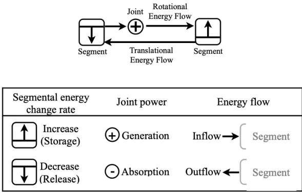
2.4 Energy Flow Model
The energy flow diagram likens potential and kinetic energy to a fluid, while body
segments are likened to tanks that can store and release this fluid. The joints are
likened to flow sources and sinks, and the mechanical work that transmits energy
between body segments through joint forces and moments are like monoarticular pipes
that the fluid flows through between the tanks, hence the term energy flow. The
diagram can reveal the energy distribution over multiple segments, simultaneously.
2.4.1 Detailed energy flow diagram
A new symbolic convention of the detailed energy flow diagram which has four
core elements, namely translational energy flow (TF) mediated by joint forces,
rotational energy flow (RF) mediated by joint moments, segmental energy change
rate, and joint power was proposed in this research. TF was calculated by TF = 𝐹 ∙
𝑣( , whereas 𝑣( is the linear velocity of a joint center and F is the joint force. TF is
the power used to transmit the joint force while producing the translational movement
in the direction of energy flowing across a joint. In a detailed energy flow diagram
(Figure 2-6), the horizontal arrows that directly connect the body segments represent
translational energy flow.
RF was calculated by 𝑅𝐹 = 𝑀 ∙ 𝜔,, whereas ωs is the angular velocity of a
segment and M is the joint moment. In a detailed energy flow diagram (Figure 2-6),
the horizontal arrows connecting the segments through the joints represent the
rotational energy flow. For either translational or rotational energy flow, a positive
(negative) value represents an inflow (outflow) of energy to a segment. For either
translational energy flow or rotational energy flow, the direction of a horizontal arrow
is determined by the sign of the value obtained from energy flow analysis. For instance,
the arrow direction of a positive energy flow shall be toward a segment, which also
means the energy is flowing into the segment.
Figure 2-6 A new symbolic convention of the detailed energy flow diagram.
doi:10.6342/NTU201901683
22
The segmental energy change rate ( ) is for the change of the total mechanical
energy of a segment. Total mechanical energy refers to the sum of potential energy (PE),
translational kinetic energy (TKE), and rotational kinetic energy (RKE). PE was
calculated by 𝑃𝐸 = 𝑚𝑔ℎ, whereas m is the mass of a segment, g is the gravitational
acceleration, and h is the height of the center of mass of a segment. TKE was calculated
by 𝐸 =23𝑚𝑣,∙ 𝑣, , whereas 𝑣, is the linear velocity of a segment’s center of mass.
RKE was calculated by 𝐾𝐸 =23𝜔,∙ 𝐼𝜔, , whereas I is the moment of inertia of a
segment. In a detailed energy flow diagram (Figure 2-6), squares represent different
body segments where the direction of a vertical arrow within a square is determined by
the sign of the value of the corresponding segmental energy change rate. For example,
the arrow direction of positive segmental energy change rate is upward, which also
means that the segmental energy is increasing, i.e. energy storage.
Joint power (JP) was calculated by 𝐽𝑃 = 𝑀 ∙ 𝜔( whereas ωj is the angular
velocity of a joint. The role of joint power is to modulate rotational energy flow across
a joint. A positive (negative) joint power refers to power generation (absorption) by
muscles. In our energy flow model, the joint power also equals to the sum of proximal
RF of the distal segment and distal RF of the proximal segment, e.g., JPknee = RFshank,
E!s
proximal + RFthigh, distal. This equation can help to clarify the role of joint power on rotational energy flow. In a detailed energy flow diagram (Figure 2-6), circles
represent joints, and ‘+’ and ‘-’ symbols indicate whether the joints generate (symbol:
+) or absorb (symbol: -) energy.
By connecting ankle joint power with other energetic elements, the utilization of
ankle power can be intuitively tracked within the proposed detailed energy flow
diagram like a map, which further describes movement strategy of walking during ankle
push-off.
doi:10.6342/NTU201901683
24
2.4.2 Simplified energy flow diagram
In order to ease the observation of the energy flow characteristics, the detailed
energy flow diagram can be further simplified by merging translation energy flow and
rotational energy flow into either segmental proximal flow ( ) or segmental distal
flow ( ). The segmental proximal/distal flow was calculated by:
𝐸̇8(𝑜𝑟 𝐸̇=) = 𝐹 ∙ 𝑣( +𝑀 ∙ 𝜔,
The segmental proximal/distal flow indicates the energy entering or leaving a segment
at its proximal or distal part, which is easier to comprehend. Taking the thigh for
example, the positive thigh proximal flow ( ) represents there is an energy inflow
to the thigh at the hip joint, whereas the negative thigh distal flow ( ) represents
there is an energy outflow from the thigh to the knee joint (Figure 2-7).
Figure 2-7 Segmental proximal and distal flows in a simplified energy flow diagram
Ep
Ed
thigh
E!p,
thigh
E!d,
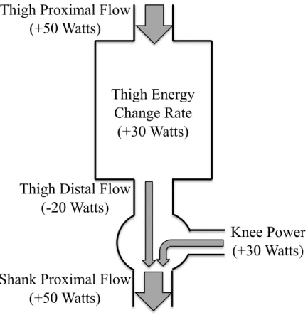
In a simplified energy flow diagram, the segmental energy change rate ( ) equals
to the summation of segmental proximal and distal flows of a segment, i.e.
. For example, 50 Watts of and -20 Watts of indicate that
increases 30 Watts (Figure 2-8). It allows us to look into the regulation of the
segmental energy. Through this observation, we can study how the energy flow
modulates the potential energy and kinetic energy of the segment.
Figure 2-8 An example of a simplified energy flow diagram including the thigh and the knee joint.
E!s
p d
s E E
E! = ! + ! E!p, thigh E!d, thigh
thigh
E!s,
Thigh Proximal Flow (+50 Watts)
Thigh Distal Flow (-20 Watts)
Thigh Energy Change Rate
(+30 Watts)
Shank Proximal Flow (+50 Watts)
Knee Power
(+30 Watts)
doi:10.6342/NTU201901683
26
In a simplified energy flow diagram, a positive joint power can result in two kinds
of flow pattern across the joint in terms of a pure energy source and increasing
transferring energy. In contrast, a negative joint power can result in two kinds of flow
pattern across in terms of a pure energy sink and decreasing transferring energy. The
amount of power leaving the joint equals that entering the joint, i.e., the joint power
equals to the summation of of the distal segment and of the proximal segment,
e.g. . For example, 50 Watts of and -20 Watts of
represent that the knee generates 30 Watts of power ( )(Figure 2-8).
Figure 2-9 showed another example of the energy flow characteristics presented
by the energy distribution and flow pattern in a simplified energy flow diagram. It is
effortless to conclude that the energy stored in the thigh and the shank is contributed by
the power generation of knee muscle. The example demonstrates that the proposed
energy flow model provides an intuitive way to observe joint power utilization.
Otherwise, either the role of joint power or the source of segmental energy change may
remain ambiguous if not bridging joint and segmental energetics together.
Another format of presenting the energy flow pattern of one leg was also adopted
in this research in order to intuitively link to the movement (Figure 2-10). Since there
Ep Ed
thigh d, shank p,
knee E E
P = ! + ! E!p,shank
Ed, thigh Pknee
is no foot distal flow during the swing phase, i.e. foot does not contact the ground, foot
energy change rate is identical to the foot proximal flow. Accordingly, there are
eleven energy flow elements in the swing leg model, including the pelvis distal flow,
hip power, thigh proximal flow, thigh energy change rate, thigh distal flow, knee power,
shank proximal flow, shank energy change rate, shank distal flow, ankle power, and
foot proximal flow.
Figure 2-9 A simplified energy flow diagram to reveal the energy source of the thigh and the shank
doi:10.6342/NTU201901683
28
Figure 2-10 A complete simplified energy flow diagram of one leg. All energy flows are presented in the positive direction.
!
Thigh Proximal Flow Pelvis Distal Flow
Thigh Distal Flow
Shank Distal Flow
Foot Distal Flow
Shank Proximal Flow
Foot Proximal Flow
Hip Power
Knee Power
Ankle Power Thigh
Energy Change
Rate (+)
Shank Energy Change Rate (+)
Foot Energy Change Rate (+)
2.5 Data Analysis
2.5.1 Construction of a detailed energy flow diagram at the instant of push-off
The translational energy flow, rotational energy flow, joint power, and segmental
energy change rate were analyzed. Energy flow between the foot and ground were
calculated based on techniques in the literatures that account for energy dissipated in
foot deformation [41-43]. The detailed energy flow diagram was constructed at the
instant of peak ankle power generation since such instant is considered representative
of push-off phase [44-46]. Subsequently, the distribution of ankle power generated
during push-off was further investigated by analyzing the mechanical energy of each
segment. These analyses were performed to reveal how ankle power was utilized and
to test whether the ankle power generated during push-off delivered substantial
propulsive energy to the pelvis.
2.5.2 Factor analysis of the energy flow characteristics in swing phase
The kinematic data that was used to calculate the energy flow were normalized to
the duration of the swing phase (yielding the relative time profiles between 0% and
100%) and were averaged over the three recorded trials. The energy flow data of all
doi:10.6342/NTU201901683
30
subjects were then normalized to the subject’s body mass, and averaged according to
the normalized time profiles at 1 percent interval along with the swing duration. A
correlation coefficient matrix derived from the normalized averaged data of all the 11
energy flow elements in the swing leg model would be produced to evaluate the
correlation between each of the energy flow element. The correlation coefficient
ranges from 0 to 1 and the higher coefficient indicates the greater correlation. The
correlation matrix would be used as inputs for the factor analysis. By rotating the
principal components, factor analysis is then utilized to extract the characteristics of a
high-dimensional dataset. The extracted 1st and 2nd factors indicate the first two most
prominent energy flow patterns of the entire swing phase. For each factor, energy
flow elements with significant absolute loadings (> 0.8) would further be depicted in
the energy flow model while the sign of the loading determined the flow direction of
the corresponding energy flow element. Consequently, the energy flow characteristics
of the swing leg can be intuitively observed corresponding to each of the extracted
factors. The independent t-test was used to compare the walking speeds between the
young adults and the elderly.
2.5.3 Verification of the proposed energy flow analysis
This research has developed a software program to perform the proposed energy
flow analysis (Figure 2-11). Nevertheless, it would be difficult to judge the robustness
of the data if the accuracy of our energy flow analysis technique was not verified. Our
energy analysis technique was verified by comparing the segmental energy change rates
calculated from kinematic data with the summation of the corresponding energy
inflow/outflow that are calculated via inverse dynamics. Since the segmental energy
change rate was analyzed via simple calculations, it was less prone to error. Thus, the
accuracy of developed technique can be assured if the results from both calculations
are similar. In previous literatures, the discrepancy between these two calculating
methods was called power imbalance. Theoretically, the power imbalance is zero
since either calculation follows the principles of rigid-body dynamics.
Figure 2-12 showed the segmental energy change rates of thigh, shank, and foot
from a gait trial of a young healthy adult, in which data is processed by our developed
software. The results showed that each segmental energy change rate was highly
matched with the summation of the corresponding energy inflow/outflow. Since
nearly zero power imbalance was achieved, the accuracy of developed technique was
doi:10.6342/NTU201901683
32
assured. Another comparison of segmental energy change rates cited from the other
research [47] was showed in Figure 2-12 for reference.
Figure 2-11 The user interface of the developed energy flow analysis software.
Chart and value of each energy flow within the proposed model can be conveniently
assessed via the software. In addition, 3D animation of gait is shown together with
ground-reaction-forces in order to distinguish which gait event is being analyzed.
(a)
(b)
(c)
Figure 2-12 Segmental energy change rate of (a) thigh, (b) shank, and (c) foot
calculated by inverse dynamics (dash-line) and kinematic data (dot-line). Charts from
both calculations were highly matched, i.e. nearly zero power imbalance.
-0.6 -0.4 -0.2 0.0 0.2 0.4 0.6 0.8
1 100
Energy (W/kg)
Gait Cycle (%) Energy change rate of the thigh
Inverse Dynamic Kinematic
-1.0 -0.5 0.0 0.5 1.0 1.5
1 100
Energy (W/kg)
Gait Cycle (%)
Energy change rate of the shank
Inverse Dynamic Kinematic
-1.2 -1.0 -0.8 -0.6 -0.4 -0.2 0.0 0.2 0.4 0.6 0.8
1 100
Energy (W/kg)
Gait Cycle (%) Energy change rate of the foot
Inverse Dynamic Kinematic
doi:10.6342/NTU201901683
34
Figure 2-13 Comparison of segmental energy change rates cited from the other research [47]. Considerable power imbalance existed in the stance phase for all
segments whereas nearly zero power imbalance in the swing phase.
Chapter 3
Mechanical energy utilization of ankle push-off in young adults
3.1 Detailed energy flow diagram during ankle push-off
The gait data for this clinical application of energy flow analysis were collected at
self-selected speeds (1.43±0.09 m/s) from 8 healthy young adults (Age: 23±2 years old,
Gender: male). The energetic data obtained from the developed energy flow model
(Appendix II) were used to construct the detailed energy flow diagram at the moment
of peak ankle power generation (Figure 3-1).
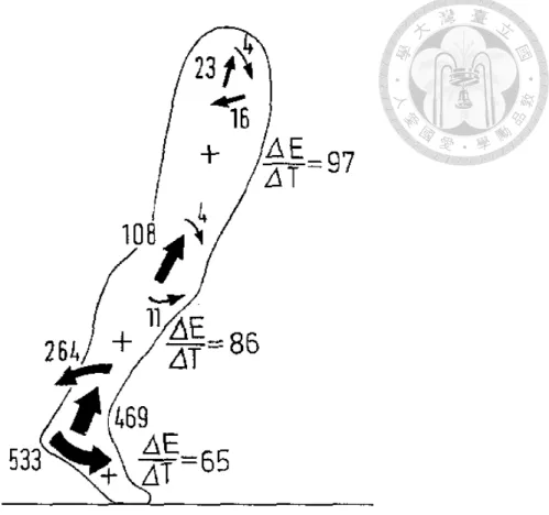
Figure 3-1 A detailed energy flow diagram at the peak of ankle power generation during push-off. All values are reported in power normalized by body weight (W/kg) either above or below their corresponding symbol. Reported values are the average across subjects.
Thigh Shank Foot
+
Ankle
0.13 1.00 1.29
Ground 0.42
Knee
+ -
Hip
Pelvis
2.78 1.52
1.21 Opposite
Leg 0.04
Trunk
Thigh Shank Foot
+
Ankle
0.13 1.00 1.29
Ground 0.42 6.72
Knee
0.27
+ -
Hip
0.36 Pelvis
2.78 1.52
1.21 Opposite
Leg 0.05
6.89 0.01
4.11 1.29
0.08
Trunk
1.05 0.47
0.17 2.61 1.32
0.93
0.28 0.07
a
b
Segmental energy
change rate Joint power Energy flow
+
-
Absorption Generation Increase(Storage) Decrease
(Release) Outflow
Inflow
Segment Segment
Thigh Shank Foot
+
Ankle
0.13 1.00 1.29
Ground 0.42
Knee
+ -
Hip
Pelvis
2.78 1.52
1.21 Opposite
Leg 0.04
Trunk
Thigh Shank Foot
+
Ankle
0.13 1.00 1.29
Ground 0.42 6.72
Knee
0.27
+ -
Hip
0.36 Pelvis
2.78 1.52
1.21 Opposite
Leg 0.05
6.89 0.01
4.11 1.29
0.08
Trunk
1.05 0.47
0.17 2.61 1.32
0.93
0.28 0.07
a
b
Segmental energy
change rate Joint power Energy flow
+
- Absorption Generation Increase
(Storage) Decrease
(Release) Outflow
Inflow
Segment Segment
Thigh Shank Foot
+
Ankle
0.13 1.00 1.29
Ground 0.42
Knee
+ -
Hip
Pelvis
2.78 1.52
1.21 Opposite
Leg 0.04
Trunk
Thigh Shank Foot
+
Ankle
0.13 1.00 1.29
Ground 0.42 6.72
Knee
0.27
+ -
Hip
0.36 Pelvis
2.78 1.52
1.21 Opposite
Leg 0.05
6.89 0.01
4.11 1.29
0.08
Trunk
1.05 0.47
0.17 2.61 1.32
0.93
0.28 0.07
a
b
Segmental energy
change rate Joint power Energy flow
+
-
Absorption Generation Increase(Storage) Decrease
(Release) Outflow
Inflow
Segment Segment
doi:10.6342/NTU201901683
36
3.2 Energy flow between the shank and the foot
There was an energy flow loop between the shank and the foot where energy
moved from the shank to the foot through rotational energy flow as well as where
energy moved back to the shank from the foot through translational energy flow (Figure
3-1). Within the loop, the ankle power (2.78±0.22 W/kg) joined the rotational energy
outflow from the shank (4.11±0.80 W/kg) and produced an augmented energy inflow
to the foot of 6.89±1.06 W/kg. A small portion of this augmented energy flow
powered the motion of the foot (0.13±0.04 W/kg), and even less of that was transmitted
to the ground (0.05±0.22 W/kg). However, the majority of this augmented energy was
transmitted to the shank through translational energy flow (6.72±0.96 W/kg). In other
words, this translational energy flow was transformed from the rotational energy flow
induced by ankle muscles as shown in the energy flow loop. The energy flow loop
between the shank and the foot is the energetic representation of ankle plantarflexor
moment (producing rotational power) inducing the upward ankle reaction force
(producing translational power) on the shank through the lever action of the foot.
3.3 Utilization of ankle power
The detailed energy flow diagram (Figure 3-1) shows how energy moved from the
lower leg segments all the way up to the pelvis through translational energy flow, which
could be considered the “push-off” power. However, we found that the magnitude of
translational energy flow moving from the shank to the thigh (0.27±0.51 W/kg) was
only about 10% of the ankle power (2.78±0.22 W/kg). The majority of ankle power
either increased the mechanical energy of the shank (1.29±0.24 W/kg, about 46%) or
was absorbed by the knee (1.05±0.51 W/kg, about 38%). The remaining ankle-
induced power moved from the shank to the thigh through translational energy flow
(0.27±0.51 W/kg) and was combined with power generated from the hip (1.29±0.34
W/kg) to increase the mechanical energy of the thigh (1.00±0.19 W/kg). Although
the translational energy flow from the thigh to the pelvis (0.36±0.61 W/kg) transmitted
some of the ankle joint power to the pelvis, the detailed energy flow diagram (Figure
3-1) clearly illustrates how the majority of power generated by the ankle during push-
off flowed to the ipsilateral leg and how little of that was transmitted toward the trunk.
doi:10.6342/NTU201901683
38
3.4 Energy flow of the pelvis
The utility of the energy flow diagram is that it graphically reveals the flow of
energy through the entire leg, rather than focusing on a single joint or segment.
However, one energy flow diagram only represents one instant at a time. In order to
verify that our results are not unique to this single instant, we examined the translational
energy flow from the trailing thigh to the pelvis during the entirety of push-off (Figure
3-2). We found that the translational energy flow applied to the pelvis was small
compared to ankle power, and that energy only flowed into the pelvis for less than a
half of the duration of push-off. We also examined the rotational energy flow between
the pelvis and trailing thigh, and found that a small amount of energy was consistently
flowing from the pelvis to the hip during the entirety of push-off (Figure 3-2).
Figure 3-2 Ankle power and the energy transmitted to the pelvis. The light gray
area indicates the period of push-off and the dark gray area indicates the duration of the
translational energy inflow (positive value) to the pelvis. Standard deviations are
shown as vertical bars. It can be observed that how much power generated by the
ankle during push-off and how little power transmitted to the pelvis.
doi:10.6342/NTU201901683
40
3.5 Segmental energetics
To better understand the utilization of ankle power generated during push-off, we
assessed the energy compositions of each segment in terms of potential energy and
kinetic energy (Figure 3-3a-3d). The change in the total mechanical energy of the
pelvis (-0.0222 J/kg) before and after push-off (Figure 3-3a) were dominated by the
change in kinetic energy (-0.0225 J/kg). Furthermore, we found that such change in
kinetic energy was largely determined by the change of the translational kinetic energy
(-0.0225 J/kg), especially in the anterior-posterior direction (-0.0223 J/kg), while the
change in rotational kinetic energy was several orders of magnitude smaller (<0.0001
J/kg) (Figure 3-3e).
doi:10.6342/NTU201901683
42
Figure 3-3 Energy characteristics of human gait. (a)-(d) The mechanical energy
compositions of the pelvis, thigh, shank, and foot, respectively. (e) The composition of
translational kinetic energy of the pelvis in terms of the anterior-posterior (A-P),
medial-lateral (M-L), and vertical directions. The light gray area indicates the period
of push-off. Standard deviations are shown as vertical bars.
3.6 Discussion
At the instant of ankle peak power generation, our energy flow diagram showed
that the ankle power was an important source of power for the motion of the ipsilateral
leg. The ankle power supplied most of the energy required by the foot (0.13±0.04
W/kg) in the form of the rotational energy flow since another energy inflow from the
ground was relatively small (0.01±0.03 W/kg) (Figure 3-1). We also found that the
ankle power transformed into translational energy flow (6.72±0.96 W/kg) at the ankle
joint, and such translational energy flow was the sole energy inflow to supply the energy
required for the motion of the shank (Figure 3-1). As for the thigh, the hip-induced
rotational energy flow (1.29±0.24 W/kg) and the translational energy flow (0.27±0.51
W/kg) from the shank were both energy sources (Figure 3-1). Our study gives a
clinical application on how to use the energy flow diagram with the proposed
convention to link joint energetics to segment energetics so that the movement strategy
can be further explained. Since most of the ankle power supplies energy to ipsilateral
foot, shank, and thigh, it can be readily inferred that the ankle power generated during
push-off mainly propels the trailing leg forward as it transitions from stance to swing
phase.
doi:10.6342/NTU201901683
44
The purpose of examining pelvic energetics was to assess the role played by ankle
power on forward propulsion. Based on the kinematics, we calculated that the
mechanical energy of the pelvis decreased (0.42±0.24 W/kg) at the moment of peak
ankle power (Figure 3-1), and such decrease was largely determined by a decrease in
kinetic energy (Figure 3-3e), indicating that the upper body is decelerating during push-
off. Furthermore, we found that the trailing leg only performed positive work on the
pelvis for less than half of the push-off period (Figure 3-2) and the net work performed
by the trailing leg on the pelvis during the push off period was negative. The positive
power supplied by the trailing leg was not enough to prevent the mechanical energy of
the pelvis from decreasing during push-off (Figure 3-3a). The positive work
performed by the trailing leg may mitigate some of the energy lost during double-limb
support, but such does not contribute to a net increase in kinetic energy which is often
associated with forward propulsion. Based on the distribution of power throughout
the trailing leg and the relatively small amount of energy transferred to the pelvis, it
implies that the primary role of ankle during push-off is to propel the trailing leg
forward rather than deliver substantial propulsive energy to the pelvis.
Our study analyzed the utilization of ankle power generated during push-off by
illustrating energy flow diagram in a new symbolic convention that combines core
mechanical energetic elements together. Another schematic energy flow diagram was
used previously [1]; however, the choice of symbols and the close proximity of the
different symbols as well as numbers made identifying the different quantities and the
direction of rotational energy flow difficult. The regular structure of our diagram
eliminates such confusion; our symbolic convention clearly and readily shows where
energy is increasing, where it is transferred to, and where it is generated or absorbed.
Our symbolic convention in the diagram facilitates the conceptualization of mechanical
energy transfer between body segments as water flowing through a system of pipes,
storage tanks, and pumps. Such comparison allows readers use their understanding of
a more familiar system and fluid flow to intuit energy transfer within the body. In
addition, it eases the interpretation of energy flow analysis, especially when comparing
energy flow characteristics of different movements or subject groups. Comparing
energy flow patterns of various gait events between the able-bodied and patients with
neuromuscular disorders would require numerous energy flow diagrams lining up
together in order to discern the movement strategy. We expect that the symbolic
convention in the energy flow diagram can give a more succinct and standardized
doi:10.6342/NTU201901683
46
representation than the previous diagram.
Another benefit of the symbolic convention in the energy flow diagram compared
to alternative energy analysis techniques [18, 48] is the ability to show where and how
energy has been transmitted during a movement, especially for the energy flow across
adjacent segments. Thus, current techniques allow us to better explore the role of
ankle during push-off in relation to other segments to be analyzed. For example, the
ankle power generated during push-off can be tracked to demonstrate the power
utilization shown in the energy flow diagram, which provides evidences to support
previous studies that suggested the role of the ankle during push-off primarily
contributes to the initiation of swing [16–19]. A previous study also yielded similar
results in the push-off period which claimed that the power was generated at the hip
and the ankle, absorbed at the knee, and very little was transferred to the trunk [1].
However, the joint power magnitudes of the knee and the hip from the previous study
[1] were much smaller than those of this study partly since the previous study performed
the analysis at some point in late push off, while our analysis was carried out at peak
ankle power generation. Differences in equipment may also account for the
discrepancy, as the contemporary digital 3D motion capture used in this study is more
precise than the hand digitizing of markers from cine film, which was used in the
previous study [1]. Differences are also attributed to the fact that our research took
the energy dissipated in foot deformation into account. Our reported values of joint
power compare better with those from a more recent investigation [5] than those from
the previous study [1].
Several limitations of this research should be addressed in the future.
Calculations of joint center velocity differ slightly between proximal and distal
segments, which results in a discrepancy in the translational energy flow between those
segments. The only discrepancy with significant figures was a 0.27 W/kg difference
in the translational energy flow between the proximal shank and the distal thigh.
Nevertheless, this discrepancy does not affect our findings since the direction of the
translational energy flow from the shank to the thigh is consistent between the proximal
shank and distal thigh. Therefore, in order to simplify the diagram, we only show the
translational energy flow values calculated from the proximal end of the segments.
Regardless of the source of such energy flow discrepancy is from the physical
translation within the joint or the limitations of rigid body assumptions [49], a more
recent study has found that taking account of the energy flow discrepancy can better
doi:10.6342/NTU201901683
48
capture energy changes of the body [48].
Another limitation of this study is that only the energy flow of trailing leg was
presented. Nevertheless, ignoring the energy flow of the leading leg does not affect
our results on the pelvis energetics even if the leading leg transmits energy to the pelvis
during push-off due to the fact that we calculate the mechanical energy of the pelvis by
pelvis kinematics only. In addition, the validity of the energy flow analysis has to be
rigorously checked before applying to other areas such as sports or rehabilitation
medicine, given our analysis was performed on the basis of limited number of healthy
subjects. In order to give a more comprehensive example of applying our new
symbolic convention, a future work of the whole body energy flow diagram at different
gait phases is warranted.