GOODS天區次毫米波星系的聚集

(1)

國立臺灣大學理學院物理研究所碩士論文

Department of Physics College of Science

National Taiwan University Master Thesis

GOODS 天區次毫米波星系的聚集

Angular Clustering of Submillimeter Galaxies in GOODS Fields

鄭偉良 Wei-Leong Tee

指導教授：闕志鴻教授 (國立臺灣大學) Advisor: Tzi-Hong Chiueh, Professor (NTU)

共同指導教授：王為豪副研究員 (中央研究院天文及天文物理研究所)

Co-Advisor: Wei-Hao Wang, Associate Research Fellow (ASIAA)

中華民國 107 年 1 月 January, 2018

(2)

(3)

國立臺灣大學碩士學位論文口試委員會審定書

GOODS 天區次毫米波星系的聚集

Angular Clustering of Submillimeter Galaxies in GOODS Fields

本論文係鄭偉良君 (R04222026) 在國立臺灣大學物理研究所完成之碩士學位論文，於民國 107 年 1 月 4 日承下列考試委員審查通過及口試及格，特此證明

(4)

(5)

誌謝

首先要感謝偉大的老闆們，王為豪副研究員和闕志鴻教授沒有放棄我。王為豪副研究員是一位非常有耐心且善解人意的指導者，不會讓學生感到壓迫，不吝於分享研究經驗，同時還能對研究給予極具建設性的看法和意見；闕志鴻教授待學生寬厚，富有同理心並願意努力為學生爭取權益，使學生能專心致志於研究上。我也要感謝口試委員們，

林彥廷副研究員和林俐暉副研究員對這項研究所提供的幫助以及所面對的問題，使這項工作能夠更加完善。我也很感激早年平下博之研究員所給予的中研院暑期研究計畫的工作機會，讓我堅定了想要從事天文研究的想法。我也要感謝在碩士研究期間幫助過我的朋友、同伴、

學長姐，有林征發（Bobby）、羅文斌（Vincent）、林聖傑、侯冠州、邱

奕儂、胡耀傑（Jerry）以及天文數學館 R922 的室友們。與他們的學術討論促成了這篇工作的正確性，但我更珍惜與大家一起在荊棘滿佈的研究路上攜手前進的時光，當中的血淚交織、燒肝搞笑都是一生無法抹滅的回憶。

一路走來的研究路坎坷不斷、跌宕起伏，經歷多次的低潮後，終於抵達現在這一步。我非常感激我家人對我所做決定的支持，是因為有他們作為我的後盾我才能義無反顧地進行我想要的研究。我最後要感謝的是 Lia，陪伴我走過我對人生的迷惘時候，也不吝於與我分享她的生活，是她的仁慈和寬容救贖了我，讓我有勇氣向前踏穩自己的步伐，

去尋找我人生的下一個里程碑。

(6)

(7)

Acknowledgements

First and foremost, I would like to thank my advisors Dr. Wei-Hao Wang and Prof. Tzi-Hong Chiueh for their patience and support throughout years in graduate school. I also wish to acknowledge other members in my thesis committee, Dr. Yen-Ting Lin and Dr. Li-Hwai Lin, who provided extremely helpful information that contributed to the completion of this thesis. Valuable contributions to this work have also been brought by helpful discussions with Chen-Fatt Lim (Bobby), Wen-Ping Lo (Vincent), Sheng-Chieh Lin, Kuan- Chou Hou and I-Non Chiu during the course of writing this thesis, and it would not have been possible without their help and support. I also want to thank Dr. Hiroyuki Hirashita, who not only inspired me a lot but also gave me my first opportunity to do research as an undergraduate in the ASIAA Summer Student Program.

I would also like to thank my family for their love and support, in particular my parents who have never urged me to leave the academic field earlier, and always support me for any decision I made. I want to thank my friends and office-mates in R922 of Astronomy-Mathematics Building in NTU throughout the years, for providing mental support as well as welcome distractions during my time there, especially Yao-Chieh Hu (Jerry) companionship and care. Finally I would like to thank Lia, who have always accompanied and supported me, and helped me go through all those struggling moments.

(8)

(9)

摘要

次毫米波星系為一群於紅外波段非常明亮的星系。因為大氣層吸收帶影響，地面能觀測的窗口在遠紅外波段部分為次毫米波段

(10⁻⁶− 10⁻³ m)，主要受到水氣吸收影響。星系演化圖像中，恆星形

成過程會伴隨劇烈的紅外波段輻射，故次毫米波星系是瞭解星系演化極為重要的一環。我們使用來自 GOODS 天區 SCUBA-2 次毫米波星系

的觀測數據，結合使用 K_s紅外波段非活躍星系的數據，對兩者做相關

性研究，由此推導出星系的空間聚集半徑 r₀及星系可能存在的暗物質

暈 Mhalo大小。本研究發現次毫米波星系的聚集強度比文獻所提及的較

低。

(10)

(11)

Abstract

Submillimeter galaxies (SMGs) are high-redshift galaxies (z = 1− 4) with very bright flux densities in the submillimeter waveband. To study their nature and their role in the galaxies evolution history, we present an angular clustering measurement of SMGs in the GOODS-North and GOODS-South.

We make a 2.0 mJy and 0.5 mJy cut on 850 µm flux density and noise. The total available SMG sources are 141, with 75 in North and 66 in South. Due to the large uncertainties induced from small size target autocorrelation, we conduct a cross-correlation between target and tracer with larger size to effec- tively reduce the uncertainties. We use ∼ 2500 Ks-selected normal galaxies from deep infrared observations in each field. We derive the clustering lengths and linear galaxy biases of both populations, which lead to the estimation of the SMG clustering length of r₀ ∼ 4 − 5 h⁻¹Mpc. We find that SMGs do not cluster strongly as reported in previous studies, occupying dark matter halo mass of M_halo ∼ 10¹²M_⊙.

Key words: galaxies: evolution — galaxies: clusters — galaxies: high- redshift — submillimeter: galaxies

(12)

(13)

4.1 K_sGalaxy ACF . . . 29 4.2 SMG-K_sGalaxy CCF . . . 32 4.3 SMG ACF . . . 33 4.4 Blending Bias Effect on The Clustering Length and DM Halo Mass . . . 34 4.4.1 Power Law Method: ACF of SMG . . . 35 4.4.2 Large-scale Bias Method: Bias Evolution to Clustering Length . . 35 4.5 Clustering Result and Comparison to Previous Works . . . 37 4.6 Discrepancy and Improvement . . . 40

5 Conclusions 41

(15)

List of Figures

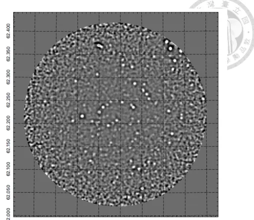
2.1 (a) GOODS-N 850 µm matched-filter S/N image. (b) GOODS-S 850 µm matched-filter S/N image. Both maps have radii about 10^′. . . 9 2.2 GOODS-N noise distribution, adopted from Cowie et al.(2017, their Fig.

1). (a) Azimuthally averaged 850 space after 850 µm rms noise vs. radius.

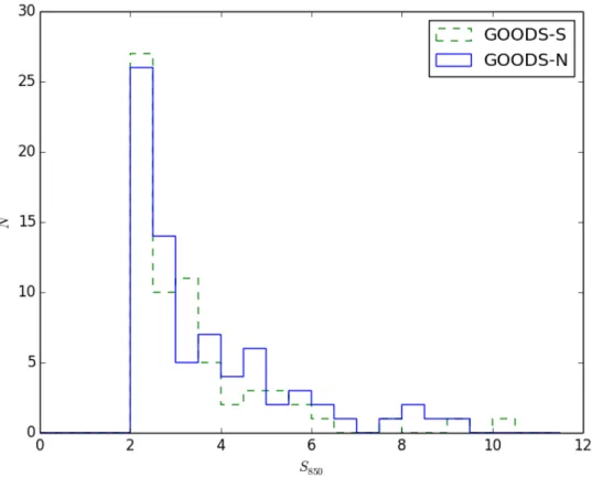
The more sensitive central region (radius less than 6^′) is dominated by the CV Daisy observations, while the outer region is covered by the PONG- 900 observations. The black dashed line shows the rms noise correspond- ing to a 4 σ detection threshold of 1.6 mJy, the approximate confusion limit for the JCMT at 850 µm. (b) Cumulative area covered vs. 850 µm rms noise. . . 10 2.3 SMG 850 µm flux density distribution. Blue solid line is the GOODS-

N SMGs flux distribution while green dotted line is for GOODS-S. The cut on 2 mJy is to avoid artificial clumping of sources due to observation pattern. Obviously our sample includes many faint SMGs S₈₅₀ < 4 mJy. . 10 2.4 (a) GOODS-N SMG sources map. (b) GOODS-S SMG sources map. The

inner green contour level is where σ_rms = 0.5 mJy. The red contour is the flux cut of S₈₅₀ = 2.0 mJy. Note that the surface density of sources is higher in the central low S/N region of the image. To account the apparent clumping toward the image center due to the observation method, we apply noise and S850 threshold cut on the image, remove the center- most faintest sources so that those relatively fainter S850 sources are also detectable at outer region. . . 11

(16)

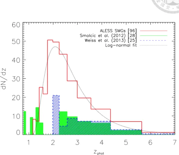
2.5 The redshift distribution of the ALESS SMGs, adopted from Simpson et al. (2014, their Fig. 12). The redshift distribution binned uniformly in time, and normalized by the width of each bin. Simpson et al. (2014) find the redshift distribution is well-represented by a log-normal distribu- tion with µ = 1.53± 0.02 and σz = 0.59± 0.01 . For comparison they show the redshift distribution from Smolčić et al. (2012), an interferometric study of 28 millimeter-selected SMGs, containing spectroscopic and photometric redshifts. They also show the spectroscopic redshift distribution from a similar interferometric study of 25 millimeter-selected lensed SMGs from Weiß et al. (2013), choosing the robust or best-guess redshifts from their analysis. They note that they have included the lensing probability as function of redshift, given in Weiß et al. (2013), in the distribution.

The SMG samples presented have selection functions that are difficult to quantify (especially the lensed sample of Weiß et al. (2013)), and hence do not have a well defined survey area. In contrast to the previous studies, the redshift distribution of the ALESS SMGs does not show evidence of a flat distribution between z ∼ 2–6, and displays a clear peak in the distribution at z = 2 . Brisbin et al. (2017) separately reported the similar phenomena for SMGs in COSMOS field, strengthen the reliability to use this redshift distribution in this study. . . 13

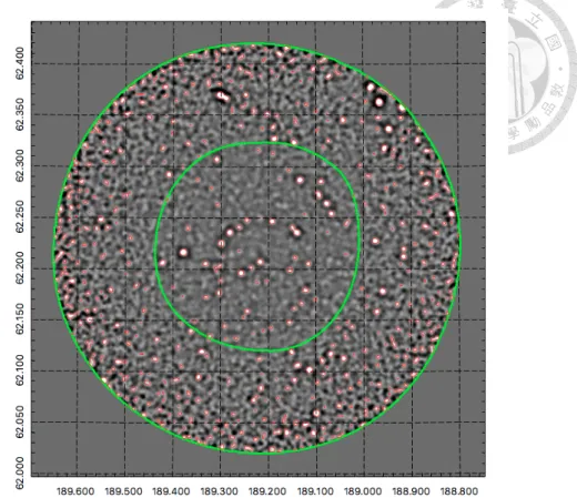
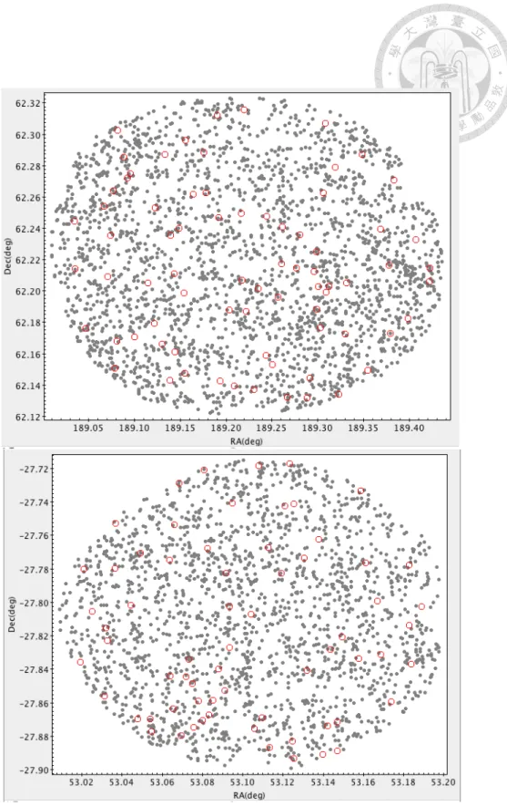
2.6 (a) GOODS-N (b) GOODS-S Two-dimensional distribution of SMGs and infrared normal K_sgalaxies in GOODS fields that are used in our analysis. The SMGs shown represent the subset of the full samples SMGs that have matched the noise and threshold cut. The K_sgalaxies are chosen to reside at z = 1−3 with 5 σ detection. The SMGs are shown here individ- ually with red circles while galaxies are in gray points. The blank areas represent the regions which are excluded from the analysis, i.e., around bright stars where few galaxies have been detected. . . 15

(17)

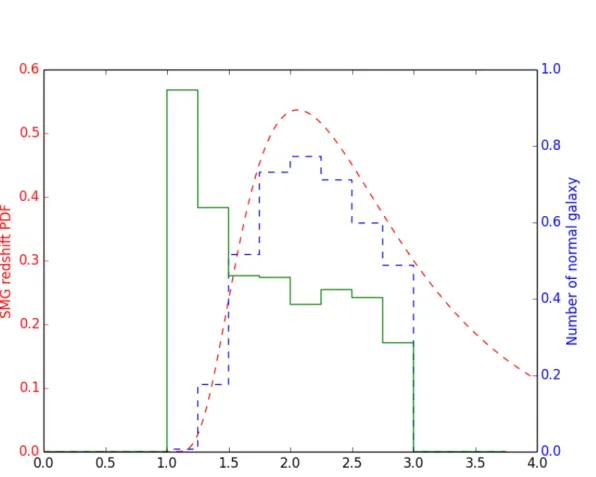
3.1 Redshift distributions for the K_sgalaxy sample in the redshift range z = 1− 3 (solid green line), and the SMG redshift distribution in the range z = 1− 4 (dotted red line). The histograms for all populations have been scaled so that the distribution can be directly compared to each others. Also shown is the redshift distribution for tracer galaxies (dashed blue line) selected to match the overlap in the redshift distributions of the SMGs, as used in both ACF and CCF analysis. 12% in GOODS-N and 20% in GOODS-S galaxies have spectroscopic redshifts. We use z_spec if any, otherwise z_photois used instead. . . 21

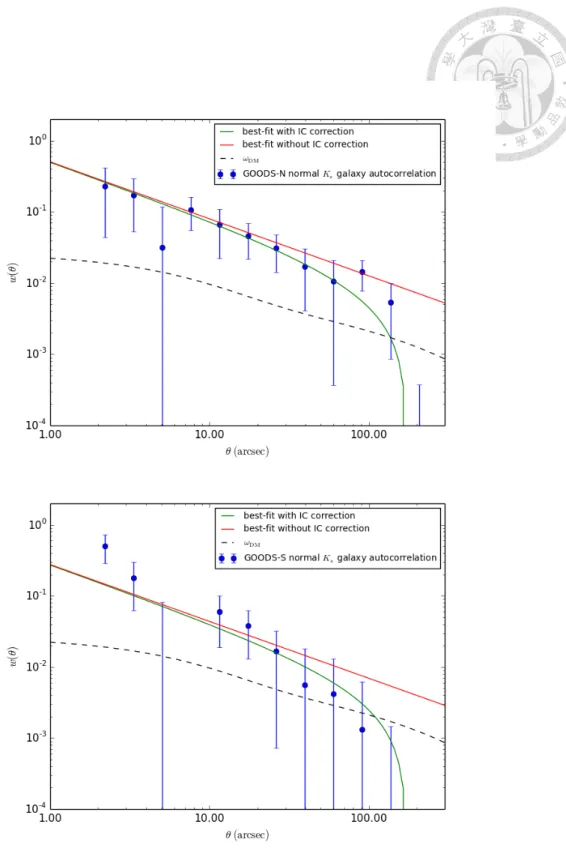
4.1 The ACF of K_s-selected normal galaxies in the GOODS fields. Galaxies are selected to match the overlap of the SMGs and galaxies in redshift space. Uncertainties are estimated from standard deviation of the bootstrap resampling result. The ACF of DM evaluated for the redshift distribution of the galaxies is shown by the dashed black line. The power law fit is performed on scales of 2^′′–100^′′ and is shown as the solid lines.

The green solid line is the best-fit power law model with the integral constraint (IC, consists of geometric factor ¯C) correction while red line is the one without correction. To reduce the downsizing amplitude effect arises from small survey area, we consider angle separation smaller than 100^′′. The observed amplitude of the K_sgalaxy ACF yields the absolute bias b_t, which we use to obtain the absolute bias bsand DM halo mass of the SMGs. 30

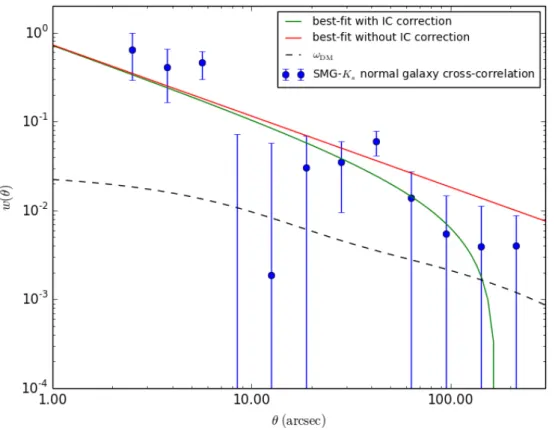
4.2 The CCF of SMG-K_sgalaxy. Uncertainties are estimated from standard deviation of the bootstrap resampling result. The ACF of DM, evaluated for the redshift distribution of the SMG, is shown by the dotted black line.

The power law fit was performed on scales 2^′′–100^′′ and is shown as the solid line. . . 32

(18)

4.3 The clustering length r₀ as a function of redshift. This figure shows the linear perturbation prediction of the evolution of clustering length and DM halos at large-scale. The z-positions of this work have been offset to exaggerate the difference. Red star is the clustering length of SMGs without blending correction, r0,SS; Blue diamond is the clustering length of SMGs with blending correction, r_0,SS,b ; Green circle is the clustering length of SMGs computed by large-scale bias with blending effect correc- tion,r_0,SS,L,b . Since we do not know the exact blending effect, we max- imize it according to Cowley et al. (2017) and estimate the smallest r₀ possible. The exact clustering length within 4− 6 h⁻¹Mpc. . . 36 4.4 Comparison of this work to the literature studies. The black points are

clustering results from previous studies: Webb et al. (2003); Blain et al.

(2004); Weiß et al. (2009); Williams et al. (2011); Hickox et al. (2012);

Wilkinson et al. (2017). The curves represent the predicted clustering strengths for DM halos of varying masses (labelled, in solar masses), produced using the formalism of Sheth et al. (2001). Colored regions are different galaxy populations illustrated in Hickox et al. (2012): LBGs at 1.5 < z < 3.5 (Adelberger et al. 2005), Multiband Imaging Photometer for Spitzer (MIPS) 24-µm-selected star-forming galaxies (SFGs) at 0 <

z < 1.4 (Gilli et al. 2007), typical red and blue galaxies at 0.25 < z < 1 from the AGN and Galaxy Evolution Survey (Hickox et al. 2009) and Deep Extragalactic Evolutionary Probe 2 (DEEP2; Coil et al. 2008) spec- troscopic surveys, luminous red galaxies (LRGs) at 0 < z < 0.7 (Wake et al. 2008) and low redshift elliptical galaxies with r-band luminosities in the range 1.5–3.5 L^∗, derived from the luminosity dependence of clustering presented by Zehavi et al. (2011). . . 39

(19)

List of Tables

2.1 Galaxy samples used in this study. We choose SMGs with S850 > 2mJy and σ < 0.5mJy. Infrared K_snormal galaxies (5σ) are chosen to reside in

the same area coverage, with 1 < z < 3. . . . 14

4.1 Result of K_s-selected near-infrared normal galaxies ACF. . . 31

4.2 Result of SMG-K_sgalaxy CCF and expected SMG ACF. . . 33

4.3 Results of clustering length, galaxy bias, and DM halo mass. . . 35

(20)

(21)

Chapter 1 Introduction

Submillimeter galaxies (SMGs) are a population of galaxies emit strongly in the far- infrared submillimeter wavebands and are ultraluminous infrared galaxies (ULIRGs; e.g., Smail et al. 1997; Barger et al. 1998; Hughes et al. 1998; Blain et al. 2002). They generally have high redshifts, with a redshift distribution appearing to peak at z ∼ 2.5 (e.g., Chap- man et al. 2003, 2005; Wardlow et al. 2011), so that SMGs are at their commonest around the same epoch as the peak in powerful active galactic nuclei (AGN) and quasi-stellar objects (QSOs). There are lots of recent works trying to investigate the evolutionary re- lationship across SMGs and other type of galaxies (e.g., Richards et al. 2006; Assef et al.

2011;Hickox et al. 2012). The immense far-infrared luminosities of SMGs are believed to arise from intense, but highly obscured, gas-rich starbursts (e.g., Alexander et al. 2005;

Greve et al. 2005; Tacconi et al. 2006, 2008; Pope et al. 2008; Ivison et al. 2011), suggest- ing that they may represent the formation phase of the most massive local giant ellipticals (e.g., Eales et al. 1999; Swinbank et al. 2006).

To find the local counterpart of SMGs is indeed a very interesting problem, but it become complicated when ones try to compare across different populations. The behavior of each type of galaxies across different wavebands is unpredictable, we cannot find a single parameter that governs for all populations. For example, the stellar masses of both QSOs and SMGs are difficult to measure reliably due to either the brightness of the nuclear emission in the QSOs (e.g., Croom et al. 2004; Kotilainen et al. 2009) or strong dust obscuration of the SMGs (e.g., Hainline et al. 2011; Wardlow et al. 2011). SMGs have

(22)

also found to potentially consists of complex star formation histories, while at the same time the details of the high redshift star formation that produce local massive elliptical galaxies are still poorly constrained (e.g., Allanson et al. 2009).

Another possibility is to compare source populations via the masses of their central black holes. For QSOs and the population of SMGs that contain broad-line AGN, the black hole mass can be estimated using virial techniques based on the broad emission lines (e.g., Vestergaard 2002; Peterson et al. 2004; Kollmeier et al. 2006; Vestergaard and Peterson 2006; Shen et al. 2008). Such studies generally find that SMGs have small black holes relative to the local black hole–galaxy mass relations (e.g., Alexander et al. 2008; Carrera et al. 2011), while the black holes in z ∼ 2 QSOs tend to lie above the local relation, with masses similar to those in local massive ellipticals (e.g., Bennert et al. 2010; Decarli et al. 2010; Merloni et al. 2010). These results suggest that SMGs represent an earlier evolutionary stage, prior to the QSO phase in which the black hole reaches its final mass (e.g., Hickox et al. 2011). However, high redshift virial black hole mass estimates are highly uncertain (e.g., Marconi et al. 2008; Fine et al. 2010; Netzer and Marziani 2010) and may suffer from significant selection effects (e.g., Lauer et al. 2007; Kelly et al. 2010;

Shen and Kelly 2010), and so conclusions about connections between populations are necessarily limited.

One of the recent approaches to avoid the difficulties above is through understand- ing the clustering scheme. Spatial correlation measurements provide information about the characteristic bias and hence mass of the halos in which galaxies reside (e.g., Kaiser 1984; Bardeen et al. 1986), and so provide a robust mass estimate that is free from observations limitations that attempting to measure stellar or black hole masses. The observed clustering of SMGs can thus allow us to directly place this population in the evolutionary history of galaxies, to test whether they reside in similar halos and may co-evolve into each other in very short time scales, as reported the starburst and ultraluminous nature of SMGs as well as the QSOs and AGNs. With knowledge of how halos evolve over cosmic time (e.g., Lacey and Cole 1993; Fakhouri et al. 2010), we can also explore the links to modern elliptical galaxies (e.g., Overzier et al. 2003), as well as the higher redshift progenitors of

(23)

SMGs.

Clustering measurements can provide constraints on theoretical studies that explore the nature of SMGs in a cosmological context. Recent models for SMGs as relatively long-lived ( > 0.5 Gyr) star formation episodes in the most massive galaxies, driven by the early collapse of the dark matter (here after DM) halo (Xia et al. 2012), or powered by steady accretion of intergalactic gas (Davé et al. 2010), yield strong clustering for bright sources (850 µm fluxes > a few mJy) with spatial correlation lengths r₀∼ 10 h⁻¹Mpc. In contrast, models in which SMGs are short-lived bursts in less massive galaxies, with large luminosities produced by a top-heavy initial mass function, predict significantly weaker clustering with r₀ ∼ 6 h⁻¹Mpc (Almeida et al. 2011).

There have been lots of studies on measuring the clustering of SMGs. One of the attempt is to measure the two-dimensional correlation function over the fields of interest, either by angular correlation or projected angular correlation (Scott et al. 2002; Borys et al. 2003; Webb et al. 2003; Weiß et al. 2009; Lindner et al. 2011; Williams et al. 2011;

Hickox et al. 2012). A recent work is from Williams et al. (2011) who analyzed an 1100 µm survey of a region of the COSMOS field and placed 1σ upper limits on the clustering of bright SMGs (with apparent 870 µm fluxes≥ 8–10 mJy) of r0 = 6–12 h⁻¹ Mpc. For similarity Weiß et al. (2009) and Hickox et al. (2012) have used contiguous extragalactic 870 µm survey of the Extended Chandra Deep Field-South (ECDFS) to derive the clus- tering of bright SMGs from their projected distribution on the sky. The former estimated a correlation length of r₀ = 13± 6 h⁻¹Mpc with SMGs ≥ 5mJy. The latter has reached a more robust conclusion that SMGs exhibit strong clustering with r₀ = 7.7^+1.7_−2.3h⁻¹Mpc.

Other work has attempted to improve on angular correlation measurements by including accurate redshift information. Blain et al. (2004) estimated an effective correlation length of r₀ = 6.9± 2.1 h⁻¹Mpc, using the spectroscopic redshift survey of 73 SMGs with 870 µm fluxes of≥ 5mJy spread across seven fields from Chapman et al. (2005) work. Blake et al. (2006) has computed the angular cross-correlation between SMGs and optically selected galaxies by using data from the Great Observatories Origins Deep Survey-North (GOODS-N, Giavalisco et al. 2004). They made assumption that both samples tracing

(24)

the same population of halos and grouped them in identical photometric redshift slices.

They suggested that SMGs are more strongly clustered than the optically selected galaxies (stronger bias), although with only marginal∼ 2σ significance.

Previous works have pointed toward SMGs being a strongly clustered population.

However, recent works show different results. Wilkinson et al. (2017) used the largest SMGs population up to date in the UKIDSS UDS field (N_SMG ∼ 300) and obtain a rel- atively smaller correlation length and bias (r₀ = 4.1^+2.1_−2/0 h⁻¹ Mpc and b = 2.1± 0.97).

They find that low redshift SMGs and those with faint radio counterparts may dilute the clustering result. Another factor worth noting is that clustering measurements performed with single-dish surveys are subject to the so-called “blending bias” (hereafter b_b), as reported in Cowley et al. (2017). This describes the contribution to the clustering signal due to the blending of multiple SMGs into single submillimeter sources as a result of the low angular resolution of single-dish telescopes. This effect boosts the measured galaxy bias and therefore magnifies the derived halo mass, which has to be corrected in future works.

To improve measurements of the clustering of SMGs up to this end, we need either much larger survey areas and number of sources or the inclusion of accurate redshift information. We use the latest 850 µm observations by Submillimeter Common-User Bolometer Array 2 (SCUBA-2) camera located on the 15 m James Clerk Maxwell Tele- scope (JCMT) on GOODS fields. The SCUBA-2 data were obtained by Cowie et al.

(2017) through the program “SUbmillimeter PERspective on the GOODS fields (SUPER GOODS)”. Although the fields area coverage is smaller and number of detected SMGs is less than in Hickox et al. (2012) and Wilkinson et al. (2017), this survey detected very faint SMGs, pushed the 850 µm flux density detection to the deepest end. Therefore it is possible to investigate the clustering properties of faint SMGs by using the SUPER GOODS data. Limited number of SMGs induces large shot noise in angular autocorrelation analysis, we apply the angular cross-correlation analysis on SMGs and less-active normal galaxies to estimate the spatial clustering length and galaxy bias. We expect this result to give a rough estimate on the SMG clustering feature, as well as the halo mass SMG resides.

(25)

The content of this thesis is organized as follows. In Section 2 we introduce the SMG and galaxy samples, and in Section 3 we give an overview of the methodology used to calculate correlation functions. In Section 4 we present the results and discuss our results. In Section 5 we summarize our conclusions. Throughout this paper we assume a flat cosmology with Ωm = 0.3, Ω_Λ = 0.7, Ω_b = 0.05. For direct comparison with other works, we assume H₀ = 100 h kms⁻¹Mpc⁻¹ where h = 0.7. For the need of power spectrum we use values of σ₈ = 0.84 and spectral index n_s = 0.95. All quoted uncertainties are 1σ (68% confidence).

(26)

(27)

Chapter 2 SMG and Galaxy Samples

There have been several studies on SMG clustering in recent years in different fields, such as UKIDSS, COSMOS, ECDFS etc. In this work we focus on the GOODS fields. In these fields there exist very deep submillimeter observations and large SMG sample sizes, making possible to conduct clustering studies in relatively small regions. To conduct the cross-correlation analysis, we need a background galaxy population. We therefore use the deep infrared observations in these two fields, particularly the K_s-band normal galaxy (inactive, excluding AGNs) catalogs.

2.1 SMG Sample

Our SMG sample comes from the deep SCUBA-2 survey of the GOODS fields (SUb- millimeter PERspective on the GOODS fields: SUPER GOODS) at 850 µm wavelength space (Cowie et al. 2017). The survey centered on the GOODS-N and GOODS-S fields, with a total mapping area of about 450 arcmin², reaching a central rms noise of 0.28 mJy.

In order to reach the maximum depth at the central region as well as to cover brighter but rarer sources in the outer regions, the observations have been conducted with different scanning methods, resulting in images with increasing noise toward the edge. This gives a total of 208 and 146 SMGs at > 4σ significance in the GOODS-N and GOODS-S, respectively (see Fig. 2.1 on page 9).

(28)

Due to the non-uniformed distribution of noise level, we apply a threshold to avoid apparent clustering figure naturally arising from the lower noise near the center of the images. The confusion limit of SCUBA-2 detection in the SUPER GOODS has reached down to∼ 1.6 mJy (see Fig. 2.2 on page 10). To maintain a reliable detection, we there- fore apply both a noise and a flux cut, which are 0.5 mJy and 2.0 mJy (4 σ detection) respectively, to create a uniformed selection of sources across the fields. The noise and flux thresholds are chosen to reach the deepest and faintest end of this survey, but also to retain the maximum number of SMG for the sake of correlation analysis. In conclusion, we require a noise level region with σ_rms < 0.5 mJy and S₈₅₀ > 2.0 mJy (see Fig. 2.4 on page 11), and we are then left with 76 and 67 SMGs in GOODS-N and GOODS-S respectively, which are by far the largest number of SMGs with this depth. Our samples consist of many faint SMGs with S850 < 4 mJy (see Fig. 2.3 on page 10). Note that although Cowie et al. (2017) included photometric redshifts for some SMGs, we do not use them because of the great uncertainty in the redshift measurement. We will explain the usage of redshift in the next section.

2.2 Redshift Distribution of SMGs

The redshift distribution and evolution of SMGs have been extensively studied in recent years to uncover their natures. However, SMGs are often faint in optical or near- infrared passbands, and have poorly constrained positions in the low-resolution single-dish maps (18^′′for SCUBA-2), making it extremely challenging to identify their optical counterparts as well as redshifts. Cowie et al. (2017) published the SMGs catalogs which provide spectrometric redshifts when available, and they found that most SMGs in GOODS lie in z ∼ 2 − 5. However, we do not include them in our study because the number of redshifts are too limited for further analysis. Recently Simpson et al. (2014) derived the photometric redshift distribution for 870 µm SMGs in the ECDFS with robust identifica- tions based on the observations with ALMA; they modeled SEDs of all detected SMGs and gave a log-normal redshift distribution with median ¯z_phot = 2.5±0.2, which is similar

(29)

Figure 2.1: (a) GOODS-N 850 µm matched-filter S/N image. (b) GOODS-S 850 µm matched-filter S/N image.

Both maps have radii about 10^′.

(30)

Figure 2.2: GOODS-N noise distribution, adopted from Cowie et al.(2017, their Fig. 1).

(a) Azimuthally averaged 850 space after 850 µm rms noise vs. radius. The more sensitive central region (radius less than 6^′) is dominated by the CV Daisy observations, while the outer region is covered by the PONG-900 observations. The black dashed line shows the rms noise corresponding to a 4 σ detection threshold of 1.6 mJy, the approximate confusion limit for the JCMT at 850 µm.

(b) Cumulative area covered vs. 850 µm rms noise.

Figure 2.3: SMG 850 µm flux density distribution. Blue solid line is the GOODS-N SMGs flux distribution while green dotted line is for GOODS-S. The cut on 2 mJy is to avoid artificial clumping of sources due to observation pattern. Obviously our sample includes many faint SMGs S₈₅₀< 4 mJy.

(31)

Figure 2.4: (a) GOODS-N SMG sources map. (b) GOODS-S SMG sources map. The inner green contour level is where σrms = 0.5 mJy. The red contour is the flux cut of S850 = 2.0 mJy. Note that the surface density of sources is higher in the central low S/N region of the image. To account the apparent clumping toward the image center due to the observation method, we apply noise and S850threshold cut on the image, remove the centermost faintest sources so that those relatively fainter S850 sources are also detectable at outer region.

(32)

to that in previous studies (Chapman et al. 2005; Wardlow et al. 2011),

dN dz

ALESS

∝ 1

(z− 1)σz

e⁻[^(ln(z−1)−µ)²/(2σ_z²)].

See Fig. 2.5 on page 13. The latest study from Brisbin et al. (2017) confirmed this result for SMGs redshift distribution in the COSMOS field. Here, we simply assume our target sample SMGs to follow the same redshift distribution, i.e., a log-normal distribution with µ = 1.5 , σ_z = 0.59 and ¯z = 2.5, restricted within the range of z = 1− 3 where most SMGs are found to locate,

dN dz

GOODS

∝ 1

(z− 1)σz

e⁻[^(ln(z−1)−(µ−1))²/(2σ²_z)].

2.3 K

_s

Galaxy Sample

Our GOODS-N normal galaxies are selected from the ultradeep K_s-band catalogs published by Wang et al. (2010). Covering 0.5× 0.5 degree² area with the depth up to K_S,AB= 26.79 , it provides the most complete catalog for our analysis in this region. This survey does not include redshift information of the normal galaxies in the field, so we obtain the photometric redshifts of normal galaxies from the catalogs included in Rafferty et al. (2011). It includes data from multiwavelength observations, covering optical to radio wavebands. These sources are cross-matched with the K_s-band data by using a matching radius of 1^′′, which is larger than the positional uncertainty of the catalogs to achieve the maximum usage of the normal galaxies .

Our GOODS-S normal galaxies are selected from the catalog published by Hsu et al.

(2014). They included the most recent data in Cosmic Assembly Near-IR Deep Legacy Survey (CANDELS) and the Taiwan ECDFS Near-Infrared Survey (TENIS; Hsieh et al.

2012). The results of his high-quality survey results provide accurate positions and pho- tometric redshifts with detailed probability density functions (PDFs) of Ksgalaxies. With the TENIS coverage on 0.5×0.5 degree²area and limiting magnitude up to K_S,AB= 29.93,

(33)

Figure 2.5: The redshift distribution of the ALESS SMGs, adopted from Simpson et al. (2014, their Fig.

12).

The redshift distribution binned uniformly in time, and normalized by the width of each bin. Simpson et al.

(2014) find the redshift distribution is well-represented by a log-normal distribution with µ = 1.53± 0.02 and σz = 0.59± 0.01 . For comparison they show the redshift distribution from Smolčić et al. (2012), an interferometric study of 28 millimeter-selected SMGs, containing spectroscopic and photometric redshifts. They also show the spectroscopic redshift distribution from a similar interferometric study of 25 millimeter-selected lensed SMGs from Weiß et al. (2013), choosing the robust or best-guess redshifts from their analysis. They note that they have included the lensing probability as function of redshift, given in Weiß et al. (2013), in the distribution. The SMG samples presented have selection functions that are difficult to quantify (especially the lensed sample of Weiß et al. (2013)), and hence do not have a well defined survey area. In contrast to the previous studies, the redshift distribution of the ALESS SMGs does not show evidence of a flat distribution between z∼ 2–6, and displays a clear peak in the distribution at z = 2 . Brisbin et al. (2017) separately reported the similar phenomena for SMGs in COSMOS field, strengthen the reliability to use this redshift distribution in this study.

(34)

it also provides the most detailed catalog for our analysis.

2.4 Redshift Selection and Mask Effect

For this study, we restrict our analysis to the K_sgalaxies with redshifts of z = 1− 3.

The upper limit of z = 3 is included to maximize the overlap in redshift space with the SMG sample so that we could obtain significant correlation signal, while the lower bound of z = 1 is to prevent the correlation signal from being biased toward low redshifts where SMGs are rare.

It should be noted that we do not include the probability distribution function (PDF) of redshift in the whole work, since the use of redshift PDF complicates the work. We use spectroscopic redshift only when provided, otherwise the single best-derived photometric redshifts from the catalogs are used for the K_sgalaxies instead.

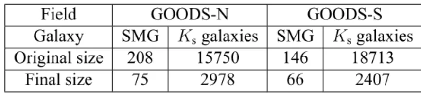
To perform cross-correlation analysis in the field, we need to apply the same selection mask for all populations regarded. For the correlation analysis, we require random catalogs of galaxies at random positions across the fields. GOODS fields contain several bright stars with large holes, where very few galaxies are detected in the catalogs. We create a mask according to it, and apply the mask to random catalogs, SMGs, and the K_s galaxies so that the positions of the random galaxies would be unbiased with respect to the SMG and K_sgalaxy samples, thus the correlation analysis would be unaffected by the holes. The final images are as shown in Fig. 2.6 on page 15, with an area∼ 100 arcmin² (radius∼ 6^′). The resulting GOODS-N photometric catalog comprises a total of 2978 sources while 12% have z_spec , and GOODS-S comprises 2407 sources while 20% have z_spec. Furthermore, SMGs sample have reduced to 75 and 66 in GOODS-N and GOODS-S, respectively. We summarize the number of galaxies used in Table 2.1.

Field GOODS-N GOODS-S

Galaxy SMG K_sgalaxies SMG K_sgalaxies

Original size 208 15750 146 18713

Final size 75 2978 66 2407

Table 2.1: Galaxy samples used in this study. We choose SMGs with S850 > 2mJy and σ < 0.5mJy.

Infrared Ksnormal galaxies (5σ) are chosen to reside in the same area coverage, with 1 < z < 3.

(35)

Figure 2.6: (a) GOODS-N (b) GOODS-S

Two-dimensional distribution of SMGs and infrared normal K_sgalaxies in GOODS fields that are used in our analysis. The SMGs shown represent the subset of the full samples SMGs that have matched the noise and threshold cut. The Ksgalaxies are chosen to reside at z = 1−3 with 5 σ detection. The SMGs are shown here individually with red circles while galaxies are in gray points. The blank areas represent the regions which are excluded from the analysis, i.e., around bright stars where few galaxies have been detected.

(36)

(37)

Chapter 3 Correlation Analysis

In this section, we outline our methods for measuring the angular cross-correlation between SMGs and galaxies, the autocorrelation of the galaxies, the absolute bias and characteristic DM halo mass.

3.1 Correlation Method

To analyze the clustering properties of galaxy populations, we evaluate the two-point correlation function. The two-point correlation function can be measured by counting the number of unique galaxy pairs as a function of separation and comparing the resulting distribution to that of a catalog of random points with the same number density and subject to the same observing geometry. Because we detect galaxies on a two-dimensional surface, we use the angular correlation function, a projection of the three-dimensional spatial correlation function (Peebles 1980). The two-point correlation function provides us a robust way of tracing the dependence of large-scale structure on galaxy properties and evolution through redshift. Several estimators for the angular two-point correlation functions are available, we use the Landy and Szalay (1993) estimator for observed angular correla- tion function ( hereafter ω_obs), which have shown to have minimum variance and bias, as described by

ωobs(θ) = DD(θ)− 2DR(θ) + RR(θ)

RR(θ) , (3.1)

(38)

where DD(θ), DR(θ) and RR(θ) are the galaxy-galaxy, galaxy-random and random- random normalized pair counts, respectively.

However, since the angular correlation is the excess probability of finding a data pair versus finding a random pair, as the data pairs decrease over distance the normalized number of random pairs is greater than the number of data pairs, ω_obs cannot be positive for all θ. Therefore, in field of finite size, estimators of the correlation function based on pair counts are subject to the integral constraint, which can be expressed as (Groth and Peebles 1977)

∫ ∫

ωobs(θ12) dΩ1dΩ2 ≃ 0, (3.2)

where θ₁₂ is the angle between the solid angle elements dΩ₁ and dΩ₁ and the integrals are over the survey area. The size of this bias increases with the clustering strength and decreases with field size; in our very small field studies, it is a significant effect and a correction must be made. The integral constraint correction is approximately constant and equal to the fractional variance of galaxy counts in a field,

IC≈ 1

⟨Ngal⟩ + ω_Ω, (3.3)

where the first term on the right is the Poisson variance and the second accounts for the additional variance caused by clustering (Peebles 1980),

ω_Ω = 1 Ω²

∫ ∫

ω(θ₁₂)dΩ₁dΩ₂, (3.4)

In this study we consider the latter term ωΩonly since it dominates the integral constraint.

ω_Ω is dependent on the intrinsic clustering of galaxies, normally by adopting some form for ω(θ). We use the formalism of Roche and Eales (1999),

ω_Ω =

∑RR(θ)ω(θ)

∑RR(θ) . (3.5)

Numerous studies have shown that most galaxy populations obey power law approx-

(39)

imation on the angular correlation function ( hereafter ACF ),

ω(θ) = A ( θ

1 rad )_−δ

. (3.6)

Adopting power law form of ACF, the resulting correlation returns

ω_obs = A (

θ^−δ −

∑RR(θ)θ^−δ

∑RR(θ) )

. (3.7)

The second term in the bracket is the geometric feature of field studied, which we name C hereafter if mentioned. The uncertainty in the Landy and Szalay estimator can be estimated by assuming that DD(θ) has Poisson variance, in this case

σ_obs(θ) = 1 + ω(θ)

√DD(θ). (3.8)

Derive the ACF on small sample (number of SMG∼ 10²) is expected to produce very large statistical errors, reducing our ability to derive well-constrained clustering properties (Chen et al. 2016). However, we can apply a closely related correlation function: the two- point cross-correlation function (CCF), by using the larger sample of Ks-band selected galaxies in the same field. We cross-correlate the target sample galaxies (D_s) with the tracer galaxies (D_t), as follows:

ω_obs(θ) = D_sD_t(θ)− DsR(θ)− DtR(θ) + RR(θ)

RR(θ) , (3.9)

where both data sets are normalized by the total pair counts. By cross-correlating a small target sample (SMGs) with a large tracer population (K_s tracer galaxies, we explain the subset selection in next section), we significantly increase the number of pairs, reaching greatly reduced statistical uncertainties, compared to directly derive the ACF of SMGs alone.

(40)

3.2 Tracer Galaxy Subset

To understand the clustering feature of SMGs we first apply the ACF on Ksgalaxies.

The larger sample size enables us to derive the clustering properties from ACF alone. The galaxy autocorrelation varies with redshift, owing to the evolution of large-scale struc- ture. In our study we choose K_s galaxies with magnitude 24.5 > m_K_s > 19.5 with 5σ detection. This is done to remove galaxies with marginal flux detection that may arise due to false detection. This selection has been done in both GOODS fields. The use of flux-limited sample however means that we select more luminous galaxies in high red- shift regions. These fewer luminous high-z infrared galaxies will affect the correlation function between SMGs and K_sgalaxies since they dominate the CCF where SMGs are peaked at redshift space, but have tiny effect on ACF due to their small number, shallow the strength of CCF to interpret the SMGs clustering feature. To overcome the inconsis- tency and improve the reliability of the CCF calculation, we random choose K_s galaxies with redshift overlap with SMGs redshift distribution in each redshift bins to enter the correlation calculation, i.e., the tracer galaxies. We have made the assumption that SMGs and tracer galaxies follow the same galaxy evolution scheme. We use this smaller tracer galaxy sample to calculate the ACF and CCF. In our analysis we model about 2000 tracer galaxies in correlation calculation to maximize usage of high-z galaxies with replacement (see Fig. 3.1 on page 21).

3.3 Uncertainties of ACF and CCF

The subset usage for K_sgalaxies however means that we lose information on other galaxies excluded. The ACF result alters when we choose different tracers to enter the calculation. We employ an iteration method to minimize this effect. Firstly, we choose a tracer subset and do bootstrap resampling to give correlation function and error. Secondly, the process is iterated until the spread in correlation function in single angle bin converges and dominants over the Poisson errors, therefore we combine all measurements to obtain the mean and the uncertainty. The same strategy has been applied on CCF calculation.

(41)

Figure 3.1: Redshift distributions for the Ksgalaxy sample in the redshift range z = 1−3 (solid green line), and the SMG redshift distribution in the range z = 1−4 (dotted red line). The histograms for all populations have been scaled so that the distribution can be directly compared to each others. Also shown is the redshift distribution for tracer galaxies (dashed blue line) selected to match the overlap in the redshift distributions of the SMGs, as used in both ACF and CCF analysis. 12% in GOODS-N and 20% in GOODS-S galaxies have spectroscopic redshifts. We use z_specif any, otherwise z_photois used instead.

(42)

The random catalogs used are always 10 times larger than the tracers throughout the whole work.

3.4 Galaxy Bias

According to the current cosmological paradigm of structure formation, galaxies form and evolve inside dark matter halos (White and Rees 1978). In other words, there exists a connection between the DM distribution and galaxies in the dense DM regions.

The galaxy spatial distribution, however, is linearly biased with respect to the DM density field. The strength of this effect is referred to as galaxy bias, or bias in common. In prac- tice, there are two ways to obtain the bias: power law method and HOD modeling. We use power law method in this study and leave HOD modeling for further discussion. One of the simplest way to obtain bias is from the large-scale angular correlation analysis. The linear scaling gives the relative bias between two galaxy types,

b²₁₂= ω_gal1,gal2 ωDM

, (3.10)

where 1,2 represent types of galaxy, numerator the correlation function between two populations and denominator the dark matter correlation function if we assume two populations trace the same DM distribution ( or DM halo mass function ). Note that it reduces to absolute bias if we use the autocorrelation function in the numerator.

The mass of the DM halos in which K_sgalaxies and SMGs reside are reflected in their absolute clustering biases relative to the DM distribution, b_tand b_srelatively. To estimate DM halo mass of SMGs, we calculate the relative bias between SMGs and K_sgalaxies, b_st from which we derive the absolute bias of SMGs relative to DM, b_s. To determine absolute bias (following Ichikawa et al. 2007, Myers et al. 2007, Hickox et al. 2011), we first calculate the two-point autocorrelation of DM as a function of redshift. We use the HALOFIT code of Smith et al. (2003) to determine the nonlinear-dimensionless power spectrum ∆²_NL(k, z) of the DM assuming our standard cosmology, and the slope of the initial fluctuation power spectrum, Γ = Ω_mh = 0.21. We then project the power spectrum

(43)

∆²_NL(k, z) into the angular correlation, as shown Equation (A6) in Myers et al. (2006). The key parameter is the redshift distribution of the galaxies (SMGs and K_sgalaxies), which we have assumed to be the same in our analysis (see Section 3.2 and Fig. 3.1 on page 21),

dN_SMG

dz = dN_K_s

dz . (3.11)

For each correlation analysis we fit the correlation value to the DM ω_DM(θ) by minimizing χ²with linear scaling, as shown in Equation (3.5). This linear scaling ratio yields b²_t for K_s galaxy ACF or b²_stfor SMG-Ksgalaxy CCF. Finally, we use btand bstto infer the absolute bias of SMGs in the fields through

b_s = b²_st bt

. (3.12)

With this linear bias b_swe infer the expected ACF of SMGs by multiplying out the tracer population bias from the CCF by b²_st/b²_t or b_s/b_t, allowing us to compare the ACF of all populations.

3.5 Clustering Length r

₀

3.5.1 Power Law Model: Limber’s Equation to Clustering Length r

_0,SS

When the correlation function is expressed in power law model (default if no additional subscript), the spatial correlation function can be written as (Peebles 1980; Myers et al. 2006)

ξ(r, z) = [r

r₀ ]_−γ

, (3.13)

where γ is the power law slope, r₀ is the spatial clustering length if we assume no evolution with redshift in the clustering of the sample. The spatial correlation function can be integrated to yield its angular projection,

ω(θ) = A ( θ

1 rad )_−δ

. (3.14)

(44)

In the small angle approximation, we can invert Limber’s equation as

δ = γ− 1 (3.15)

A = H_γ

∫_∞

0 (dN₁/dz)(dN₂/dz)E_zχ¹^−γdz [∫_∞

0 (dN₁/dz)dz] [∫_∞

0 (dN₂/dz)dz]r^γ₀, (3.16) where H_γ = Γ(0.5)Γ(0.5 [γ− 1])/Γ(0.5γ), Γ is the gamma function, χ is the angular comoving distance, dN_1,2/dz are the redshift distributions of the samples, E_z = H_z/c = dz/dχ. The Hubble parameter H_z can be found via

H_z² = H₀²[

Ω_m(1 + z)³+ Ω_Λ]

. (3.17)

In our analysis we have chosen flat cosmology, therefore χ reduces to the radial comoving distance. Note that dN₁

dz = dN₂

dz in the ACF. Owing to the small size of SMGs which can hardly provide significant constraint on both the slope δ, or γ and the clustering amplitude A, we simply assume γ = 1.8 in analysis (e.g., Quadri et al. 2007 for ACF; Hickox et al.

2012 for CCF). We fit power law with integral constraint correction to the correlation functions using the expression above (see Equation 3.3), derive the corresponding r_{0, SG}, r_{0, GG} and r_{0, SS}.

3.5.2 Linear Growth Perturbation Theory (L): Large-scale Galaxy Bias to SMG r

0,SS,L

Differ from the previous section, we use the evolution of large-scale mass fluctuation (with subscript L) in linear regime to determine the correlation length of SMG, r_0,SS,L.(e.g., Lindsay et al. 2014; Durkalec et al. 2015). σRis the mass fluctuation in a comoving sphere of scale radius R h⁻¹Mpc. Following the galaxy bias definition, we have

σ_R,g(z) = b_L(M, z)σ_R,m(z), (3.18)

where bL is the galaxy bias. The usually adopted value for σ is R = 8 h⁻¹ Mpc and in this work we use σ_8,m(z = 0) = σ₈ = 0.84. In the model the redshift evolution of mass

(45)

fluctuation is described as

σ8,m(z) = σ8,m(z = 0)D(z), (3.19)

where

D(z) = g(z)

g(0)(1 + z), (3.20)

and g(z) is the normalized growth factor, which describes how fast the linear perturbations grow inside with the scale factor. We write

g(z) = 5 2Ωmz

[

Ω^4/7_mz − ΩΛz+ (

1 + Ω_mz 2

) (

1 + Ω_Λz 70

)]₋₁

, (3.21)

(Carroll et al. 1992) and the cosmological parameters evolves in a flat cosmology as

Ω_mz = (H0

H_z )2

Ω_m(1 + z)³ Ω_Λz = (H0

H_z )2

Ω_Λ. (3.22)

Since σ_8,gis the clustering strength of halos more massive than stellar mass M at redshift z, following Peebles (1980)

σ_8,g=

√ C_γ

( r₀

8 h⁻¹ Mpc )γ

, (3.23)

with

C_γ = 72

2^γ(3− γ)(4 − γ)(6 − γ), (3.24)

where γ is the power law slope. We can retrieve correlation length r₀as follows:

r₀ = 8

(b_Lσ₈D(z) Cγ

)¹

γ

, (3.25)

when we use fixed value of γ = 1.8 to imply the derived absolute bias of SMG at its median redshift to obtain the r_0,SS,L.

(46)

3.5.3 Difference Between Power Law Model and Linear Growth Per- turbation Theory (L)

Two-point correlation functions have been widely used in studying the clustering phenomena of different galaxy populations. Following Peebles (1980), numerous works have suggested that stellar populations obey the simple power law model. In this work, the presumed hypothesis is that CCF can be used to infer SMG ACF and to derive the clustering parameters.

For the power law method, we estimate observed clustering length r_0,SSby measuring the correlation amplitude and absolute bias b_sby fitting the observed correlation function to the DM distribution (following Hickox et al. 2011). We obtain CCF b_st and A_st from observation then derive b_sand A_sof SMG accordingly. Firstly, to better utilize this method depends largely on the data quality, i.e., sample sizes, field of view, luminosity, catalog completeness etc. In this study we have very small sample sizes (SMG∼ 10²) with the survey area of ∼ 6^′ × 6^′. We obtain reasonable result with acceptable error, however this result can be doubtful due to data deficiency, which may induce unavoidable Poisson noise into the calculation, as described in the Section 3.1. Secondly, the details within the redshift distribution of populations and DM are required to obtain b_t/ b_st/ b_s, strictly restricting ACF and CCF to stick to DM-like distribution, which is only true in large-scale.

Finally, SMG ACF is forced to follow power law model to derive the r_0,SS, and this could lead to abnormal result if the power law model is poorly constrained on the correlation function.

On the other way around, linear growth perturbation theory can predict the large-scale evolution of mass fluctuation. We can estimate the large-scale galaxy bias b_L where the target population resides in at particular redshift, should we hold the accurate cosmological parameters and the observed clustering strength of the population. We can invert the relation to obtain r_0,SS,Lif we get the large-scale galaxy bias b_L. We use b_L = b_s, meaning that the derived absolute bias of SMG in our study equals to the large-scale galaxy bias predicted in the linear growth regime at the ¯z = 2.5. This however is an approximated scenario only because of our small field size. The real large-scale bias could possibly be

(47)

smaller in our case, where we try to infer the observed clustering strength r_0,SS,Lby partly assuring the appropriateness to use large-scale bias.

These two methods should return similar correlation results when sufficient data in large-scale are included. We hereafter estimate the corresponding clustering length and derive the DM halo mass.

3.6 Dark Matter Halo Mass

To simplified the analysis, we use a bias-halo mass relation published by Sheth et al.

(2001). They derived a relation between DM halo mass and large-scale bias that agrees well with the results of cosmological simulations. We use the formalism of Sheth et al.

(2001) to convert b_s to M_halo at the mean redshift (z ∼ 2.5). This characteristic Mhalo

corresponds to the top-hat virial mass (Peebles 1993, and references therein), in the simplified case in which all objects in a given sample reside in halos of the same mass. This assumption is justified by the fact that SMGs have a very small number density compared to the population of similarly clustered DM halos (in our case the tracer galaxies), such that it is reasonable that SMGs may occupy halos in a relatively narrow range in mass. It is worth noting that we have assumed the biases we use to derive the DM halo mass are the large-scale bias of galaxies. We explain the discrepancy further in Section 4.6.

(48)

(49)

Chapter 4 Results and Discussions

In this section we discuss the results of the correlation analysis and the derived spatial clustering length r0.

4.1 K

_s

Galaxy ACF

We calculate the ACF of K_sgalaxies for each GOODS field. The geometric feature factor C (the last term in Equation 3.7) are similar in both fields, differs only 11 %. To conduct cross-field comparison, we use the average value of ¯C throughout correlation calculation. This ¯C term originated from integral constraint (IC) has a significant effect at large angle separation, and IC causes the measured correlation to decay to negative at θ > 100^′′, which is inappropriate for analysis. The tracers, K_s-selected galaxies have a positional uncertainty within 1^′′ radius. Therefore we choose the interval between 2^′′ ≤ θ≤ 100^′′ for our interest.

The observed ACF is significant on the scales from 2^′′ to 100^′′ (see Fig. 4.1 on page 30), and the best-fit slopes are

γ_N= 1.87± 0.24 γ_S= 1.75± 0.07,

where N and S represent GOODS-N and GOODS-S, respectively. Within the 1σ signif-

(50)

Figure 4.1: The ACF of Ks-selected normal galaxies in the GOODS fields.

Galaxies are selected to match the overlap of the SMGs and galaxies in redshift space. Uncertainties are estimated from standard deviation of the bootstrap resampling result. The ACF of DM evaluated for the redshift distribution of the galaxies is shown by the dashed black line. The power law fit is performed on scales of 2^′′–100^′′ and is shown as the solid lines. The green solid line is the best-fit power law model with the integral constraint (IC, consists of geometric factor ¯C) correction while red line is the one without correction. To reduce the downsizing amplitude effect arises from small survey area, we consider angle separation smaller than 100^′′. The observed amplitude of the Ksgalaxy ACF yields the absolute bias bt, which we use to obtain the absolute bias bsand DM halo mass of the SMGs.

(51)

icance they agree well with the literature value of γ = 1.8 (e.g., Peebles 1980; Roche and Eales 1999; Coil et al. 2008; Quadri et al. 2007; Ichikawa et al. (2007); Zehavi et al.

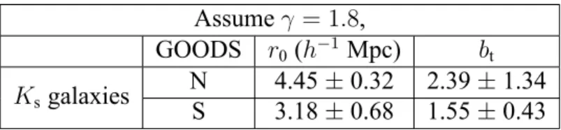
2011), so we hereafter use this fixed value unless specified. The derived spatial clustering length r0,GGwith γ = 1.8 gives

r_0,GG,N= 4.45± 0.32 h⁻¹Mpc r0,GG,S= 3.18± 0.68 h⁻¹Mpc.

These values are comparable with previous studies in the fields, i.e., Quadri et al. (2007), Ichikawa et al. (2007) on GOODS-N K-selected galaxy catalog (flux limited sample, high redshift) with r_0,GG,N ∼ 4.8−6.0 h⁻¹Mpc; Hickox et al. (2012) on ECDFS IRAC galaxies with r0,GG,S = 3.3± 0.3 h⁻¹Mpc. We summarized our results in Table 4.1.

The main difference between our work and the previous studies is that we do not include redshift information in the calculation of correlation function. Redshift PDF rep- resents the uncertainty in the redshift estimation due to the observational limitation, so by introducing the redshift PDFs as the weighting in the correlation method (e.g. Myers et al.

2009), one accounts all the possibilities that the target resides in redshift space. Instead of treating redshift PDFs as the statistical interpretation of observational limitation, we treat all galaxies as point targets within the redshift space. During our calculation we use the single z_photo or z_specas the accurate redshift, intending to approach the clustering features obtained in the literature. Our result provides a first glance on the methodology applica- tion on this study, i.e., the use of accurate redshift PDF in correlation is not necessary to achieve acceptable and similar results.

Assume γ = 1.8,

GOODS r₀(h⁻¹Mpc) b_t K_sgalaxies N 4.45± 0.32 2.39± 1.34

S 3.18± 0.68 1.55± 0.43

Table 4.1: Result of Ks-selected near-infrared normal galaxies ACF.