合歡山地區台灣高山田鼠(Microtus kikuchii)排遺對土壤氮的影響

國立臺灣大學生命科學學院生態學與演化生物學研究所 碩士論文

Institute of Ecology and Evolution Biology College of Life Science

National Taiwan University Master Thesis

合歡山地區台灣高山田鼠(Microtus kikuchii) 排遺對土壤氮的影響

Effects of Taiwan vole (Microtus kikuchii) feces on soil nitrogen at the He-huan area

許元俊 Yuan-chun Hsu

指導教授：林雨德 博士 王巧萍 博士 Advisor: Yu-Teh K. Lin, Ph.D.

Chiao-Ping Wang, Ph.D.

中華民國 100 年 2 月

February, 2011

謝誌 謝誌 謝誌 謝誌

從第一次上山幫忙學姐做實驗時，感覺工作相當的辛苦難受，到後來反而覺得 上山做實驗，某種形式上來說是在渡假，回想起來覺得相當的有趣；要感謝林雨 德老師提供我研究的方向與支持，讓我有這個機會認識合歡山、與田鼠邂逅以及 徜徉在高山草原之間，除此之外，不遲辛勞的在我碩士生涯中對我的鞭策及指導。

也要感謝我的共同指導老師-王巧萍博士，對我這個只懂土壤學皮毛中的皮毛的學 生耐心的指導，還提供我實驗上所需的人力、物力；有以上兩位老師的指導，這 個論文才得以完成。還要感謝口試委員：陳尊賢老師及林登秋老師對論文的建議。

感謝特有生物中心高海拔試驗站的林旭宏主任、艾台霖大哥、張錫樑大哥、蔡 銘源大哥及小青姐，讓我們在合歡山可以有一個溫暖、自在的休息空間。感謝實 驗室的淑蕙學姐、壽嶽學長、婷婷學姐、菡芝、育欣、嚕嚕米、土匪、徵葳、瀅 淳、艾陵、威廷、胖達、友志、允光，為實驗室帶歡樂，而且在實驗上或生活上 對我提供的幫忙與支持；菁羚、素含及呱呱華更是在山上一起為實驗奮戰的好夥 伴，還能讓大家吃到好料，有你們在真好！感謝林試所土壤實驗室的助理馨薇、

仙貝、素媚、莉莉、佳雯，在實驗上的幫忙，尤其是馨薇，沒有你教我使用儀器 及實驗方法，我的實驗真的是不用做了。還要感謝小怪學長及璽全學長，願意當 小幫手來協助實驗，沒有你們的幫忙實驗進行上會相當的困難。還有台大土調研 究室的君至學姐與治懿學姐，在實驗早期給我許多資源與協助，讓我可以對於土 壤方面比較進入狀況。

謝謝我爸爸、媽媽在這段時間不過問的支持，讓我可以自由自在的渡過研究生 涯；謝謝陪伴我的朋友們，可以聽聽我的抱怨，或是帶我出去玩樂，幫我化解在 研究上遇到的怨念；還要謝謝生科系籃的各位，對我的包容與尊重，讓我在這個 團隊裡充滿了歸屬感，更是支持我的動力。最後謝謝高山田鼠們，沒有你們也就 沒有這個實驗，但也要向所有因實驗而不幸犧牲的動物們說聲抱歉。

摘要 摘要 摘要 摘要

草食性動物取食植物，排出氮含量高且分解快的排遺，可以快速的將養分回 歸到土壤，提供氮一個快速循環的途徑(fast cycle)，進而影響植物的生長與群聚的 組成。大型草食性動物在生態系營養循環的作用已經有相當多的研究，但小型哺 乳動物所扮演的角色相關研究較少。台灣高山田鼠(Microtus kikuchii)為草食性小型 囓齒動物，在玉山箭竹草原中，族群數量多而穩定，並有排遺集中形成「公廁」

的習性。本研究想了田鼠排遺對高山草原土壤氮含量的影響，探討以下問題：(1) 高山田鼠的氮輸出量；(2)高山田鼠公廁的分佈及動態；(3)高山田鼠公廁對土壤氮 含量的影響；(4)田鼠排遺對植物凋落物分解的影響。我於 2007 年起在合歡山的玉 山箭竹草原中進行田鼠族群及野外公廁調查，透過飼養來計算田鼠排遺量，並在 實驗室與野外進行田鼠公廁的孵育實驗。結果顯示，田鼠的氮輸出量範圍在 0.33 ~

0.41 kg N ha^-1 year^-1；高山田鼠族群及公廁分佈具空間異質性，公廁數目大抵隨田

鼠族群數目波動，對土壤氮時空分佈影響很大；公廁會增加土壤中可萃取性氮，

尤其是植物可利用的無機態氮；公廁易分解的養分主要在一個月內釋出，對土壤 的有效供應期限約為 1 個月；田鼠排遺提供土壤微生物較易取得的食物資源而使 其活性增加，加速土壤有機質的分解，微生物扮演的角色尚須進一步的研究以了 解。綜合而言，在土壤有機質含量很高，但是分解緩慢的高山生態系，田鼠公廁 不僅提供養分，並能加速原來土壤中的有機質分解，對高山生態系而言，扮演相 當重要的角色。

關鍵字：台灣高山田鼠、排遺、公廁、氮循環、分解

Abstract

Herbivore returns nitrogen to soil by defecating high-nitrogen wastes. The fast

decomposition rates of feces provide a “fast cycle” for returning plant nitrogen to soil.

The temporal production and spatial distribution of feces can affect the dynamics of

nutrient availability in soil, and change plant community structures. The effects of feces

were well-documented for large herbivores, but not herbivorous small mammals. The

Taiwan vole (Microtus kikuchii) is the dominant herbivorous rodent in alpine meadow

in Taiwan. They deposit large amount of feces at latrine sites. I want to investigate the

effects of latrines on soil nitrogen. This thesis is divided into four aspects: (1) Nitrogen

output of vole; (2) The temporal dynamics of vole latrines; (3) The effects of latrines on

soil nitrogen; (4) The effects of latrines on plant litter decomposition. I conducted vole

and latrine survey starting in 2007 at an alpine meadow in He-huan Mountain. Nitrogen

output was acquired by rearing voles in the laboratory. I also conducted two field and

one laboratory incubation experiments with latrines. The results showed that, annual

nitrogen output of voles was 0.33~0.41 kg N ha^-1 year^-1. Vole latrines increased the

extractable nitrogen in soil, especially inorganic nitrogen. The release of nutrients from

liable part of feces to soil occurred within one month. Latrines also provided liable

carbon to microbes, increasing microbial activities and decomposition rates of soil

organic matters. The spatial patterns of vole and latrine abundances were highly

heterogeneous in alpine meadow. The temporal dynamics of voles and latrines further

increased the spatial heterogeneity of soil nitrogen. Alpine meadows had high soil

organic matters, yet decomposition rates were low. Vole latrines not only quickly return

nutrients back to soil, but also enhance decomposition rates of soil organic matters, thus

play a crucial role in alpine ecosystems.

Keyword: decomposition, feces, latrine, Microtus kikuchii, nitrogen cycling, Taiwan

voles

Content

謝誌 謝誌 謝誌

謝誌 ... i

摘要 摘要 摘要 摘要 ... ii

Abstract ... iii

Introduction ... 1

Research objectives ... 5

Materials and Methods ... 5

Study Site ... 5

Nitrogen Output by Taiwan Voles ... 7

Taiwan vole population survey ... 7

Daily defecation rates of voles ... 8

Vole Latrine Survey ... 9

Natural Latrines ... 10

Field Incubation on Natural Soil ... 11

Field Incubation on Homogenized Soil ... 12

Preparing soil ... 12

Experimental setup ... 13

Chemical analyses ... 14

Laboratory Incubation on Homogenized Soil ... 15

Preparing soil, feces, & plant litter ... 15

Experimental setup ... 15

Chemical analysis ... 19

Soil microbial biomass, extractable nitrogen, extractable carbon ... 19

C and N content ... 20

Organic matter content of soil ... 21

CO

evolution rate ... 22

Statistical Analyses ... 22

Results ... 23

Taiwan vole population survey ... 23

Daily defecation rates of voles ... 25

Nitrogen output of vole populations ... 26

Vole latrines survey... 28

Field Incubation on Natural Soil ... 29

Natural Latrine ... 30

Field Incubation on Homogenized Soil ... 31

Laboratory Incubation on Homogenized Soil ... 39

Discussions ... 53

Taiwan vole population survey ... 53

Daily defecation rate ... 54

Nitrogen output of vole ... 56

Vole latrine survey ... 58

Field incubation on natural soil ... 59

Field incubation on homogeneity soil ... 60

Appendix ... 72

Content of Tables

Table 1. The characteristics of soil from the study site at the He-huan Mt. ... 12 Table 2. Precipitation and air and soil temperature of study site at the He-huan Mt. .... 14 Table 3. The N and C output of vole feces ... 26 Table 4. The number of voles and latrines ... 29 Table 5. Statistic results of of field incubation on homogenized soil ... 34 Table 6. The proportions of extractable N and C to the total N and C in field incubation

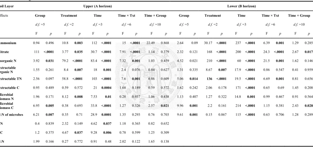
on homogeneous soil. ... 33 Table 7. Statistic results of laboratory incubation experiment. ... 40 Table 8. Initial chemical compositions of soil at in laboratory incubation. ... 49 Table 9. Statistic results of the effects of vole feces and plant litter on the N and C of

soil. ... 49 Table 10. Weight, N, and C content of fecal pellets and leaf litter ... 53

Content of Figures

Fig. 1. The soil-plant-animal relationship in grassland ecosystems ... 3

Fig. 2. Vole survey plot ... 7

Fig. 3.Vole density at each sampling plot ... 24

Fig. 4. Number of male and female voles at study site ... 24

Fig. 5. Daily defecation rates of voles in different month/year ... 25

Fig. 6. Nitrogen output of voles at different months ... 27

Fig. 7. Number of vole latrines per 100 m² in each plot. ... 27

Fig. 8. Frequency distribution of the number of fecal pellets in latrines ... 27

Fig. 9. The relationships between the number of voles and the number of latrines. ... 29

Fig. 10. The retention rate and number of new latrines occurred between surveys ... 29

Fig. 11. Nitrogen contents of soil at the study site. ... 30

Fig. 12. Nitrogen concentration of soil under natural vole latrine and control. ... 31

Fig. 13. Concentrations of ammonium, nitrate, and overall inorganic N in the soil extract of field incubation on homogenous soil ... 35

Fig. 14. Concentrations of extractable organic N, extractable total N, and extractable total carbon in the soil extract of field incubation on homogenous soil ... 36

Fig. 15. Concentrations of microbial biomass N and C, and C:N ratio in the soil extract of field incubation on homogenous soil ... 37

Fig. 16. Concentrations of TN and TC, C:N ratio, and organic material in the soil extract of field incubation on homogenous soil ... 38

Fig. 17. Percentage of initial weight remained in fecal pellets... 38

Fig. 18. C and N content, and C:N ratio in fecal pellets. ... 39

Fig. 19. Percentage of N and C remained in fecal pellets. ... 39

Fig. 20. N and C concentrations in leachate of control. ... 40

Fig. 21. The concentrations in leachates ... 41

Fig. 22. The concentrations difference between treatment and control ... 42

Fig. 23. The total amount accumulated in leachates ... 43

Fig. 24. The relative leaching rate of treatment than control ... 44

Fig. 25. CO₂ evolution rates ... 48

Fig. 26. Concentration of extractable C and N in soil at the end of incubation ... 50

Fig. 27. C and N of soil microbes and soil of labatory incubation ... 51

Fig. 28. Fecal pellets and leaf litter in single or mixed treatment after incubation ... 53

Introduction

In many terrestrial ecosystems, plant growth is nitrogen limited (Aerts and Chapin 2000). The main nitrogen used by plants is inorganic nitrogen (NH4+

& NO3-

). Yet, inorganic nitrogen content is usually very low in soil, and must be supplied from the mineralization of organic matters by microbes. Soil organic matter (SOM) is the largest nutrient reserve in grassland ecosystems. It contains more than 60% of C, N, and P within the ecosystem (Dubeux et al. 2007). Decomposition rate of SOM is affect by the quality of organic matters, content of lignin, N, P and C:N ratio, and the weather, temperature and moisture (Taylor et al. 1989, Semmartin et al. 2004). Factors that alter the quantity and quality of SOM can profoundly influence the nitrogen cycles in terrestrial ecosystems (Dubeux et al. 2006a, Dubeux et al. 2007).

Herbivores can have a strong impact on plants and environment in an ecosystem (Gibson 1989, Haynes and Williams 1993, Pastor et al. 1993, Sirotnak and Huntly 2000, Bakker and Olff 2003, Villarreal et al. 2008). Particularly, herbivores largely influence the quantity and quality of SOM, thus change the nitrogen turnover rate (Holland and Detling 1990, Pastor et al. 1993, Bakker et al. 2004, Semmartin et al. 2004, Fornara and Du Toit 2008). Over short term, herbivores remove standing vegetation, and contribute to litter buildup (Canals and Sebastia 2000, Bakker et al. 2004, Semmartin et al. 2004, Dubeux et al. 2006b, Fornara and Du Toit 2008). Herbivores also deposit high-nitrogen waste products (urine and feces). Furthermore, defoliation by herbivore grazing can quickly stimulate nitrogen uptake ability of roots (Seagle et al. 1992, Bardgett et al.

1998, Frost and Hunter 2007). The increased plant N content through herbivore grazing stimulation and animal excreta would decrease the C:N ratio of plants. The increased plant quality, in turn, could increase the quality of plant litter (Day and Detling 1990, Haynes and Williams 1993). High quality SOM has a faster decomposition rate, which

enhances nitrogen turnover (Holland and Detling 1990).

Over long term, soil disturbance (Inouye et al. 1987, Gibson 1989, Questad and Foster 2007, Villarreal et al. 2008) and selective foraging by herbivores could change plant community composition (Pastor et al. 1993, Sirotnak and Huntly 2000, Stark et al.

2002) thus SOM composition. For example, animal burrow can increase soil aeration.

Burrows also mix upper and lower layer soil, redistributing nutrients and bringing organic matter into soil, which stimulate microorganism activity (Inouye et al. 1987, Gibson 1989, Canals and Sebastia 2000). Herbivores often selectively forage on high-quality plants (low C:N ratio), decreasing the abundance of those plants (Pastor et al. 1993, Sirotnak and Huntly 2000), increasing the proportion of low quality litter, which in turn decreases mineralization rates (Pastor et al. 1993, Sirotnak and Huntly 2000).

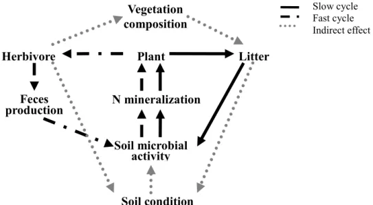
The nitrogen cycle in a grassland ecosystem could be described in a soil-plant-animal system (Fig. 1.) that has two sub-cycles (Haynes and Williams 1993, De Mazancourt et al. 1998, Bakker et al. 2004). In one sub-cycle, plants return nutrients to soil via litter. With slow turnover rates, most of the litter is added to the SOM compartment (Bardgett et al. 1998). Only part of the litter is decomposed, nutrients released and become readily available. It is named the slow cycle (Bardgett et al. 1998, Bakker et al. 2004). In the other sub-cycle, herbivores create a shortcut in the slow cycle by consuming plants. Herbivore wastes have a faster turnover rate, and contain more easily accessible nutrients, i.e., a fertilizer effect (Williams and Haynes 1995, Willott et al. 2000, Dubeux et al. 2007, Moe and Wegge 2008). It is name the fast cycle (Pastor et al. 1993, Bardgett et al. 1998, Bakker et al. 2004). In this research, I focused on investigating the effects of nitrogen return from feces, yet also examined the effects of feces on plant litter decomposition.

Fig. 1. The soil-plant-animal relationship in grassland ecosystems as adopted from Bakker et al. (2004).

Herbivores can return a large amount of nitrogen to soil via feces, e.g., cattle 1.3~4.7 kg ha^-1 yr^-1 (Schimel et al. 1986) and elk 4.9~45.6 kg ha^-1 year^-1(Singer and Schoenecker 2003)(Frank et al. 2000). Nitrogen released from feces can create high nutrient concentration localized patches (Afzal and Adams 1992, Haynes and Williams 1993, Williams and Haynes 1995, Lovell and Jarvis 1996). For example, Willott et al.

(2000) found that rabbit latrine increased 2-fold organic carbon concentration and 4-fold inorganic nitrogen concentration in soil beneath latrines, and decreased more than 30%

root:shoot ratio of barley in laboratory culture experiment with latrine. Feeley (2005) also found that howler monkey latrine form a “fertile island” with increased 2~3-fold nitrogen concentration and 2~4-fold phosphate concentration in the soil.

Plants can quickly pick up nitrogen from feces, as supported by using stable isotope ¹⁵N (Cochran et al. 2000, Frost and Hunter 2007). Not only do herbivore’s feces have fertilizer effect but also carnivore’s. River otter feed on high δ¹⁵N value food (intertidal fish and invertebrates) and then feces had higher δ¹⁵N value than plants (Ben-David et al. 1998). Plants growing in latrine site had higher δ¹⁵N value than no latrine site. River otter transport N & P from water-to-land at latrine site supplying

Slow cycle Fast cycle Indirect effect

Herbivore Plant Litter

Vegetation composition

N mineralization

Soil microbial activity

Soil condition Feces

production

Ben-David 2007).

Feces also contain a large amount of carbon. The amount of carbon released is often greater than that of nitrogen during decomposition (Pastor et al. 1993, Pastor et al.

1996). When SOM is high in soil, the readily available carbon may be very low (Hatch et al. 2000). Animal feces add fresh labile carbon to the soil, and can promote an increase in the biomass and activity of soil microbes (Afzal and Adams 1992, Williams and Haynes 1995, Cochran et al. 2000, Frank et al. 2000, Hatch et al. 2000). Several studies found that after animal dung were deposited, microbial biomass and activity were increased, but adding fertilizer N could not elicit the same response (Lovell and Jarvis 1996, Hatch et al. 2000). Feces can elicit more nutrient mineralization in soil.

Pastor et al. (1993) found soil incubation with intact moose fecal pellet on it could mineralize more carbon and nitrogen than combining the mineralized amount of moose fecal pellet and soil incubation separately.

Most researches of feces fertilization focused on large herbivores, especially ungulates and cattle. Few focused on small herbivores. According to previous research, however, small herbivores could provide similar amount of nitrogen from feces as large herbivores. Clark et al. (2005) estimated annual nitrogen output from fecal, urinary, and total nitrogen by small mammals in Center for Subsurface and Ecological Assessment Research (CSEAR), 1.00 (0.91~1.05), 2.75 (2.55~2.95), and 3.73 (3.46~3.99) kg N ha^-1 year^-1, respectively. Bakker et al. (2004) found after excluding large herbivore (cow) small herbivores (vole) return more N to soil through feces than large herbivores (cow) do. Pastor et al. (1996) found the potential mineralizable nitrogen in voles feces of Minnesota was 0.16 kg N ha^-1 year^-1. Although the nitrogen from feces was much lower, the value was still higher than the moose on Isle Royale (0.006 kg N ha^-1 year^-1). The vole’s feces also had a faster decomposition rate than moose (vole, k = 0.69~1.73;

moose, k =0.025~0.191). The great high turnover rates of nutrients in small mammals’

feces may affect seasonal availability of nutrients, although the amount was a very small portion of overall annual nutrient budgets of ecosystem.

Taiwan voles (Microtus kikuchii) often deposit large amounts of fecal pellets at the same sites, and form “latrines”. Latrines are easily observable in the field. At the alpine meadows of the He-huan Mt., large- or medium-sized herbivores are scarce (吳 2004), the Taiwan vole is the most dominant small herbivore (Ho 2009). It provides a good opportunity for studying the effects of small herbivore feces on the N cycling of alpine ecosystems.

Research objectives

I aimed to reveal the effects of Taiwan vole’s latrine on soil nitrogen in an alpine meadow. I focus on two questions. First, whether latrine can increase soil nitrogen content? Second, whether latrine can increase the decomposition rate of plant litter?

I approached the questions by measuring feces output of voles and nitrogen content of fecal pellets in the laboratory, and by monitoring the temporal and spatial dynamics of vole latrines. I created artificial latrines to perform field and laboratory incubation experiments.

Materials and Methods

Study Site

The study site was located at the He-huan Mountains (24°08’36.4”N,

121°17’17.4”E), ~ 3000 m in altitude, Nantou County, in central Taiwan. It was near the

western boundary of the Taroko National Park. Mean annual temperature was 7.0 ℃,

and mean annual rainfall 3,500 mm based on weather information collected at the

High-Altitude Station of the Institute for the Endemic Species Research, 5 km from our

study site. The weather could be divided into wet (May ~ October) and dry (November

~ April) seasons, with sporadic snow during January to March.

The study site was an alpine meadow on a 30~45° slope facing east, surrounded

by fir forests (composited of Abies kawakamii & Tsuga formosana). Yushan cane

(Yushania niitakayamensis), alpine silver grass (Miscanthus sinensis), and Carex spp.

were the three dominant plant species in the meadow. The local plant community was

described in details by Ho (2009). The soil was acidic (pH 3.3 in CaCl2), and described

as “Typic Haplumbrept, fine, illitic, frigid” (King 1993).

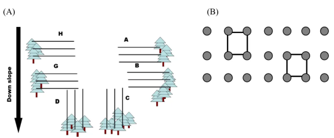
Two Taiwan vole survey plots were set up at upper (plot A, H), middle (plot B, G),

and lower (plot C, D) sections of the slope each (Fig. 3A) on October 2005 for a

plant-vole interaction experiment (Ho 2009). The six sampling plots were at least 200

meters apart from each other. Each plot had three parallel trap lines ran perpendicular to

the tree line jointing meadow and surrounding forest. Each line had seven trap stations,

and formed a 7 × 3 trapping grid in each plot (Fig. 3). Trap lines and trap stations within

each plot were 10 m apart.

(A) (B)

Fig. 2. (A) The six Taiwan vole survey plots on the slope of an alpine meadow. Each plot had three parallel trap lines ran perpendicular to the tree line jointing meadow and forest. The six plots were at least 200 meters from each other. (B) Each trap line had seven trap stations (solid circle). Trap lines and trap stations within each plot were 10 m apart. Two 10 × 10 m quadrats within the trapping grid were randomly selected to conduct latrine survey.

Nitrogen Output by Taiwan Voles

I used the methodology described in Clark et al. (2005) to estimate the nitrogen

output of voles. I measured nitrogen contents of fecal pellets, and daily defecation rates

of Taiwan voles. I also monitored vole population and latrine population dynamics.

Taiwan vole population survey

I conducted a population survey every two months from July 2007 to May 2009,

except during the snowy season (December–February), to estimate the population sizes

of Taiwan voles using the capture-mark-recapture method. The survey was a

continuation of a plant-vole interaction experiment starting in October 2005 (Ho 2009).

An Ugglan special live trap (250 × 78 × 65 mm) was placed at each trapping station.

Each trap was baited with rolled oats mixed with peanut butter, provided with a ball of

shredded newspaper for warmth. During each trapping session, traps were checked

twice daily at dawn (07:00~10:00) and nightfall (15:30~17:30) for three consecutive

nights, with a total of 6 trap checks. When voles were captured, each individual was

given a unique toe-clip for future identification. The following information of each

individual was recorded: trap station, species, toe-clip ID, sex, reproductive condition

(testes scrotal or abdominal for males; vagina perforated or non-perforated, and signs of

pregnancy and nursing for females), health condition (occurrence of parasites and scars),

and body weight. Animals were then released immediately at the station where they

were captured. I added 15 m buffer zone to each side of trapping grid to calculate the

effective trapping area which came to be 50 × 90 m². I applied the Pradel model in

Program MARK (Cooch and White 2010) to estimate vole population abundance, and

divided the value by 4500 m² to calculate density.

Daily defecation rates of voles

Five adult Taiwan voles of each sex (weighed ≧ 28 g, pregnant females were

excluded) were captured from an alpine meadow near the study site, brought back to the

laboratory in the High-Altitude Station in July 2007, March 2008, April 2009, and

January 2010. They were housed individually in standard rat cages (L×W×H: 40 × 25 ×

12 cm), with 3-inch thick wood shaving bedding, maintained in a light regime similar to

the wild, and provided with fresh Yushan cane (Y. niitakayamensis) leaves and water ad

libitum. (Ho 2009, Yeh 2010). Voles were maintained in such an environment for at

least 12 hours before the fecal pellets collection trials started. Each vole was then

weighed, and moved into a clear standard rat cage with 1 cm mesh wire at the bottom (a

collecting cage). Water and fresh Yushan cane leaves were provided ad libitum for 24

hours. At the end of trial, voles were removed from cages, and released back to alpine

meadow. I collected and weighted all fecal pellets (fresh weights) in the collecting cage.

A small portion of each fecal sample was dried at 65℃ for 48 hours. Samples were then

finely ground to analyze carbon and nitrogen contents. The rest of fresh fecal samples

were stored in a -20 ℃ freezer, and later used in the field and laboratory incubation

experiments.

Vole Latrine Survey

I randomly selected two 10 × 10 m quadrats within the trapping grid in each plot

to conduct latrine survey (Fig. 3B). The survey period was conducted accompanying

vole population survey (bimonthly, except January) during July 2007 to July 2008,

except that plot G and H were not surveyed until September 2007. There were total of

six surveys (5 in plot G and H). A vole latrine was arbitrarily defined as any vole fecal

pile with more than 10 fecal pellets. Each latrine was marked with a flag with a unique

ID. I recorded the ID, location, and number of fecal pellets of each latrine during survey.

I also graded the conditions by the % of a latrine that became disintegrated, whiten, or

molded. I estimated the abundance, recruitment rate, and persistent rate of latrines at

each plot using the Pradel model in Program MARK (Cooch and White 2010).

Natural Latrines

At July and September 07, I searched 5 vole latrines at the field in the same

meadow of defecation rate experiment. I collected soil samples (a 10-cm diameter ×

15-cm deep) beneath vole latrine and a random 1 m far paired control. I also collected

the new leave of Yushan cane near each soil sampling site. Soil samples were divided

into two parts: 0–5 cm and 5–15 cm in depth. I took approximately 150 g from each part,

and passed them through a sieve (mesh no: 3’/2, 5.66 m/m). 10 g of each sample was

treated with 100 ml 2 N KCl solution at 160 rpm/min for 1 hour in an orbital shaker.

The extractant was filtered with Whatman No.1 filter paper (11 µm). The filtrate was

then analyzed by the Kjeldahl Distillation Apparatus to estimate the amount of

extractable inorganic nitrogen, and extractable ammonium. I then calculate extractable

nitrate by subtracting extractable ammonium from extractable inorganic nitrogen. The

rest of 150 g soil samples were air-dried, finely ground for measuring total Kjeldahl

nitrogen. Cane leaves were washed with deionize water, oven-dried at 65℃ for 48 hours,

and cut into fine pieces. The δ¹⁵N of cane leaves was analyzed by DELTA V Isotope

Ratio Mass Spectrometer (Thermo Scientific^®, USA)

Field Incubation on Natural Soil

In order to investigate the effects of latrines on soil nitrogen, I performed a field

incubation experiment on natural soil in the field. I collected vole fecal pellets from

traps during vole population survey on March 2007. Fecal pellets were pooled together,

dried at 65℃ for 48 hours. In July 2007, I randomly selected two sites (at least 20 m

apart) at each plot to conduct the incubation experiment. I made artificial latrines by

placing fecal pellets, 0.5 g dried fecal pellets each, in tea bags. At each site, I placed two

artificial latrines on the ground level, 1 m apart from each other, and covered each

latrine with a 1-cm wire mesh to reduce disturbance. A total of 24 artificial latrines (6

plots × 2 sites × 2 latrines) were installed. I then collected a soil sample (a 10-cm

diameter × 15-cm deep) serving as initial soil condition, near (~50 cm) each artificial

latrine for soil nitrogen analysis. I retrieved one artificial latrine at each site every two

months (September and November). One soil sample was taken from beneath each

retrieved artificial latrine. A control soil sample was also taken randomly approximately

1 m away from the latrine.

Upon retrieval, tea bags were oven-dried at 65℃ for 48 hours. After drying, fecal

pellets were removed from tea bags and weighed. The soil samples were treated the

same way describe above.

The results of the field incubation on natural soil showed high spatial

heterogeneity of natural soils in nitrogen content, and likely rendered the results

non-significant (see Results section). In order to avoid the problem of soil heterogeneity,

I used sieved and homogenized soil in the following two incubation experiments: one in

the field, the other in a climate-controlled chamber.

Field Incubation on Homogenized Soil

Preparing soil

Bulk of soil was taken from the study area in May 2008, and divided into black

color A horizon and brown color B horizon. Each horizon was painstakingly passed

through a sieve with 2 mm mesh to remove coarse roots and pebbles. The homogenized

soil was stored at 4 ℃before the incubation experiments started. Basic characteristics of

the soil were shown in Table 1.

Table 1. The characteristics of soil from the study area used in the field and laboratory incubation experiments.

Soil Horizon

pH Soil Texture Organic Mater

(%)

Bulk Density (g/cm³)

Fine soil content (g/cm³)

Maximum Water Holding Capacity

(water weight/dry soil weight) Soil :

Water Soil :

KCl Sand

(%) Silt (%)

Clay (%)

A 4.36 3.33 54.03 35.98 9.99 17.19 0.31 0.35 214.9%

B 4.51 3.61 41.02 41.99 16.99 9.31 0.38 0.67 157.8%

Experimental setup

I used PVC pipes with a 25 cm length, 5 cm inner diameter, 0.5 cm wall thickness

to perform the field incubation. According to the fine soil content (Table 1), I filled each

pipe with approximately 10 cm (221.33 ± 0.31 g) of B horizon soil (lower horizon),

topped with 10 cm (108.58 ± 0.02 g) of A horizon soil (upper horizon), leaving 5 cm on

top without soil. The bottom of each pipe was covered with a sheet of nylon cloth

holding in place with rubber bands to prevent the loss of soil. Three experimental

treatments were installed: Control (C, added no vole fecal pellets), Single (S, added 2.5

g of fresh vole fecal pellets), and Double (D, added 5.0 g of fresh vole fecal pellets).

Fecal pellets were added on the top surface of soil. I covered the top of each pipe with a

nylon mesh screen (2 mm mesh) to prevent additional organic matter from falling into

the pipe. Each treatment had 24 replicates, with a total of 72 pipes. The 72 pipes were

divided into six groups (blocks) of 12 pipes, 4 pipes from each treatment that were

buried together as a group. I buried the 72 pipes into the ground 20 cm in depth in early

September 2007. The tops of pipes protruded 5 cm from the ground surface, which

served to prevent water runoff from upper slope into the pipes during storms. The soil

surface in the pipes leveled the surrounding soil surface. The six groups were buried

approximately 3 m from each other at the study site. The precipitation, and air and soil

temperature during the incubation period was shown in Table 2. I retrieved one pipe per

treatment from each group monthly. Retrieved samples were stored at 4 ℃ immediately

until analysis.

Table 2. Precipitation and air and soil temperature recorded at the High-Altitude Station of the Institute for the Endemic Species Research Center, 5 km from our study site. Values were daily averages (mean±1se) between two sample retrieving. For example, Sep. – Oct. gave the average value for the period between the first and second retrieving

Incubation period Sep. – Oct. Oct. – Nov. Nov. – Dec. Dec. – Jan.

Precipitation (mm) 48.0 ± 17.4 3.9 ± 2.0 2.4 ± 1.1 2.5 ± 1.3

Air temperature (℃) 10.3 ± 0.2 8.2 ± 0.4 2.6 ± 0.5 0.2 ± 0.4 Soil temperature (℃)

10 cm depth 11.6 ± 0.1 10.3 ± 0.2 5.2 ± 0.3 2.5 ± 0.2

20 cm depth 11.1 ± 0.1 9.9 ± 0.2 4.8 ± 0.3 2.1 ± 0.2

Chemical analyses

The soil column was pushed out from each pipe. Fecal pellets, upper horizon soil,

lower horizon soil, and upper-lower mixed layer were separated carefully, and weighed.

Ten grams of soil samples of upper and lower horizon each were oven-dried at 105 ℃

for 24 hours to measure water content. Another portion of soil was air-dried for several

days and finely ground to analyze the nitrogen, carbon, and soil organic matter contents

(see below). Soil organic matter content was only analyzed for the first and last

retrieved samples (October 2008 & January 2009) firstly. If had a significant different

between treatments or times, and then analyzed the second and third retrieved samples.

Microbial biomass C & N, extractable nitrogen, and extractable carbon, were measure

by the chloroform fumigation-extraction method (CFE, see below). Because I couldn’t

completely separate soil particles from fecal pellets, I took some finely ground samples

of fecal pellets to analyze ash content by using Nabertherm. I used the ash content to

estimate the proportion of soil in each fecal pellet sample.

Laboratory Incubation on Homogenized Soil

Preparing soil, feces, & plant litter

I examined the effects of decomposition of both vole latrine and plant litter on soil

nitrogen in this experiment. The soil and vole fecal pellets I used were the same batch as

the one prepared for the field incubation described earlier. I used Yushan cane leaves to

represent plant litter because Yushan cane was the most dominant ground cover at the

study site (Ho 2009), and its leaves was the major component of ground litter. In

December 2008, I picked the upper most litter layer of Yushan cane leaf litter from the

ground surface. In addition, I also picked entirely brown withering leaves from

randomly chosen Yushan canes. I collected a total of 1 kg of leaves, about half from

each source. Leaf litter was mixed thoroughly, then oven-dried at 45 ℃ for 48 hours. I

picked out intact leaves, and stored them at 4 ℃ before the incubation experiment

started.

Experimental setup

The laboratory incubation was conducted in the Soil Chemistry Laboratory of Dr.

Ciao-Ping Wang of the Forest Research Institute in Taipei, Taiwan. The microcosms

used in incubation were acrylic tubes with a dimension of 30 cm height, 12 cm inner

diameter, and 0.5 cm wall thickness. The tube had airtight lids with silicon seal on both

the top and bottom. The top lid had an irrigation hole (2 cm in diameter) in a sleeve

stopper as well as two small airflow holes. The bottom lid had a hole for collecting

water percolated through the tube. The water was guided to a collecting bottle with a

-150 ~ -200 hPa suction force. The microcosms were set up using the following steps.

After securing the bottom lid on the tube, a nylon mesh (1 mm mesh) was laid inside the

tube at the bottom to provide an even distribution of suction pressure, followed by an

ash-free filter paper (Schliecher & Schnell Grade 42: 2.5 µm) and a sheet of nylon cloth

(0.1 µm pore size). Both the nylon cloth and filter paper kept soil particles from entering

the water collecting bottle. A layer about 1 cm in height (100 g) of purified quartz

powder was added as a buffer zone between soil and filter paper. According to the

results of field incubation (see Results section), the effects of vole latrines occurred

mainly in A horizon soil. Thus, I only used A horizon soil in the laboratory incubation. I

put in 787.81 ± 0.04 g (10 cm in height, the A layer is about 10 cm thick in the field) A

horizon soil to the tube, leaving a headspace of approximately 1.5 l. Microcosms were

kept in dark at 4 ℃ in a walk-in chamber before all incubation setup was ready. A total

of 32 microcosms were prepared. Experimental treatments were installed in a 2 × 2

(fecal pellet × leaf litter) factorial design: Control (C, added no vole fecal pellets or

Yushan cane leaves), Litter (L, added 2.0 g Yushan cane leaves), Feces (F, added 11.0 g

fresh vole fecal pellets), Feces and litter (F+L, added 2.0 g Yushan cane leaves then 11.0

g fresh vole fecal pellets). All the vole fecal pellets and Yushan cane leaves were put on

the soil surface. Each treatment had 7 replicates arranged randomly in the chamber.

After all treatments were ready (August 2010), the chamber temperature was raised to

12℃, similar to the average air temperature in July at the He-huan Mt. field study site.

Four microcosms served as initial condition samples. Water was sprinkled into

microcosms daily to simulate rainfalls. The amount of water added was based on

precipitation in 2007, 2008, & 2009 at the field site. That was, an average of 10.94 mm

per day, or 7.03 mm per day after excluding storms following typhoons. I used the

average value, 9 mm per day, to simulate rainfalls because in the field storm rainfalls

would runoff and not all the water would percolates through the local soil. Given the 6

cm × 6 cm × π transaction areas of the microcosms, I added 100 ml pure water daily to

simulate rainfalls using a full-cone irrigation jet made of polyvinyliden-fluorid to ensure

a symmetrical water distribution. The headspace was constantly flushed with outdoor air

through the airflow holes at a rate of 33~41 ml/min.

Previous studies indicated that mineralization rate was faster at the initial than

later stages. In order to monitor the mineral condition at the initial stage, leachates

(water percolated through soil) were collected at two-day intervals in the first two

weeks. Afterwards, the collecting intervals were changed to four days. I analyzed the

following parameters: ammonium(water), nitrate(water), (the subscripts areto distinguish

them from ammonium and nitrate measured in soil extractant), total water soluble

nitrogen, and water soluble carbon in leachate. CO2 evolution rate was measured (see

below) before irrigation at the 2 or 4 days intervals. The incubation ended after 62 days,

with a total of 20 collecting days. At the end of incubation, three microcosms were

randomly selected from each treatment to measure soil, feces, and leave chemistry. All

remaining fecal pellets and leaf litter were carefully retrieved and oven-dried at 45 ℃

for 48 hours. The dried fecal pellets and leaf litter were finely ground, their C and N

contents analyzed. Soil columns were divided into upper layer & lower layer by 5 cm. A

portion of each soil sample was air-dried several days and finely ground to determine C

and N contents. Another portion of each soil sample was oven-dried at 105 ℃ to

analyze water content. Microbial biomass C & N, extractable nitrogen, and extractable

carbon were analyzed as in the field incubation on homogeneous soil.

I used the values of control as the baseline values of N & C dynamics of other

treatments. That is, I would subtract the baseline value from the corresponding observed

value, and use the difference to reveal treatment effects. I calculated the relative

leaching rate of nitrogen in leachant (relative ammonification rate for ammonium(water)

and relative nitrification rate for nitrate(water)) as the accumulated values difference

between treatment and control then divided by the sampling day, average accumulation

rate at each sampling day (Value t+1 minus t, divided by # of days).

As additional references, I also measured the amount of K, Na, Ca, Mg, and P

content in leachates, fecal pellets and leaf litter. Since those parameters had less to do

with my research goal, I report them in an Appendix, and did not discuss their roles in

relation to my current study.

Chemical analysis

Soil microbial biomass, extractable nitrogen, extractable carbon

The CFE method (Brookes et al. 1985) was used to measure the microbial biomass

C and N (abbreviated as Cmic and Nmic). Water content of samples were adjusted to

40~60% of maximal water holding capacity. For each soil sample, 40 g of soil was

taken and added to two bottles each, one was control (unfumigation), and the other

fumigation. The unfumigation samples were directly extracted with 100 ml 0.5 M

K2SO4 at 200 rpm/min for 30 min in an orbital shaker. Suspensions were filtered

(Schliecher & Schnell 589³ blueband) and stored in the freezer. The fumigation samples

were bathed in chloroform vapor for 24 hours in a desiccator. The desiccator had a cup

of approximate 15 ml alcohol-free chloroform and zeolites in it, and was vacuumed to

bring the chloroform to boil for over 30 sec to create chloroform vapor. After

fumigation, the samples were moved to a clear desiccator, and then vacuumed several

times to remove excessive chloroform. The following extraction steps were the same for

both the unfumigation and fumigation samples. The concentrations of carbon and

nitrogen in soil extractants of both field and lab incubation and leachates of lab

incubation were analyzed by the same method. Carbon concentration was analyzed by a

Hochtemperatur-TOC-Analysator liquiTOC (Elementar Analysensysteme GmbH,

Hanau, Germany). The concentrations of nitrate, ammonium, total nitrogen and organic

nitrogen (total nitrogen – (nitrate + ammonium)) were analyzed by the colorimetric

method using a Flow Injection Analyzer (Lachat QuickChem 8000 series, Milwaukee,

WI, USA). Cmic and Nmic were calculated from the following equations:

Cmic = EC /kEC

Nmic = EN /kEN

E

E

k

k

C and N content

Some soil was taken from each sample and air-dried for several days. Fecal pellets

and leaf litter samples were oven-dried at 45 ℃ for 48 hours. All samples were finely

ground. I used dry combustion method to analyze carbon and nitrogen by an Elemental

Analyzer, (EA, Thermo Finnign NA1500, Bremen Germany).

Organic matter content of soil

I took 0.15 g A horizon soils and 0.25 g B horizon soil from the field incubation,

and used Walkley-black wet oxidation method to analyze organic C content, then

calculated the organic matter content. I mixed soil samples with 0.167 M (1 N)

potassium dichromate, added concentrated sulfuric acid (free of chloride) slowly, and

swirled the bottle. I waited the solution to cool, and then added 200ml deionize water to

halt the reaction. I added conc. phosphoric acid after the samples had cooled, then added

several drops of Indicators (o-phenanthroline-ferrouscomplex, diphenylamine) and

titrated with ferrous sulfate.

Organic matter content (%) was calculated as following:

10 × (1- (S/B)) × 1.0 × (12/4000) × (1.724/0.77) × 100/soil weight (g)

Where:

S: Ferrous sulfate titration volume of sample (ml) B: Ferrous sulfate titration volume of blank (ml).

1.0 is concentration of K 2Cr2O7 (N)

1.724 is the Van Bemmelen factor (transfer coefficient of organic carbon to organic matter).

0.77 is the recover rate.

CO

evolution rate

I shifted the air flowed into microcosms from outdoor airflow to commercial

standard air for 40 min. I then shut the airflow valve, and let CO2 accumulated in

microcosms. I took 10 ml gas from the microcosm headspace using syringe twice at the

4th and 120th min each after shut the airflow valve. The sampling sequence of

microcosms was random. Gas samples were analyzed by an HP gas chromatograph,

with thermal conductivity detector (TCD). The column is an HP-PLOT Q

(polystyrene-divinylbenzene (DVB)), used helium as the carrier gas. CO2 evolution

rates were calculated from the following equations:

(CO2 (120 min) - CO2 (4min)) × 1.5 l / (120 - 4 min)

Concentration headspace volume the time between two samplings

Statistical Analyses

The numbers of male and female voles were pooled among plots, and compared

by paired t-test. I used the Kruskal-Wallis tests to examine the effects of month (season)

on the daily defecation rates, and the nitrogen & carbon contents of fecal pellets. For

natural latrine and field incubation experiment on natural soil, I compared the

paired-treatments: with and without latrine using non-parametric Wilcoxon signed rank

tests (Shen 2007) on all parameters measured. For the field incubation experiment on

homogenized soil, I performed repeated-measure ANOVAs with blocks to test the

effects of fecal pellet quantity over 4 time periods. The six groups buried apart were

treated as blocks. I also performed one-way ANOVA to examining the effects of latrine

in each month, and used Duncan pairwise comparisons for post hoc comparisons. For

the laboratory incubation experiment on homogenized soil, I used the repeated-measure

two-way ANOVAs to determine the effects of vole feces, plant litter over time, and their

interactions on concentrations of nitrogen and carbon in leachate.

I used chi-square tests to examine main treatment effects on the extractable C & N,

Cmic & Nmic, and C & N content of soil after 62 days of incubation (Shen 2007). I used

Kruskal-Wallis tests to examine the interaction between latrine and leaf litter by

comparing the concentration of nutrients in fecal pellets between the F and F+L, and in

leaves litter between L and F+L.

Results

Taiwan vole population survey

In addition to the Taiwan vole (M. kikuchii), several other species of small

mammals were caught during 2005~2009 including, Formosan mouse (Apodemus

semotus), white-bellied rat (Niviventer culturatus), Taiwanese long-tailed shrew

(Episoriculus fumidus), Taiwanese mole shrew (Anourosorex yamashinai), and

Formosan least weasel (Mustela nivalis formosanus). Taiwan vole was the most

dominant small mammal and herbivore at the study site as reported by Ho (2009). The

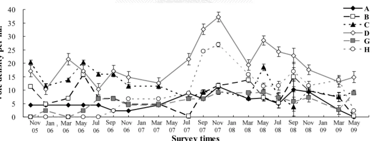
population dynamics of Taiwan voles at the six sampling plots over three and half years

were shown in Fig. 3. Taiwan vole populations showed spatial and temporal

heterogeneity at the study site. Population densities not only differed among plots, they

fluctuated in 2~3 folds magnitude over time at some plots. Generally, there were more

females than males (paired t-test, p < 0.01, 17.25 ± 1.03 females and 13.28 ± 1.07 males

per hectare, Fig. 4).

0 5 10 15 20 25 30 35 40

0 60 120 180 240 300 360 420 480 540 600 660 720 780 840 900 960 1020 1080 1140 1200 1260 1320 1380

Survey times

Vole density per ha.

A B C D G H

Fig. 3.Vole density (number per hectare) at each sampling plot from Oct.2005 to May 2009, estimated with the Pradel model in Program MARK. Error bars represent ±1se.

Fig. 4. The number of male and female voles from Oct.2005 to May 2009, estimated with the Pradel model in Program MARK. The error bars represent ± 1se.

0 10 20 30 40 50 60

Oct/05 Dec/05

Mar/06 May/06

Jul/06 Sep/06

Nov/06 Jan/07

Mar/07 May/07

Jul/07 Sep/07

Nov/07 Jan/08

Mar/08 May/08

Jul/08 Sep/08

Nov/08 Jan/09

Mar/09 May/09 Survey time

The number of individual

Male Female Total

Daily defecation rates of voles

Daily defecation rates ranged from 5.16 to 9.41 g per day per vole. There was no

difference between male and female voles (Mann-Whitney U test, U = 150, p = 0.75)

within each month, samples were pooled between sexes. Voles defecated more feces in

cold (Jan.-10 and Mar.-08) than warm (Apr.-09 and Jul.-07) months (Kruskal-Wallis test,

H = 18.07, d.f. = 3, p < 0.01; Fig 5). The March-08 sample was lost due to preservation

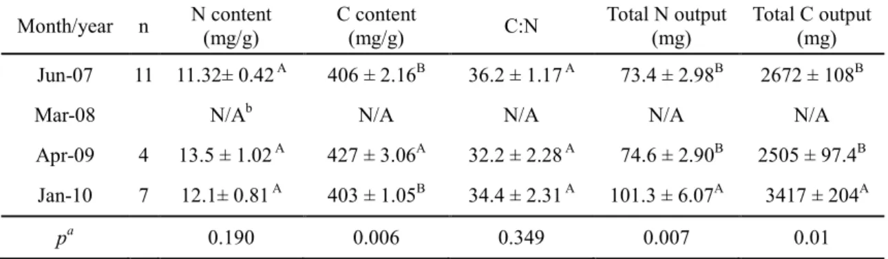
problem before chemical analyses could be performed. Carbon content per gram feces

in Apr.-09 was higher than Jul.-07 and Jan.-10, although nitrogen content per gram

feces was not different between months (Table 3). The daily total nitrogen output

(Kruskal-Wallis test, H = 9.79, d.f. = 2, p = 0.007; Table 3) and total carbon output (H =

9.30, d.f. = 2, p = 0.01) per vole were both higher in Jan.-10 than other months caused

by differential fecal output.

Fig. 5. Daily defecation rates (mean±1se) of voles in different month/year. Different alphabets indicate significant differences based on Kruskal-Wallis test. n = 12, 10, 10, 5, left to right, respectively.

0 2 4 6 8 10

Jul-07 Mar-08 Apr-09 Jan-10

Month

F ea c es w ei g h t (g )

b b

Table 3. The N and C content in vole feces (mg/g), and total N and C output of vole feces per vole produced after 24 hrs in the laboratory. All values give mean±1se.

Month/year n N content (mg/g)

C content

(mg/g) C:N Total N output

(mg)

Total C output (mg) Jun-07 11 11.32± 0.42 ^A 406 ± 2.16^B 36.2 ± 1.17 ^A 73.4 ± 2.98^B 2672 ± 108^B

Mar-08 N/A^b N/A N/A N/A N/A

Apr-09 4 13.5 ± 1.02 ^A 427 ± 3.06^A 32.2 ± 2.28 ^A 74.6 ± 2.90^B 2505 ± 97.4^B Jan-10 7 12.1± 0.81 ^A 403 ± 1.05^B 34.4 ± 2.31 ^A 101.3 ± 6.07^A 3417 ± 204^A

p^a 0.190 0.006 0.349 0.007 0.01

a. Different alphabets in a column indicate significant differences based on Kruskal-Wallis test.

b. The Mar-08 sample was lost due to preservation problem.

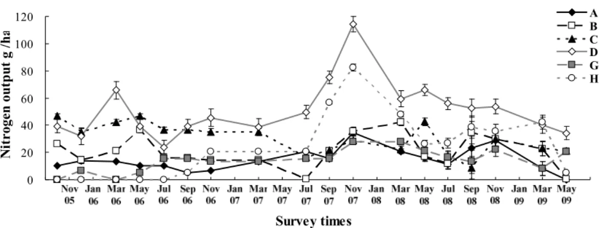
Nitrogen output of vole populations

Yeh (2010) observed that Yushan cane at the study site showed little growth and

had low quality for voles during November to March. I used the average of feces data

(Table 3) from January-10 and March-08 to represent non-growing season; and the

average of April-09 and July-07 to represent growing season. I multiplied daily

defecation rate by the nitrogen content of feces to obtain daily nitrogen production per

individual vole for each season. The values were multiplied by monthly vole density

estimates, then by 30 (days) to give monthly nitrogen output by vole feces per hectare

(Fig. 6). The values were influenced largely by vole population sizes, ranged from 0 to

114 g ha^-1 month^-1. The annual nitrogen output per Taiwan vole came to be 32.45 g

year^-1.

0 20 40 60 80 100 120

0 60 120 180 240 300 360 420 480 540 600 660 720 780 840 900 960 1020 1080 1140 1200 1260 1320 1380

Survey times

Nitrogen output g /ha

A B C D G H

Fig. 6. Nitrogen output of voles in different months. Nitrogen output was calculated by vole density of survey month multiplied by vole daily nitrogen output. Error bars represent ±1se.

0 5 10 15 20 25 30 35 40 45 50

Jul-07 Sep-07 Nov-07 Mar-08 May-08 Jul-08

Survey times

N u m b e r o f la tr in e

Fig. 7. Number (mean±1se) of vole latrines per 100 m² in each plot. The values gave averages of the two quardrats in the same plot. Latrine survey quadrats at plot G and H were not set up until September 2007.

0 10 20 30 40 50 60 70 80 90 100

10~20 20~40 40~60 60~80 80~100 100~120 120~200 ≧≧200≧≧ The number of fecal pellets in latrine

Counts

Fig. 8. Frequency distribution of the number of fecal pellets in latrines (n = 263). The number of fecal pellets in latrines ranged from 10 to approximately 700.

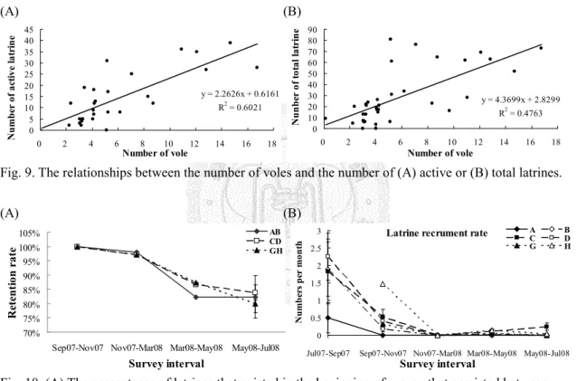
Vole latrines survey

I recorded a total of 263 vole latrines during July 2007 to July 2008

.

dynamics of latrine numbers showed substantial spatial heterogeneity (Fig. 7). The fecal

pellets in latrines ranged from 10 to approximately 700, and mostly between 20~40 (Fig.

8). I defined “active latrines” as newly recorded latrines and those that new pellets had

been added to old latrines since last survey (Table 4). The numbers of active latrines (r =

0.78, Fig. 9A) and total latrines (r = 0.69, Fig. 9B) were both highly positively

correlated with the number of voles. The survival rates of latrines, i.e., the percentages

of latrines persisted between surveys were generally over 80% (Fig. 10A). After

excluding pre-existing latrines, and those persisted beyond the final survey, average

persistent time of latrine was 6.82 ± 0.29 months (n = 89). It’s certainly an

underestimation, for example, thirty-one latrines persisted for more than 1 year. The

inclusion of those latrines would bring the average persistence time of latrine to 8.36 ±

0.18 months (n = 120). The recruitment of new latrine was the highest during July to

September; and the lowest during November to March (Fig. 10B & Table 5). The reuse

rates of latrines ranged from 11.1~57.1% (Table 5). The dispersion pattern of latrines in

each quadrat was all random (based on spatial analyses, results not shown), but the

numbers of latrine between quadrats were highly variable.

Table 4. The number of voles and latrines, both active and total, during bimonthly surveys. Active latrines were newly recorded latrines and those that new pellets had been added to old latrines. Total latrines were all latrines recorded, including non-active ones.

Plot A B C D G H

Vole Active Total Vole Active Total Vole Active Total Vole Active Total Vole Active Total Vole Active Total

+^a new + new + new + new + new + new

Jul/07 4 - - 4 0 - - 9 3 - - 6 10 - - 16 3 - - - 4 - - - Sep/07 3 2 3 7 4 1 17 26 4 1 11 17 15 3 36 52 3 -^b - 13 11 - - 28 Nov/07 5 0 0 6 5 3 5 31 4 4 9 21 17 17 11 73 4 5 4 17 12 4 31 69 Mar/08 3 3 0 6 6 5 3 34 3 4 0 22 9 11 1 65 4 3 2 19 7 16 9 76 May/08 3 1 1 6 3 5 0 21 8 12 3 23 13 27 0 63 4 7 0 15 5 20 11 81 Jul/08 2 2 0 5 2 12 0 20 3 13 6 24 11 36 0 62 3 5 0 13 5 14 3 61 a. “+” indicates the number of active latrines due to new fecal pellets.

b. Latrine survey quadrats at plot G and H were not set up until Sep-07.

(A) (B)

y = 2.2626x + 0.6161 R² = 0.6021

0 5 10 15 20 25 30 35 40 45

0 2 4 6 8 10 12 14 16 18

Number of vole

Number of active latrine

y = 4.3699x + 2.8299 R² = 0.4763 0

10 20 30 40 50 60 70 80 90

0 2 4 6 8 10 12 14 16 18

Number of vole

Nunber of total latrine

Fig. 9. The relationships between the number of voles and the number of (A) active or (B) total latrines.

(A) (B)

70%

75%

80%

85%

90%

95%

100%

105%

Sep07-Nov07 Nov07-Mar08 Mar08-May08 May08-Jul08 Survey interval

Retention rate

AB CD GH

Latrine recrument rate

0 0.5 1 1.5 2 2.5 3

Jul07-Sep07 Sep07-Nov07 Nov07-Mar08 Mar08-May08 May08-Jul08

Survey interval

Numbers per month

A B

C D

G H

Fig. 10. (A) The percentages of latrines that existed in the beginning of survey that persisted between surveys. (B) Latrine recruitment rates, (the number of new latrines occurred between surveys, in each plot, estimated using Program Mark). Latrine survey quadrats at plot G and H were not set up until September 2007. Error bars represent ±1se.

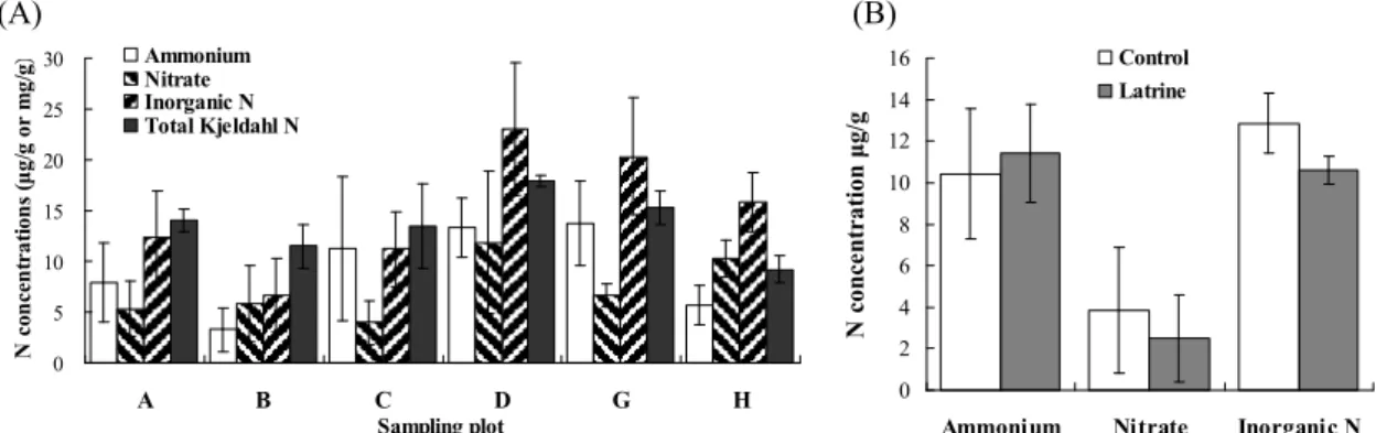
Field Incubation on Natural Soil

The initial N contents of soil (collected in July 2007) were quite variable spatially

(Fig. 11A), ranged from undetectable (concentration under 0.5 µg/g was not detectable

by the method used) to 41 µg/g. After two months, the N contents of soil underneath

artificial latrines and control soil (collected in September 2007) were not significantly