以核苷酸k聚體頻度分類序列

(1)

國立臺灣大學電機資訊學院生醫電子與資訊學研究所碩士論文

Graduate Institute of Biomedical Electronics and Bioinformatics College of Electrical Engineering and Computer Science

National Taiwan University Master Thesis

以核苷酸 k 聚體頻度分類序列

Sequence Classification Based on kmer Frequencies

陳泓宇 HungYu Chen

指導教授：趙坤茂博士 Advisor: KunMao Chao, Ph.D.

中華民國 108 年 7 月

July, 2019

(2)

(3)

誌謝

首先要感謝我的指導教授趙坤茂老師，從我大學至今多年來給予我非常多指導與幫助。在我大學階段，老師擔任我的導師時就常常關心我，有時也在我的求學生涯上提供相當有用的指引，偶爾在導生宴時聽到老師與學長姐們討論演算法更是啟發了我對演算法的興趣。研究所時有幸進入趙老師的實驗室，感謝老師給予我們非常大的自由，讓我能隨心所欲的探索有興趣的領域，而對於我想發展的各個課題也總是會提出精闢的建議與我討論，提供我很多幫助。

感謝實驗室同伴們營造了一個自在而適於研究的空間，讓我在研究的過程中能夠非常順利，有疑惑時能一起討論，要趕進度時能一起努力。感謝實驗室學長們在我每學期的報告中給予我建議及鼓勵，讓我的研究主軸能漸趨完整。也感謝射箭社中時常關心我研究進度的學弟妹、學長姐，以及互相督促的研究生夥伴們，讓我在這兩年中總是有個地方可以放鬆心情。

最後感謝我的家人，在這二十多年中給予我支持與鼓勵，讓我可以一直無後顧之憂的求學至今。

(4)

摘要

序列分類在計算生物學的許多研究中是一個在研究初期就需要解決之問題，有許多方法被研發出來計算此問題，但隨著高通量定序技術的發展，需要計算的資料量也大幅增加，導致許多現有方法已無法在 能取得的計算資源及可接受的時間內完成計算。以核苷酸 k 聚體為基 礎的演算法就是其中一種，目前已有不少方法可以快速且準確的完成分類，但卻需要大量的計算空間，因此無法在一般個人電腦中完成計算。

在本篇論文中，我們提出一個以核苷酸 k 聚體為基礎的演算法，在 時間上與現有方法相當，在空間上則避免現有方法中儲存上的冗餘性而做出改善。為進一步降低所需記憶體空間，我們提出一個分割架構，

此架構除了可以減少所需空間，也適合平行化以縮短計算所需時間。

關鍵字：序列分類、環境基因體學、基因體學、k 聚體、免序列比對、

序列特徵、演算法

(5)

Abstract

Sequence classification is a preliminary step in many researches of computational biology. There are a variety of methods proposed to compute this problem. However, with the development of highthroughput sequencing technologies, the datasets of sequencing data are getting much larger. As a result, many existing methods cannot accomplish this task with limited computational resource and acceptable time. The kmer based algorithms are some of these methods. Most of them could finish the classification fast and accurately, but they need large computational space, which is not available in common personal computers.

In this thesis, we propose a kmer based algorithm. The time complexity of our algorithm is comparable to those of the existing methods, while we make an improvement in space usage by avoiding the redundancy of storing the kmers. To further reduce the memory usage, we propose a partitioning strategy. In addition to the reduction in memory usage, the algorithm under this partitioning structure can be highly parallelized to improve performance.

Keywords: sequence classification, metagenomics, genomics, kmer, alignmentfree, sequence signature, algorithm

(6)

List of Figures

1.1 Sequence classification problem . . . 4

2.1 Human readable kmer spectrum file . . . . 10

2.2 Workflow of Simka . . . 12

2.3 Workflow of CLARK . . . 13

3.1 From a kmer to an element in the hash table . . . . 15

3.2 The construction of index hash tables with partitioning strategy . . . 21

3.3 The classification of an object dataset with partitioning strategy . . . 21

3.4 Index construction phase with multithreading . . . 23

3.5 Classification phase with multithreading . . . 23

(9)

List of Tables

2.1 Sizes of datasets and KMC3 output files . . . 10 3.1 Space complexity of both algorithms . . . 19 3.2 Time complexity of both algorithms . . . 19

(10)

List of Algorithms

1 BuildIndex . . . 16 2 Classify . . . 17 3 AlgorithmWithPartitioning . . . 22

(11)

Chapter 1 Introduction

A substring of length k in a given string, usually a sequencing read, is called a kmer in bioinformatics. For example, given a sequencing read ACGGTTC, all 3mers in this read are ACG, CGG, GGT, GTT, and TTC. With the development of highthroughput sequencing technologies, the studies of kmers are getting more and more important because many computational methods use kmers to analyze the sequencing reads and datasets. In other words, kmer is a fundamental unit for many methods [2, 25, 28, 29, 32, 62].

The number of the occurrences of each kmer in a given dataset is called kmer frequency or kmer spectrum, and the problem of computing kmer frequencies is called kmer counting. The kmers with high frequencies can be regarded as features of a dataset. In contrast, the kmers with low frequencies, such as kmers occurring only one time, which are called singleton kmers, are often generated by sequencing errors.

There are many methods and applications making use of kmer counting. For instance, genome assembly [4, 19, 41], estimation of genome size [57], read correction [23], repeat detection [8, 20, 26, 27, 34], sequence alignment [14] and comparison of genomes [9, 42, 64].

kmer counting is conceptually simple, but it is difficult to be both fast and memory

efficient. In particular, the sizes and the amounts of datasets nowadays are increasing rapidly. Some traditional kmer counting tools cannot complete the task of large datasets or large k in reasonable time and space. A naïve implementation of kmer counting is to

(12)

use a simple hash table, where keys are the kmers and values are the counts. However, when there are many distinct kmers, the hash table should be very large, which is often larger than given memory space, to avoid collisions. As a result, some studies make efforts to implement more spaceefficient data structures for kmer counting. There are also some studies trying to solve this problem by using disk space instead, which is a tradeoff between performance and space because disk I/O operations are much slower.

There are many latest researches [5, 18] about kmer counting.

kmers are widely used in metagenomics in recent years. For example, signa

ture kmers representing members of a certain protein family can be used to annotate metagenomes [15] and kmer frequencies can be used in binning metagenomic contigs [1].

An important application is the classification of sequences. In some researches, the sequences to be classified belong to the same metagenome, and the researchers want to know which metagenome it is. In some other researches, the researchers want to determine the identities of the species in the sequenced sample. A solution common to these two problems is to compare the given sequences with sequences of known origins. kmer frequencies can be very helpful in both cases. With analyzing and comparing the k

mer frequencies of the given sequences of the same metagenome/species to the kmer frequencies of the sequences of other determined metagenomes/species, we can get the dissimilarities and then infer the relationships between different datasets [6, 13, 45, 50].

Considering the properties of kmers and the fact that the computation of kmer frequencies is getting faster and uses much lower memory space than before, the sequence comparison based on kmer frequencies is promising. Some of the comparison methods mentioned above can use the output of the kmer counting tools as input, while some methods develop their own methods to count kmers. CLARK [45] is a fast classification method based on kmer frequencies which takes files containing kmer frequencies as input. Nevertheless, the memory usage of CLARK is too large for common personal computers. There is a variant of CLARK trying to solve this problem, but the accuracy gets lower. In this thesis, we propose the algorithms which not only overcome this issue but also improve the performance.

(13)

1.1 Motivation

The classification of datasets is an essential task in the preliminary stage of many researches. An intuitive approach is to measure the dissimilarities between datasets.

Sequence alignment is a traditional solution in taxonomy. Through analysing the results of the alignment, the evolutionary relationships between object datasets and reference datasets could be inferred. However, object datasets usually consist of sequencing reads, which are not suitable for alignment, and the assembly of reads from unknown origins is a difficult task. Therefore, alignmentfree methods are proposed. One category of these alignmentfree methods is based on kmers. Some properties of kmers, which are described in Section 2.2, make kmers appropriate for comparing datasets. Some k

mer based methods compute the pairwise distances between kmer spectra of datasets to measure the dissimilarities. Nonetheless, pairwise comparisons are timeconsuming.

An approach to avoid pairwise comparisons between datasets is to find the signature kmers of each dataset and classify the datasets according to these signature kmers. The criteria of finding the signature kmers is another critical issue. The kmers with highest frequencies may be candidates, but kmers occurring many times in one dataset could also occur many times in other datasets just because they are common in nucleotide sequences.

CLARK provides an intuitive and efficient approach to solve this problem. It finds the k

mers specific to each target dataset and classifies the object datasets accordingly. The disadvantage of CLARK is the large memory usage. As a result, we try to improve this method by reducing memory usage.

1.2 Problem Description

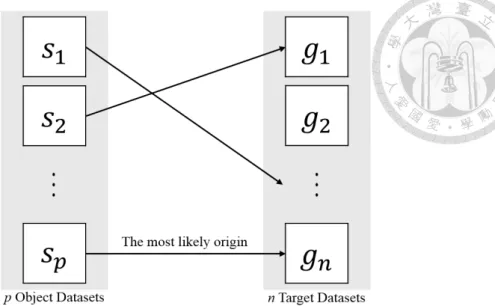
Given p object datasets to be classified and n target datasets of known origins, determine which target is the most likely origin of each object (Figure 1.1).

The datasets could be metagenomic or genomic sequences as long as all the sequences in the object and target datasets are grouped into datasets at the same level. It is also feasible to construct the datasets with the sequences grouped at species or genus level.

(14)

Figure 1.1: Sequence classification problem

In traditional methods, the definition of “the most likely origin” is the target with the smallest taxonomic dissimilarity. However, these methods usually need complete reference databases to compute the dissimilarities and they are computationally costly.

Consequently, many researchers attempt to find methods based on other data instead of the contents of the sequences. Some proposed methods make use of kmer frequencies.

There are some existing kmer based methods which could solve this problem fast. In this thesis, we focus on how to solve this problem fast and accurately on the basis of kmer frequencies with limited memory space.

1.3 Main Results

There is a fast and accurate method, CLARK, resolving this problem based on kmer frequencies. However, it uses large RAM space during the computation. In this thesis, we try to reduce the memory usage such that this task could be computed with common personal computers. We propose algorithms which avoid the redundancy of storing kmers in CLARK. The time complexities of these algorithms are the same as CLARK’s, while they should be faster than CLARK in practice. We also propose a partitioning strategy to further reduce the memory usage.

(15)

1.4 Organization of the Thesis

• Chapter 2 Related Work

In this chapter, we summarize some related work about kmer counting tools and kmer based comparative metagenomics methods. The algorithms of some kmer counting tools provide good ideas to improve classification methods. In addition, we conclude some researches indicating that kmers have some good properties such that they are suitable for comparing datasets.

• Chapter 3 Methods

In this chapter, we propose algorithms which overcome the issue of large memory usage. We describe the algorithms, analyze them and compare them with the existing kmer based classification method, CLARK. In addition, we propose a partitioning strategy to further reduce the memory usage of the purposed algorithms.

The algorithms with this strategy can be highly parallelized.

• Chapter 4 Conclusion

In this chapter, we conclude the proposed algorithms and the partitioning strategy.

Besides, we describe the direction of future work.

(16)

Chapter 2 Related Work

2.1 kmer Counting Tools

Although there are many studies based on kmer counting, early ones only consider it as a preliminary step and describe it sketchily. Tallymer [26] is the first tool designed specifically for kmer counting. Rather than hash table, this tool is based on suffix array.

Meryl is a kmer counting tool from the Celera assembler [41] package, which uses a sortingbased approach. However, these tools are not efficient enough to deal with large datasets.

Jellyfish [39] uses a multithreaded, lockfree hash table. Users have to prespecify the memory size for the hash table to use. Once the hash table is full, the intermediary kmer counts are saved to disk and merged to the final results later. Its current versions are still used commonly in recent studies.

BFCounter [40] points out that more than half of the observed kmers even in preprocessed datasets are singletons, which can be weeded out as wrong data caused by sequencing error and thus should not be inserted into the data structure for counting.

BFCounter uses a twopass method. In the first pass, it uses a Bloom filter [7] to filter out the kmers which occur only one time. The Bloom filter is an approximate membership query (AMQ) data structure. An AMQ data structure maintains a compact and probabilistic representation of a set or multiset, so it could generate false positives

(17)

into a hash table. Since the result of a query to the Bloom filter is probably a false positive, there may be some kmers occurring only once inserted into the hash table. In the second pass, it reiterates over all the reads and counts the kmers which are inserted in the hash table in the first pass using a hash table to get the exact frequencies. BFCounter uses less memory but much more time than Jellyfish. The difference in speed is mainly due to the twopass method. It is feasible for BFCounter to do the counting in the first pass and omit the second pass to obtain approximate kmer frequencies.

Jellyfish and BFCounter mainly rely on memory, and usually need dozens of gigabytes of memory, which are not available in most personal computers. Relatively, it is much easier to get sufficient capacity from disks. Consequently, some studies try to develop diskbased kmer counting tools, such as DSK [51] and KMC [11, 12, 24]. DSK relies on hash tables. Different from Jellyfish, it processes the kmers in several iterations. In each iteration, only a partition of kmers classified according to their hash values are saved to their corresponding lists in the disk and then the lists are read from the disk to insert into a hash table for counting. Users can set the target memory usage size and the target disk space size. The numbers of iterations and lists are calculated accordingly, so it is guaranteed that the size of hash tables would not exceed the target memory usage size.

KMC [11] is similar to DSK in concept. The major difference is that KMC has developed a scheme of parallel algorithm. The whole process can be divided into two phases. In distribution phase, the kmers are partitioned into several bins on the basis of their prefixes, sorted and compacted. The bins are then stored into disk as files. In sorting phase, the files are read from the disk. Kmers are uncompacted, sorted and counted.

Turtle [54] uses a method similar to BFCounter. It uses a patternblocked Bloom filter [49], which reduces the number of cache misses by restricting the locations to store a kmer in the filter, to filter out singleton kmers. The kmers occurring more than once are stored in an array. By repeatedly sorting and compaction, users can get the array of these kmers with their counts.

KAnalyze [3] implements a modified merge sort algorithm to count kmers, and the algorithm could be divided into two components: split component and merge component.

(18)

The split component reads a set of kmers into an array and sorts the array with a dual

pivot quicksort algorithm. Then, it counts the kmers by traversing the array, writes the kmers with their counts to a file in disk and fills the array with the next set of kmers. The merge component reads the files and accumulates the counts.

khmer [63] uses an AMQ data structure, countmin sketch [10], to count the kmers.

Different from other methods, khmer does not store kmers in the data structure. To increment the count of a kmer, it uses a hash function to get the hash value and determines the locations to be updated in the hash tables of the countmin sketch accordingly. To retrieve the count of a kmer, the hash value is computed and the minimum count among the counts in all hash tables is returned. However, there are miscounts in the results of khmer because the countmin sketch could generate false positives. khmer provides a way to systematically trade larger memory usage for lower false positive rate.

There is high redundancy in above methods. Consecutive kmers share k–1 symbols, but they are processed and stored as kmers not relevant at all. MSPKmerCounter [30]

introduces minimizers [52, 53] to the kmer counting problem to reduce the redundancy.

KMC 2 [12] refines the minimizers to signatures, which fit the parallel scheme of KMC better. In distribution phase, it partitions super kmers consisting of kmers sharing the same signatures into bins according to their signatures. In sorting phase, it breaks down super kmers and counts them in an approach similar to the method in KMC. KMC 3 [24]

follows the same scheme as KMC 2 and makes some improvements in details.

KCMBT [37] counts kmers on the basis of multiple burst tries [21, 56]. It inserts k

mers into burst tries and traverses the tries to get the final kmer frequencies after inserting all the kmers. KCMBT constructs 4^aburst tries, where a is the prefix length for indexing the tries, to reduce the space for storing kmers.

Gerbil [16] uses a diskbased and parallel approach similar to KMC 2. It is divided into two phases as well: distribution phase and counting phase. In distribution phase, it uses minimizers to split the input data into several smaller temporary files which are stored in the disk. They experimentally evaluated various ordering strategies of minimizers, and they found the strategy, signatures, used by KMC 2 is a good choice for most datasets. In

(19)

counting phase, the temporary files are reread from the disk. After splitting super kmers into kmers. Gerbil uses the hash table approach to count the kmers and solves collisions via quadratic hashing. In addition, Gerbil puts emphasis on algorithm engineering. It points out several details implemented to gain high performance and utilizes GPUs to speed up the counting phase. Gerbil can support the counting of kmers for large k of large datasets, which cannot be finished efficiently by KMC 2 and not supported by DSK.

Squeakr [47] uses counting quotient filters [46] to count the kmers. The counting quotient filter (CQF) is a novel AMQ data structure, but the collisions can be avoided by adjusting the size of hash function and the size of data to be stored. Squeakr extracts the kmers from input data and inserts them into a local CQF in each thread. The data in the local CQFs are then inserted into a global CQF to get the final approximate results. It is possible for Squeakr to get exact results by adjusting the CQFs as mentioned above, and it is called Squeakrexact.

There is a benchmark study [38] of the kmer counting tools. They find that KMC3, DSK and Gerbil are the most flexible and efficient. (Squeakr is not assessed in this study.) It seems that the sizes of the output files of kmer counting tools would be very large when k is large because of the redundancy of kmers. Conceptually, if all possible kmers occur, there would be 4^k kmers stored in the file with their counts. In practice, there would not be so many kmers in the output files because (1) some kmers hardly occur due to the molecular structure of nucleic acids, (2) kmers are counted in canonical form (the lexicographically smaller one among the kmer and its reverse complement) because when a kmer occurs, there must be its reverse complement occurring on the other strand, and (3) many kmer counting tools filter out singleton kmers in default, and these singleton kmers usually account for a large proportion of the kmers. In addition, in most kmer counting tools and applications based on kmers, the kmers are stored in binary form. A is encoded as 00, C as 01, G as 10 and T (U) as 11 such that each four bases of a kmer can be stored in one byte. Take KMC3 for example, it filters out kmers occurring less than 2 times in default and stores the kmers in binary form. To compact the sizes of output files with reducing the redundancy of kmers, it divides the output into prefix file (.kmc_pre)

(20)

and suffix file (.kmc_suf). We compute the kmer spectra of some datasets with KMC3 to show that kmer spectrum is a succinct representation of sequence datasets (Table 2.1).

However, it is a lossy representation. There is no information of kmer position kept in the spectrum.

Organism Genome length Dataset FASTQ

files size

Gzipped files size

Output files size with/without filtering

E. coli 5 SRR5002442 3.71 1.24 0.14/1.35

C. elegans 102 DRR008444 19.62 5.95 0.78/1.71

F. vesca 214 SRA020125 9.52 3.38 2.22/5.43

Table 2.1: Sizes of datasets and KMC3 output files. k = 31. FASTQ and gzipped files are the datasets, and most kmer counting tools could take both of these formats as inputs.

Genome lengths are in Mbases according to http://www.ncbi.nlm.nih.gov/genome/. File sizes are in Gbytes (1 Gbyte = 10⁹ bytes). For output files with filtering, we set KMC3 to filter out kmers occurring less than 2 times. The datasets were downloaded from https://www.ebi.ac.uk/ena.

KMC3 provides a tool to convert output files to human readable kmer spectrum files.

The kmer spectrum contains the kmers and their frequencies (Figure 2.1).

Figure 2.1: Human readable kmer spectrum file

2.2 kmer Based Metagenomic Comparison and Classifi

cation Methods

A traditional method to determine the origin of a set of sequences is sequence alignment with reference sequences. But this method is not feasible when the reference databases are not complete. The lack of reference databases especially exists in metagenomics [22]. As a result, some researchers proposed de novo methods. A method [31] measures dissimi

larities between datasets by marker genes and cluster them, but they are computationally

(21)

expensive and leave lots of the reads unused. Therefore, another method [61] compare read contents directly with BLAST [2]. However, these methods cannot scale up to large datasets.

kmer based methods are introduced into this issue in recent years. In [6], it states that

“kmers are a natural unit for comparing communities:

• sufficiently long kmers are usually specific of a genome [17],

• kmer frequency is linearly related to genome’s abundance [60],

• kmer aggregates organisms with very similar kmer composition without need for a classification of those organisms [58].”

There is also a research [13] comparing kmer based distances and taxonomic distances based on assignation against reference databases. They find that kmer based distances are well correlated to taxonomic distances. Additionally, the kmer based distances overcome the incompleteness issue of reference databases.

Compareads [36], Commet [35] and another method [55] compute the similarities between datasets based on the number of shared kmers. MetaFast [59] and Mash [43]

compute pairwise similarity matrices using feature vectors of kmer composition.

Simka [6] computes varieties of distances between multiple datasets based on kmer frequencies. To compute distances between multiple datasets simultaneously, the kmer frequencies of all the datasets are needed. If we attempt to compute distances after finishing the counting of the frequencies of all the kmers in datasets, we have to record a matrix of size W× N, where W is the number of distinct canonical kmers and N is the number of datasets. When W and N are large, this matrix would require a large amount of space. To avoid this demand for large space, Simka develops an efficient multiset k

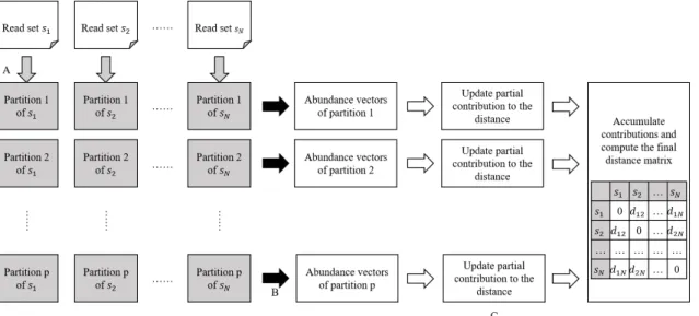
mer counting algorithm (MKC) and applies some ecological distances which are additive over kmers. To compute these distances, Simka only has to compute the distances using a part of the kmers in each step, and aggregates the results of all the parts to get final distances (Figure 2.2). After extracting and storing the canonical representation of each kmer, MKC separates the kmers into a fixed amount of partitions. Each partition is

(22)

then sorted, counted and stored as files in disk independently. Thus the files associated to the same partition contain a specific subset of kmers common to all datasets. With this partitioning strategy, Simka only takes a part of the counts at a time to compute the distances. Moreover, this approach is suitable for parallelization.

Figure 2.2: Workflow of Simka. (A) The gray arrows represent the sorting count processes of MKC. Each process outputs p partitions of sorted kmer counts. (B) The black arrows represent the merging count processes of MKC. Each process merges the counts in N partitions of a common subset of kmers and outputs abundance vectors of these kmers. (C) Simka uses the abundance vectors to update independent contributions to the distance. In final step, it accumulates contributions to compute the final distance matrix.

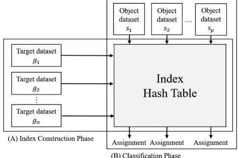
CLARK [45] classifies the datasets using discriminative kmers. It builds a large index hash table containing the kmer spectra of all target datasets and removes the kmers occurring in more than one dataset. The remaining kmers are discriminative (target

specific) kmers which could be regarded as representatives of corresponding datasets because each of these kmers exist in the dataset uniquely. As a result, the targetspecific kmer sets of all the target datasets are obtained (Figure 2.3 (A) Index Construction Phase).

To classify an object dataset, for each kmer in the dataset CLARK queries the index hash table to check if this kmer matches a targetspecific kmer of a dataset. If so, it is called a

“hit.” After querying all the kmers, the object is assigned to the target dataset having the highest number of hits (Figure 2.3 (B) Classification Phase). CLARK offers two modes

(23)

of the first assignment and the number of hits against all the targets. The default mode stops querying for an object as soon as there is one target collecting half of possible hits and only outputs assignments. There is a variant, CLARKE, significantly accelerating the computation of classification while maintaining high precision and sensitivity. It only queries nonoverlapping kmers and assigns the object to the first target that obtains a hit.

Figure 2.3: Workflow of CLARK

Besides high accuracy and speed, the major advantage of CLARK is that it provides an intuitive approach to find the signature kmer sets. However, it uses large memory space while constructing the index hash table. For example, the RAM peak usage of the database construction of 2,752 bacterial genomes is 164.1 GB, which is not available in some workstations and most personal computers. There is another variant, CLARKl, designed for machines with limited amounts of RAM. CLARKl constructs a smaller hash table and smaller discriminative kmer sets. It uses smaller k and samples a fraction of k

mers of each target datasets to build the index. In the experiment mentioned above, the RAM peak usage of CLARKl is only 3.8 GB. Nevertheless, the sensitivity and precision of CLARKl is much lower in some cases. A method called CLARKS [44] was proposed later to improve the sensitivity of CLARK on the basis of the idea of spaced seed [33].

Compared to CLARK, its memory usage for classification is even larger and its running time is much longer.

(24)

Chapter 3 Methods

CLARK provides an intuitive and efficient approach to find out the discriminative kmer sets of target datasets and classify object datasets. However, there are some redundant computations in the algorithm of CLARK which may lead to large memory usage. We have devised an algorithm which removes the redundancy of CLARK.

In the algorithm of CLARK, the part using the most memory space is the index hash table. There are 4^k possible kmers in the kmer spectrum of a dataset, so the kmer spectrum is a vector of dimension 4^k. To avoid too many collisions, CLARK builds large hash table and uses separate chaining. It simply inserts the IDs for all the targets containing a certain kmer to the list of this kmer. When the kmer is common in many datasets, the list would be long and take up lots of space. In fact, the kmer existing in more than one dataset would be removed afterwards. As a result, it is a waste of computation resource to store the same kmer of all the datasets containing this kmer in the hash table. In addition, there are some values stored in the hash table not necessary in the algorithm, so we also modify the data structure of the kmer storing in the hash table.

3.1 Algorithm

The algorithms in this thesis focus on the construction of the index hash table and the classification of object datasets. The computation of kmer frequencies can be finished fast and memoryefficiently using the kmer counting tools mentioned in related work.

(25)

The inputs of the whole algorithm are (1) the kmer spectra of target datasets, (2) the kmer spectra of object datasets, and optionally (3) a minimum number of occurrences if user wants to remove kmers occurring less than a certain amount of times.

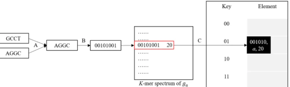
In this algorithm, the data structure of the kmers stored in the index hash table contains (1) the kmer, (2) the ID of the target dataset, and (3) the count of the kmer in the dataset. In fact, the count could be replaced with a Boolean variable because the frequency would not be used afterwards. We describe the algorithm with the count for convenience. Assuming that the input kmer spectra are counted in canonical form (Figure 3.1 arrow A) and stored in binary form (Figure 3.1 arrow B), we use a hash table the same as that designed in CLARK, a hash table of size L with separate chaining. The hash function h is defined as h(l) = l mod L, where l is the value of the kmer. With this hash function, we store the value l/L in the bucket h(l) of the hash table (Figure 3.1 arrow C). It is trivial to get the original kmer from the value stored in the hash table. The value of L is set to a power of 2 such that the modulo operation and division operation could be done easily with dividing the binary form of a kmer into two parts and taking the second part as hash value and the first part as the value to store in the element .

Figure 3.1: From a kmer to an element in the hash table

In Algorithm 1, we describe the method of building the index hash table. The algorithm attempts to store all the kmers into the hash table. If user has specified a minimum number of occurrences, the kmers with frequencies lower than this number should not be stored in the index. This examination is useful especially for the datasets with low sequencing quality because most of the kmers with low frequencies arise from sequencing errors.

When storing kmers in each dataset into the hash table, the algorithm would attempt to store identical kmers from different datasets into the same bucket of the hash table based

(26)

on the hash function. Rather than the exact frequency of each kmer, what is crucial in this algorithm is whether a kmer occurs in only one dataset. Based on this observation, when the algorithm tries to store a kmer into a bucket with the same kmer from a different dataset already stored in it, this new kmer should be ignored. On the other hand, the k

mer which has been stored in the bucket cannot be used as a targetspecific kmer either, but it would not be removed because it is kept as a token to record that this kmer exists in at least two datasets. The algorithm sets the count of the kmer to 0, representing that this kmer is merely kept as a token, so it would be removed afterwards and not included in the targetspecific set. For convenience of understanding the algorithm, we check whether the count of the stored kmer is equal to 0 in Algorithm 1. In practice, we could set the count to 0 without checking to save the time of checking the condition of the if statement.

After processing all the kmers from all the datasets, there is only one element stored in the index hash table for each distinct kmer. For each element, the value of count is either 0, representing this kmer should be removed, or a positive integer, representing the frequency of this kmer in corresponding dataset. After removing the kmers with counts equal to 0, the algorithm saves the index hash table in disk.

Algorithm 1 BuildIndex

Input: kmer spectra T (gc) of n target datasets (g_c)₁_≤c≤n

1: create an empty hash table H

2: for c = 1 to n do

3: for each kmer km with frequency cntcin T (g_c) do

4: if cnt_c≥ minoccur then

5: if there is (km, i, cnti)∈ H then

6: if cnti = 0 then

7: do nothing

8: else

9: cnt_i = 0

10: else

11: insert (km, c, cnt_c) in H

12: for each (km, i, cnti)∈ H do

13: if cnt_i = 0 then

14: remove this element

15: store the index hash table in disk

(27)

After constructing the index hash table, we can use it to classify the object datasets.

In Algorithm 2, we describe the method to classify object datasets. It is conceptually the same as the algorithm of the classification part of CLARK’s algorithm. We modify it such that the algorithm fits the structure that we propose later and keep the computation of the statistics which are computed in CLARK. Using the same hash function, the algorithm checks whether each kmer in the kmer spectra of object datasets exists in the target

specific kmer set of a target dataset easily. If so, it is a hit and the algorithm counts the hits by adding the frequency of this kmer in the object dataset to the counter of corresponding target dataset. After counting all the hits, we calculate the statistic γ. | T (sl)| is the total number of kmers in object dataset l. γ indicates the proportion of kmers which hit the targetspecific kmer sets of target datasets. If γ = 0, it means that none of the kmers in the object dataset hits target datasets and the algorithm cannot classify this object. Otherwise, the algorithm finds out the targets with the highest and secondhighest numbers of hits and computes the confidence score of the assignment to the highest target accordingly.

Algorithm 2 Classify

Input: index hash table H; n: the number of target datasets; kmer spectra T (sl) of p object datasets (s_l)₁_≤l≤p

1: for l = 1 to p do

2: declare n integer b1, b2, ..., bn= 0

3: for each kmer km with frequency cntlin T (s_l) do

4: if there is (km, i, cnt_i)∈ H then

5: bi = bi+ cntl

6: γ =∑n

t=1 bt

|T (sl)|

7: if γ = 0 then

8: output l, “not assigned”

9: else

10: m1 = arg max{b1, b2, ..., bn}

11: m₂ = arg max{{b1, b₂, ..., b_n} − {bm1}}

12: conf idence = _b ^b^m1

m1+b_m2

13: output l, b1, b2, ..., bn, γ, m1, m2, conf idence

(28)

3.2 Analysis of the Algorithms

In this section, we analyze and compare our algorithms with the algorithm of CLARK. To analyze the space complexity, we analyze the peak memory usage.

In index construction phase, the peak usages of both algorithms occur when the algorithms finish processing all the kmers of target datasets. CLARK simply inserts all the kmers of target datasets into the index hash table, so the number of elements inserted into the hash table is equal to the total number of the distinct kmers in the datasets.

Conceptually, there are 4^k total possible kmers in a dataset. In fact, for each dataset of genome length g, there are O(g) distinct kmers because there are s− k + 1 kmers in a sequence of length s. When the value of k is large, g is much smaller than 4^k. For example, when we set k to 31, 4³¹ is 4.6× 10¹⁸, while the length of the largest known genome is 1.5× 10¹¹ bp [48]. For all target datasets of total genome length G_T, there are O(G_T) distinct kmers. On the other hand, when k is small, there are O(n× 4^k) distinct kmers.

As a result, there are O(min(G_T, n× 4^k)) distinct kmers in general. Considering the size of the hash table L, the space complexity of CLARK is O(max(L, min(GT, n × 4^k))).

In our algorithm, for each distinct kmer, we store at most one element in the hash table.

However, the worst case is that the kmers of each target dataset are distinct in all the datasets, so we should store the same number of kmers in the hash table as CLARK. As a result, the space complexities of our algorithm and CLARK are the same. But there are many repetitive kmers in general, and our algorithm saves the space for storing these kmers. Suppose that a kmer occurs in r datasets on average, CLARK stores r times as many kmers as as we do.

In classification phase, after removing the elements of identical kmers from different datasets in CLARK, the peak usages of both algorithms are the same. The space complexities of both algorithms in this phase are equal to the space complexity of the completely built index hash table, which only contains targetspecific kmers. The worst case is the same as the case mentioned above, and all the kmers are targetspecific k

mers. Consequently, the space complexity of this phase is the same as the complexity of the index construction phase (Table 3.1).

(29)

Index Construction Classification Total

O(max(L, min(G_T, n× 4^k))) O(max(L, min(G_T, n× 4^k))) O(max(L, min(G_T, n× 4^k))) Table 3.1: Space complexity of both algorithms

The time complexities of our algorithm and CLARK’s algorithm are the same because the structure is basically the same. In index construction phase, the operations performing on each kmer could be done in constant time. There are O(min(G_T, n× 4^k)) kmers in total, so the time complexity of this phase is O(min(G_T, n× 4^k)). In classification phase, for each object dataset of genome size g, it takes O(min(g, 4^k)) time to count the hits of the dataset. The declaration of integers, the search of the targets with highest numbers of hits and the computation of γ take O(n) time. In general, O(min(g, 4^k)) is much larger than n. So for p object datasets of total genome length G_O, it takes O(min(G_O, p× 4^k)) time (Table 3.2).

Index Construction Classification Total

O(min(G_T, n× 4^k)) O(min(G_O, p× 4^k)) O(min(G_T, n× 4^k) + min(G_O, p× 4^k)) Table 3.2: Time complexity of both algorithms

Although the time complexities of both algorithms are the same, our algorithm should be faster than CLARK’s algorithm in practice. CLARK inserts all the kmers in the hash table and then removes most of them, and we prevent this waste by only storing the first occurring kmers.

Note that the peak memory usage of our algorithm is close to the peak memory usage in the classification phase of CLARK because the elements in the index hash table are the same. In the experiment of 2,752 bacterial genomes mentioned in the previous chapter, the RAM peak usage of classification phase of CLARK is 70.1 GB, which is still large for personal computers. In the next section, we provide a strategy to further reduce the memory usage.

(30)

3.3 Partitioning Strategy

Inspired by the idea of MKC in [6], we propose a structure based on a partitioning strategy to further reduce the peak memory usage of our algorithm. In the algorithm, it stores all the kmers of all the target datasets into a hash table, resulting in a hash table of large size.

However, when the algorithm searches for a hit of a kmer of an object dataset, at most one bucket containing corresponding kmer is needed. That is, we only need to obtain the bucket containing this element in the hash table. Conceptually, when we want to query a kmer, we can get the key value of the kmer using the hash function and load the bucket of this key value from disk. With this approach, the classification phase could be completed within small memory space. Nonetheless, it would give rise to excessive disk accesses, causing a large increase of running time.

To make a tradeoff between memory usage and performance, we partition all the k

mers into q parts according to their lexicographical order. The value of q is adjustable based on the specification of each machine. Some kmer counting tools print the kmers with their frequencies in lexicographical order in output files while some tools don’t. If not, we sort the kmers in the files as a preliminary task. It is easy to partition the sorted k

mers such that a partition contains a specific subset of kmers common to all datasets.

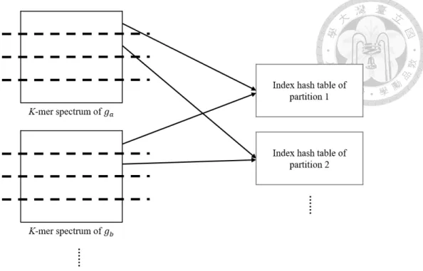
In index construction phase, we construct an index hash table independently for each partition. We take the same partition of each file to construct the same hash table of this partition (Figure 3.2). We use the same algorithm to construct the index hash tables of the partitions. In classification phase, we partition the kmers with the same rule. To classify an object dataset, we count the hits of each partition of kmers with the index of the partition (Figure 3.3).

This partitioning strategy can be applied to our algorithm with small modification (Algorithm 3). With this partitioning strategy, we only have to load a hash table of a partition in memory at a time during the construction and the classification of the partition. The space complexity of the original index hash table in our algorithm is O(max(L, min(G_T, n × 4^k))). With partitioning the kmers into q parts, this can be reduced to O(max(L,min(GT,n×4^k))

). Users could adjust the value of q to fit the RAM size

(31)

Figure 3.2: The construction of index hash tables with partitioning strategy

Figure 3.3: The classification of an object dataset with partitioning strategy of the machine. The number of kmers processed in total is the same as that in the original structure without partitioning, so the time complexity is still O(min(GT, n×4^k)+

min(G_O, p× 4^k)). However, the execution time in practice would increase as the number of partitions increases because of the relatively timeconsuming disk accesses of storing and loading the index hash tables.

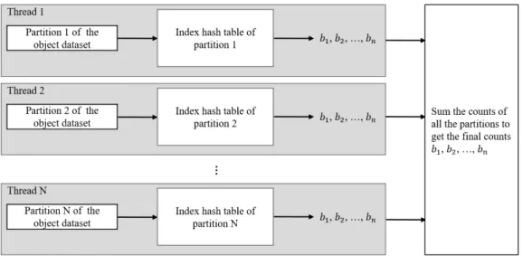
Another advantage of this partitioning strategy is that the algorithm with this strategy can be highly parallelized. For example, in index construction phase, each thread takes a partition of the kmers in all the target datasets to construct the index hash table of the partition simultaneously (Figure 3.4). In classification phase, each thread takes a

(32)

Algorithm 3 AlgorithmWithPartitioning

Input: q; kmer spectra T (gc) of n target datasets (gc)1≤c≤n; kmer spectra T (sl) of p object datasets (s_l)₁_≤l≤p

1: for each T (x_y) do

2: partition T (xy) into q parts (T (xy)m)1≤m≤q

3: for m = 1 to q do

4: run BuildIndex((T (g_c)_m)₁_≤c≤n) to get index hash table H_mand store it in disk

5: for l = 1 to p do

6: declare n integer b₁, b₂, ..., b_n= 0

7: for m = 1 to q do

8: load H_mfrom disk

9: for each kmer km with frequency cnt_lin T (s_l)_m do

10: if there is (km, i, cnt_i)∈ Hmthen

11: b_i = b_i+ cnt_l

12: γ =∑n

t=1 bt

|T (sl)|

13: if γ = 0 then

14: output l, “not assigned”

15: else

16: m₁ = arg max{b1, b₂, ..., b_n}

17: m₂ = arg max{{b1, b₂, ..., b_n} − {bm1}}

18: conf idence = _b ^b^m1

m1+b_m2

19: output l, b₁, b₂, ..., b_n, γ, m₁, m₂, conf idence

partition of the kmers in the object dataset and loads the index of the partition to count the hits. After all the threads finish counting, the counts are accumulated to get the final results (Figure 3.5). Consequently, for machines with large RAM size, we can improve the performance of index construction and classification instead of reducing the memory usage.

(33)

Figure 3.4: Index construction phase with multithreading

Figure 3.5: Classification phase with multithreading

(34)

Chapter 4 Conclusion

In this thesis, we propose an algorithm with the space complexity O(max(L, min(G_T, n× 4^k))), where L is the size of the hash table, GT is the total genome length of target datasets, n is the number of target datasets and k is the length of the kmers. This is the same as the space complexity of CLARK, but we save large space by avoiding the redundancy of storing kmers in CLARK. However, the RAM peak usage is still too large for common personal computers. To solve this problem, we propose a partitioning strategy which can be applied to our algorithm. The space complexity would be O(max(L,min(G_T,n×4^k))

q ) if we

partition the kmers into q parts. The algorithm under this partitioning structure can be highly parallelized. For machines with sufficient RAM, we can improve the performance rather than reducing memory usage.

In theoretical analysis, our algorithm is not only more memoryefficient but also faster than CLARK. Nevertheless, we do not have the experimental data of practical memory usage and performance of the algorithms. The implementation of these algorithms is a direction of future work. In implementation, parallelization is another important issue.

The partitioning rule based on lexicographical order is intuitive and efficient, but it may lead to some partitions with lots of kmers and some partitions with few kmers. This imbalance of partition sizes could reduce the performance of the parallelization scheme.

Therefore, the partitioning policy is a crucial factor influencing the effectiveness of parallelization.

(35)

Bibliography

[1] J. Alneberg, B. S. Bjarnason, I. de Bruijn, M. Schirmer, J. Quick, U. Z. Ijaz, L. Lahti, N. J. Loman, A. F. Andersson, and C. Quince. Binning metagenomic contigs by coverage and composition. Nature Methods, 11:1144–1146, 2014.

[2] S. F. Altschul, W. Gish, W. Miller, E. W. Myers, and D. J. Lipman. Basic local alignment search tool. Journal of Molecular Biology, 215(3):403–410, 1990.

[3] P. Audano and F. Vannberg. KAnalyze: a fast versatile pipelined Kmer toolkit.

Bioinformatics, 30(14):2070–2072, 2014.

[4] S. Batzoglou, D. B. Jaffe, K. Stanley, J. Butler, S. Gnerre, E. Mauceli, B. Berger, J. P. Mesirov, and E. S. Lander. ARACHNE: a wholegenome shotgun assembler.

Genome Research, 12:177–189, 2002.

[5] S. Behera, S. Gayen, J. S. Deogun, and N. V. Vinodchandran. KmerEstimate:

A Streaming Algorithm for Estimating kmer Counts with Optimal Space Usage.

In Proceedings of the 2018 ACM International Conference on Bioinformatics, Computational Biology, and Health Informatics, pages 438–447. ACM, 2018.

[6] G. Benoit , P. Peterlongo, M. Mariadassou, E. Drezen, S. Schbath, D. Lavenier, and C. Lemaitre. Multiple comparative metagenomics using multiset kmer counting.

PeerJ Computer Science, 2:e94, 2016.

[7] B. H. Bloom. Space/time tradeoffs in hash coding with allowable errors.

Communications of the ACM, 13(7):422–426, 1970.

(36)

[8] D. Campagna, C. Romualdi, N. Vitulo, M. D. Favero, M. Lexa, N. Cannata, and G. Valle. RAP: a new computer program for de novo identification of repeated sequences in whole genomes. Bioinformatics, 21(5):582–588, 2004.

[9] B. Chor, D. Horn, N. Goldman, Y. Levy, and T. Massingham. Genomic DNA kmer spectra: models and modalities. Genome Biology, 10:R108, 2009.

[10] G. Cormode and S. Muthukrishnan. An improved data stream summary: the count

min sketch and its applications. Journal of Algorithms, 55(1):58–75, 2005.

[11] S. Deorowicz, A. DebudajGrabysz, and S. Grabowski. Diskbased kmer counting on a PC. BMC Bioinformatics, 14:160, 2013.

[12] S. Deorowicz, M. Kokot, S. Grabowski, and A. DebudajGrabysz. KMC 2: fast and resourcefrugal kmer counting. Bioinformatics, 31(10):1569–1576, 2015.

[13] V. B. Dubinkina, D. S. Ischenko, V. I. Ulyantsev, A. V. Tyakht, and D. G. Alexeev.

Assessment of kmer spectrum applicability for metagenomic dissimilarity analysis.

BMC Bioinformatics, 17:38, 2016.

[14] R. C. Edgar. MUSCLE: multiple sequence alignment with high accuracy and high throughput. Nucleic Acids Research, 32(5):1792–1797, 2004.

[15] R. A. Edwards, R. Olson, T. Disz, G. D. Pusch, V. Vonstein, R. Stevens, and R. Overbeek. Real Time Metagenomics: Using kmers to annotate metagenomes.

Bioinformatics, 28(24):3316–3317, 2012.

[16] M. Erbert, S. Rechner, and M. MüllerHannemann. Gerbil: a fast and memory

efficient kmer counter with GPUsupport. Algorithms for Molecular Biology, 12:9, 2017.

[17] Y. Fofanov, Y. Luo, C. Katili, J. Wang, Y. Belosludtsev, T. Powdrill, C. Belapurkar, V. Fofanov, T.B. Li, S. Chumakov, and B. M. Pettitt. How independent are the appearances of nmers in different genomes? Bioinformatics, 20(15):2421–2428,

(37)

[18] J. Ge, N. Guo, J. Meng, B. Wang, P. Balaji, S. Feng, J. Zhou, and Y. Wei. Kmer Counting for Genomic Big Data. In International Conference on Big Data, pages 345–351. Springer, 2018.

[19] P. Havlak, R. Chen, K. J. Durbin, A. Egan, Y. Ren, X.Z. Song, G. M. Weinstock, and R. A. Gibbs. The Atlas genome assembly system. Genome Research, 14(4):721–

732, 2004.

[20] J. Healy, E. E. Thomas, J. T. Schwartz, and M. Wigler. Annotating large genomes with exact word matches. Genome Research, 13(10):2306–2315, 2003.

[21] S. Heinz, J. Zobel, and H. E. Williams. Burst tries: a fast, efficient data structure for string keys. ACM Transactions on Information Systems (TOIS), 20(2):192–223, 2002.

[22] E. Karsenti, S. G. Acinas, P. Bork, C. Bowler, C. D. Vargas, J. Raes, M. Sullivan, D. Arendt, F. Benzoni, J.M. Claverie, M. Follows, G. Gorsky, P. Hingamp, D. Iudicone, O. Jaillon, S. KandelsLewis, U. Krzic, F. Not, H. Ogata, S. Pesant, E. G. Reynaud, C. Sardet, M. E. Sieracki, S. Speich, D. Velayoudon, J. Weissenbach, P. Wincker, and the Tara Oceans Consortium. A Holistic Approach to Marine Eco

Systems Biology. PLoS biology, 9(10):e1001177, 2011.

[23] D. R. Kelley, M. C. Schatz, and S. L. Salzberg. Quake: qualityaware detection and correction of sequencing errors. Genome Biology, 11(11):R116, 2010.

[24] M. Kokot, M. Długosz, and S. Deorowicz. KMC 3: counting and manipulating kmer statistics. Bioinformatics, 33(17):2759–2761, 2017.

[25] S. Koren, B. P. Walenz, K. Berlin, J. R. Miller, N. H. Bergman, and A. M. Phillippy.

Canu: scalable and accurate longread assembly via adaptive kmer weighting and repeat separation. Genome research, 27(5):722–736, 2017.

[26] S. Kurtz, A. Narechania, J. C. Stein, and D. Ware. A new method to compute K

mer frequencies and its application to annotate large repetitive plant genomes. BMC Genomics, 9:517, 2008.

(38)

[27] A. Lefebvre, T. Lecroq, H. Dauchel, and J. Alexandre. FORRepeats: detects repeats on entire chromosomes and between genomes. Bioinformatics, 19(3):319–326, 2003.

[28] H. Li. Minimap and miniasm: fast mapping and de novo assembly for noisy long sequences. Bioinformatics, 32(14):2103–2110, 2016.

[29] H. Li. Minimap2: pairwise alignment for nucleotide sequences. Bioinformatics, 34(18):3094–3100, 2018.

[30] Y. Li and XifengYan. MSPKmerCounter: A Fast and Memory Efficient Approach for Kmer Counting. arXiv:1505.06550 [qbio.GN], 2015.

[31] M. R. Liles, B. F. Manske, S. B. Bintrim, J. Handelsman, and R. M. Goodman. A Census of rRNA Genes and Linked Genomic Sequences within a Soil Metagenomic Library. PLoS biology, 69(5):2684–2691, 2003.

[32] H.N. Lin and W.L. Hsu. Kart: a divideandconquer algorithm for NGS read alignment. Bioinformatics, 33(15):2281–2287, 2017.

[33] B. Ma, J. Tromp, and M. Li. PatternHunter: faster and more sensitive homology search. Bioinformatics, 18(3):440–445, 2002.

[34] H. Ma, L.C. Tu, A. Naseri, Y.C. Chung, D. Grunwald, S. Zhang, and T. Pederson.

CRISPRSirius: RNA scaffolds for signal amplification in genome imaging. Nature Methods, 15(11):928–931, 2018.

[35] N. Maillet, G. Collet, T. Vannier, D. Lavenier, and P. Peterlongo. Commet:

Comparing and combining multiple metagenomic datasets. In 2014 IEEE International Conference on Bioinformatics and Biomedicine. IEEE, 2014.

[36] N. Maillet, C. Lemaitre, R. Chikhi, D. Lavenier, and P. Peterlongo. Compareads:

comparing huge metagenomic experiments. BMC Bioinformatics, 13(Suppl 19):S10, 2012.

(39)

[37] A.A. Mamun, S. Pal, and S. Rajasekaran. KCMBT: a kmer Counter based on Multiple Burst Trees. Bioinformatics, 32(18):2783–2790, 2016.

[38] S. C. Manekar and S. R. Sathe. A benchmark study of kmer counting methods for highthroughput sequencing. GigaScience, 7(12):1–13, 2018.

[39] G. Marçais and C. Kingsford. A fast, lockfree approach for efficient parallel counting of occurrences of kmers. Bioinformatics, 27(6):764–770, 2011.

[40] P. Melsted and J. K. Pritchard. Efficient counting of kmers in DNA sequences using a bloom filter. BMC Bioinformatics, 12:333, 2011.

[41] J. R. Miller, A. L. Delcher, S. Koren, E. Venter, B. P. Walenz, A. Brownley, J. Johnson, K. Li, C. Mobarry, and G. Sutton. Aggressive assembly of pyrosequencing reads with mates. Bioinformatics, 24(24):2818–2824, 2008.

[42] K. J. V. Nordström, M. C. Albani, G. V. James, C. Gutjahr, B. Hartwig, F. Turck, U. Paszkowski, G. Coupland, and K. Schneeberger. Mutation identification by direct comparison of wholegenome sequencing data from mutant and wildtype individuals using kmers. Nature Biotechnology, 31(4):325–330, 2013.

[43] B. D. Ondov, T. J. Treangen, P. Melsted, A. B. Mallonee, N. H. Bergman, S. Koren, and A. M. Phillippy. Mash: fast genome and metagenome distance estimation using MinHash. Genome Biology, 17:132, 2016.

[44] R. Ounit and S. Lonardi. Higher classification sensitivity of short metagenomic reads with CLARKS. Bioinformatics, 32(24):3823–3825, 2016.

[45] R. Ounit, S. Wanamaker, T. J. Close, and S. Lonardi. CLARK: fast and accurate classification of metagenomic and genomic sequences using discriminative kmers.

BMC Genomics, 16:236, 2015.

[46] P. Pandey, M. A. Bender, R. Johnson, and R. Patro. A generalpurpose counting filter:

Making every bit count. In Proceedings of the 2017 ACM International Conference on Management of Data, pages 775–787. ACM, 2017.

(40)

[47] P. Pandey, M. A. Bender, R. Johnson, and R. Patro. Squeakr: an exact and approximate kmer counting system. Bioinformatics, 34(4):568–575, 2017.

[48] J. Pellicer, M. F. Fay, and I. J. Leitch. The largest eukaryotic genome of them all?

Botanical Journal of the Linnean Society, 164(1):10–15, 2010.

[49] F. Putze, P. Sanders, and J. Singler. Cache, hash, and spaceefficient bloom filters.

Journal of Experimental Algorithmics, 14(4):1950–1957, 2009.

[50] J. Ren , N. A. Ahlgren , Y. Y. Lu , J. A. Fuhrman, and F. Sun. VirFinder: a novel kmer based tool for identifying viral sequences from assembled metagenomic data.

Microbiome, 5:69, 2017.

[51] G. Rizk, D. Lavenier, and R. Chikhi. DSK: kmer counting with very low memory usage. Bioinformatics, 29(5):652–653, 2013.

[52] M. Roberts, W. Hayes, B. R. Hunt, S. M. Mount, and J. A. Yorke. Reducing storage requirements for biological sequence comparison. Bioinformatics, 20(18):3363–

3369, 2004.

[53] M. Roberts, B. R. Hunt, J. A. Yorke, R. A. Bolanos, and A. L. Delcher. A preprocessor for shotgun assembly of large genomes. Journal of Computational Biology, 11(4):734–752, 2004.

[54] R. S. Roy, D. Bhattacharya, and A. Schliep. Turtle: Identifying frequent kmers with cacheefficient algorithms. Bioinformatics, 30(14):1950–1957, 2014.

[55] S. Seth, N. Välimäki, S. Kaski, and A. Honkela. Exploration and retrieval of whole

metagenome sequencing samples. Bioinformatics, 30(17):2471–2479, 2014.

[56] R. Sinha and J. Zobel. Cacheconscious sorting of large sets of strings with dynamic tries. ACM Journal of Experimental Algorithmics (JEA), 9(1.5):1–31, 2004.

[57] H. Sun, J. Ding, M. Piednoël, and K. Schneeberger. findGSE: estimating genome size variation within human and Arabidopsis using kmer frequencies. Bioinformatics,

(41)

[58] H. Teeling, J. Waldmann, T. Lombardot, M. Bauer, and F. O. Glöckner. TETRA:

a webservice and a standalone program for the analysis and comparison of tetranucleotide usage patterns in DNA sequences. BMC Bioinformatics, 5:163, 2004.

[59] V. I. Ulyantsev, S. V. Kazakov, V. B. Dubinkina, A. V. Tyakht, and D. G. Alexeev.

MetaFast: fast referencefree graphbased comparison of shotgun metagenomic data.

Bioinformatics, 32(18):2760–2767, 2016.

[60] Y.W. Wu and Y. Ye. A Novel AbundanceBased Algorithm for Binning Metagenomic Sequences Using ltuples. Journal of Computational Biology, 18(3):523–534, 2011.

[61] S. Yooseph, G. Sutton, D. B. Rusch, A. L. Halpern, S. J. Williamson, K. Remington, J. A. Eisen, K. B. Heidelberg, G. Manning, W. Li, L. Jaroszewski, P. Cieplak, C. S.

Miller, H. Li, S. T. Mashiyama, M. P. Joachimiak, C. van Belle, J.M. Chandonia, D. A. Soergel, Y. Zhai, K. Natarajan, S. Lee, B. J. Raphael, V. Bafna, R. Friedman, S. E. Brenner, A. Godzik, D. Eisenberg, J. E. Dixon, S. S. Taylor, R. L. Strausberg, M. Frazier, and J. C. Venter. The Sorcerer II Global Ocean Sampling Expedition:

Expanding the Universe of Protein Families. PLoS biology, 5(3):e16, 2007.

[62] D. R. Zerbino and E. Birney. Velvet: Algorithms for de novo short read assembly using de Bruijn graphs. Genome research, 18(5):821–829, 2008.

[63] Q. Zhang, J. Pell, R. CaninoKoning, A. C. Howe, and C. T. Brown. These are not the kmers you are looking for: efficient online kmer counting using a probabilistic data structure. PloS one, 9(7):e101271, 2014.

[64] F. Zhou, V. Olman, and Y. Xu. Barcodes for genomes and applications. BMC Bioinformatics, 9:546, 2008.