Design and Implementation of DSP and FPGA-Based Robust Visual Servoing Control of an Inverted Pendulum

全文

(1)Design and Implementation of DSP and FPGA-Based Robust Visual Servoing Control of an Inverted Pendulum Yi-Wei Tu and Ming-Tzu Ho*, Member, IEEE . Abstract—This paper presents the design and implementation of robust real-time visual servoing control with an FPGA-based image co-processor for a rotary inverted pendulum. The position of the pendulum is measured with a machine vision system whose image processing algorithms are pipelined and implemented on a field programmable gate array (FPGA) device to meet real-time constraints. To enforce robustness to model uncertainty, and to attenuate disturbance and sensor noise, the design of the stabilizing controller is formulated as a problem of the mixed H2/H∞ control, which is then solved using the linear matrix inequality (LMI) approach. The designed control law is implemented on a digital signal processor (DSP). The effectiveness of the controller and the FPGA-based image co-processor is verified through experimental studies. The experimental results show that the designed system is able to robustly control an inverted pendulum in real-time.. V. I. INTRODUCTION. isual servoing [1] is a control framework that incorporates visual information in feedback control loops. Visual servoing has played a key role in many fields, such as robotics [2, 3], industrial automation [4], and automated vehicle guidance [5]. Visual servoing involves results from many areas, including image processing, kinfematics, dynamics, control theory, and real-time computation. Real-time image data acquisition and processing is a critical issue in visual servoing applications. A high frame rate and low processing latency is essential since the visual servoing system must make quick decisions based on the information extracted from a scene. To meet real-time constraints, the development of visual servoing systems usually requires high-cost specialized hardware and software. This presents serious obstacles to the design of real-time visual servoing systems. Real-time image processing imposes serious demands on a high pixel processing rate, massive and parallel computation, and hardware utilization. General-purpose processors cannot always provide enough computational power to fulfill real-time requirements due to their sequential nature. Due to their inherent architectural parallelism and configurable flexibility, field programmable gate arrays (FPGAs) have become increasingly popular as implementation platforms for real-time image processing [6, 7]. Measurements made from images are noisy in nature due to changes in the environment, background, and illumination, which deteriorates the performance of visual servoing systems. To overcome this difficulty, a filter is commonly * Corresponding author. Tel: +886-6-2757575#63349; Fax: +886-6-2766549; Email: bruceho@mail.ncku.edu.tw. used to smooth noisy data before it is fed to the controller. Various filtering approaches have been proposed in the literature for visual servoing, such as Kalman filters [8]. The H2 and H∞ norms are the most important performance and robustness measures for the analysis and synthesis of control systems. Combining the merits of H2 optimal control and H∞ robust control, the mixed H2/H∞ control design allows one to minimize a nominal performance measurement subject to robust stability constraints. The mixed H2/H∞ control was first formulated in [9] as an LQG control-design problem with a constraint on H∞ disturbance attenuation. In [10], the state-feedback and output-feedback problems of the mixed H2/H∞ control were considered. It was shown that the mixed H2/H∞ control problem can be reduced to a convex optimization problem, which is computationally tractable. In recent years, linear matrix inequalities (LMIs) [11, 12] have emerged as a powerful tool for numerically solving multiobjective control synthesis problems. Once a problem has been expressed in the form of LMIs, efficient numerical algorithms and software packages [13] can be used to solve the LMIs in a fast and user-friendly manner. An LMI-based solution to the mixed H2/H∞ control problem was presented in [14]. A complete overview of the LMI-based approach applied to multiobjective control synthesis was given in [15], which showed that LMIs offer great flexibility for combining various design constraints on a closed-loop system in a numerically tractable manner. A number of studies have used the mixed H2/H∞ control to design control systems for real-world problems [16, 17]. This paper presents the design and implementation of a robust real-time visual servoing system that uses off-the-shelf technology. The proposed design is applied to the problem of balancing an inverted pendulum using visual feedback. This is similar to the problem of balancing a broomstick vertically on the palm of a human hand using hand-eye coordination. The control of an inverted pendulum is a well-known challenging problem that is widely used as a benchmark for verifying the performance and effectiveness of new control algorithms or technology due to its structural simplicity. Understanding how to use visual feedback to balance an inverted pendulum allows us to solve other visual servoing problems. Some studies [18, 19] have reported the use of visual information for the balance control of the inverted pendulum system using specialized vision systems. Visual servoing control requires a machine vision system with the ability of real-time image processing. In comparison with the.

(2) digital signal processor (DSP), FPGA implementation provides higher performance in repetitive and massive computations due to inherent architectural parallelism. Thus, in this paper, the position of the pendulum is measured with a machine vision system whose pipelined image processing is implemented on an FPGA device to meet real-time constraints. To enforce robustness to model uncertainty, and to attenuate disturbance and noise due to visual measurements, the mixed H2/H∞ control is applied to design the stabilizing controller. The rest of this paper is organized as follows. Section 2 describes the relationship between the world coordinates and the image coordinates. The image processing algorithms for determining the displacement of the pendulum from the image data are introduced. Section 3 presents the hardware implementation and architecture of the image processing algorithms on an FPGA device. In Section 4, the mathematical model of the inverted pendulum system is presented. The design of a mixed H2/H∞ controller is given in Section 5. The experimental results are given in Section 6. Finally, Section 7 contains some concluding remarks.. The intrinsic camera parameters are obtained using the camera calibration procedure proposed in [20]. λ is chosen to be the distance from the origin of the camera frame to the pendulum. The intrinsic camera parameters are given in TABLE I. TABLE I Intrinsic camera parameters. Parameter Value λ 0.16 m fsx 20.3591×103 pixels/m fsy 21.2285×103 pixels/m fsθ -0.2207×103 pixels/m ox -0.4186 pixels oy -0.2136 pixels To determine the position of the marker on the image plane, the captured images are processed by a series of image processing algorithms. A sample of a raw image with a uniform background captured by the camera is shown in Fig. 1. The essential image processing algorithms [22] are described below.. II. VISUAL MEASUREMENT AND IMAGE PROCESSING ALGORITHMS The machine vision system is used to determine the angular displacement of the pendulum. A circular-shaped marker is placed on the top of the pendulum to simplify visual sensing and to increase the accuracy of visual measurements. Determination of the position of the marker is based on the perspective pinhole camera model [20, 21], which is given by  p  K [ R | t ] P, (1) where p  [ x, y , 1]T represents the two-dimensional homogeneous coordinates of the image point in the image coordinate system, P  [ X , Y , Z , 1]T represents the three-dimensional homogeneous coordinates of the object point in the world coordinate system, and  is a scalar factor. The 3×3 matrix R and three-dimensional vector t are the extrinsic camera parameters that describe rotation and translation between the world frame and the camera frame, respectively. K is the intrinsic camera parameter matrix given by  f sx f s ox  K   0 f sy o y  .  0 0 1 . Here, (ox, oy) is the principal point on the image coordinate system in pixels. fsx is the size of unit length in horizontal pixels , fsy is the size of unit length in vertical pixels, and fsθ is the skew of the pixels. The world frame is chosen to be coincident with the camera frame. Thus, the extrinsic camera parameters are 1 0 0 0  [ R | t ]  0 1 0 0  . 0 0 1 0 . Fig. 1. Image with a uniform background captured by the camera.. A. Edge Detection Edges are the pixels at or around which a large change in gray-level intensity occurs. In most images, edges characterize object boundaries and are therefore useful for the segmentation [22] and identification of objects in a scene. Edge detection is the process of locating edges in an image by detecting significant intensity changes. Most edge detection techniques are based on the idea of computing image gradients. Let f (x, y) denote the grayscale level of the pixel at point (x, y) in the image coordinate system. In this paper, the computation of the image gradient is based on the Sobel operator [22], which approximates the partial derivatives by a mask operation. A general 3×3 mask structure is defined as w(1, 1) w(1, 0). w(1,1). w(0, 1). w(0, 0). w(0,1). w(1, 1). w(1, 0). w(1,1). . The corresponding mask operation is given by 1. 1. f x ( x, y ) .   f ( x  i, y  j ) w (i, j ). f y ( x, y ) .   f ( x  i, y  j ) w (i, j ). j 1 i 1 1. x. 1. j 1 i 1. y. (2) (3). where wx (i, j ) is the coefficient of the horizontal mask, and wy (i, j ) is the coefficient of the vertical mask. Since the background of the scene is uniform and the objects in the scene are simple, the Sobel edge detector is adequate to extract the edges of the objects. Sobel edge detection was.

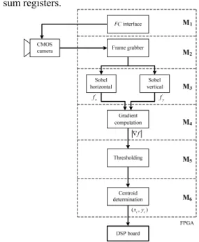
(3) applied to the image in Fig. 1 with the resulting image shown in Fig. 2.. Fig. 2. Edge detection using Sobel masks for the image in Fig. 1.. B. Thresholding Thresholding is a simple and efficient method applied to gray-level intensity images to differentiate between objects and the background in the image. Thresholding converts a gray-level image into a binary image that contains all of the essential information concerning the shape, position, and number of objects. Since we are interested in the lighter marker and the background is uniformly darker, global thresholding is used. The thresholding process is given by if f ( x, y )  T  255 fT ( x, y )   (4) if f ( x, y )  T 0 where T is the threshold value. Applying thresholding with a threshold value T  150 to the image of Fig. 2 produces the image in Fig. 3.. to configure the frame rate, gain control, exposure time, and integration time of the camera. M2: The frame grabber module acquires the pixels at a rate of 10 Mbytes/s from the camera. The image data can be directly passed to the next module. M3: This module consists of two parallel operations that realize Sobel edge detection using the horizontal and vertical mask operations (Equations (2) and (3)) to obtain the derivatives. Vertical and horizontal pixel counters are used to position the masks. M4: The sum of the absolute values of image derivatives is calculated to obtain the magnitude of the image gradient. The circuit synthesis requires an adder in this stage. M5: This module applies thresholding (Equation (4)) to the output image of the edge detection stage. M6: The centroid of the marker (Equation (5) and (6)) is calculated in this stage. The circuit synthesis requires two multipliers, three adders, two dividers, and three sum registers.. fx. Fig. 3. Thresholding applied to the image in Fig. 2.. f. C. Centroid and Displacement Determination Ideally, the thresholding operation separates the edge of the marker from the background and the pendulum rod of the scene. As shown in Fig. 3, the white pixels correspond to the edge of the marker. Because the marker is symmetrical, the centroid of the edge is taken as its location. The centroid ( xc , yc ) is given by xc .  x  f x.  f x. yc . T. ( x, y ). y. T. T. . f T ( x, y ). ( xc , yc ). Fig. 4. Parallel/pipelined architecture of FPGA.. IV. MODELING OF THE ROTARY INVERTED PENDULUM SYSTEM. ( x, y ). y. x. (5). y.  y  f x. ( x, y ). ,. fy. ,. (6). Consider the basic features of the rotary inverted pendulum system shown in Fig. 5.. y. where fT ( x, y ) represents the binary level of the pixel at point ( x, y ) in the image coordinate system. III. IMPLEMENTATION OF IMAGE PROCESSING ALGORITHMS ON AN FPGA In order to process the image data in real-time, the image processing algorithms introduced in the previous section are implemented on an FPGA using the hardware description language VHDL. In this study, the image processing is divided into the modules shown in Fig. 4. The functions of the modules are: M1: The Inter-Integrated Circuit (I2C) serial interface is used. m1 , l1 , c1. 2 m2 , l2 , c2. 1. l. Fig. 5. Rotary inverted pendulum system.. The variables and parameters of the system are defined as follows: m1 : Mass of the rotating arm (kg) m2 : Mass of the pendulum (kg).

(4) l1 : Length of the rotating arm (m) l2 : Length of the pendulum (m) C1 : Distance from the pivot point to the center of gravity of the rotating arm (m) C2 : Distance from the pivot point to the center of gravity of the pendulum (m) J1 : Moment of inertia of the rotating arm about the center of gravity (kg-m2) J 2 : Moment of inertia of the pendulum about the center of gravity (kg-m2) 1 : Angular displacement of the rotating arm (degrees)  2 : Angular displacement of the pendulum with respect to the vertical (degrees) g : Gravitational acceleration (m/s2)  l : Torque exerted on the rotating arm (N-m) The Euler-Lagrange formulation [23] was used to obtain the mathematical model of the system. It describes the dynamic behavior of the rotary inverted pendulum system. The model is M (q) q  Vm (q, q  q  G (q)    d , (7). where d is the disturbance torque, and   d    q   1 ,    l , d   1 , 0  2  d2   P  P sin 2  2 P3 cos  2  M (q)   1 2 , P4   P3 cos  2    P32 sin  2  1  Vm  q, q    2 ,  0  1  0   G q   ,   P sin 2  5. (8) (9) (10) (11). 1 P2 sin  2 2  . 2 The parameters Pi , i  1, ,5 are defined as. . P1  m2 l12  J 1 , P2  m2C22 , P3  m2l1C2 , P4  m2C22  J 2 , P5  m2C2 g. The relation between the force and control voltage is given by K K 2  l  m u  m , (12) Ra Ra. where  l is the control torque, u is the control voltage, K m is the motor constant and Ra is the armature resistance. TABLE II lists the physical parameters of the rotary inverted pendulum system. TABLE II Physical parameters of the rotary inverted pendulum system. Parameter m1 l1 C1 J1 Km g. Value 0.065 kg 0.16 m 0.08 m 0.00056 kg-m2 0.01376 N-m/A 9.8 m/s2. Parameter m2 l2 C2 J2 Ra. Value 0.022 kg 0.156 m 0.078 m 0.00017 kg-m2 1.08265 Ω. V. STABILIZING CONTROLLER DESIGN USING MIXED H 2 / H  CONTROL SYNTHESIS The rotary inverted pendulum system has two equilibrium points. The downward pendulum is a stable equilibrium point. The upward pendulum is an unstable equilibrium point. In order to design the stabilizing controller, the Jacobian linearized model is needed. First, the state variables are defined as T T x   x1 x2 x3 x4   1  2 1 2  . (13) Using the Jacobian linearization method [24], the dynamic equations (7) and (12) are linearized with respect to the unstable equilibrium [0, 0, 0, 0]T. The state-space equations of the linearized system are given by x1  x3 , (14) x2  x4 , (15) x3 . 1   P4 P6 x3  P3 P5 x2  P4 P7 u   P4 d1  P3 d 2 , L. (16). x4 . 1  P3 P6 x3  P1 P5 x2  P3 P7 u   P3 d1  Pd 1 2, L. (17). where K m2 K , P7  m . Ra Ra With the parameters from TABLE II, we obtain the state-space equations. The control objective is to stabilize the pendulum in the upright position. In this study, the measurement inaccuracy, quantization errors, and variance in illumination of visual measurements are regarded as white noise. The synthesis of the controller is formulated as a problem of the mixed H 2 / H  control. The H  norm constraint is used to enforce robustness against dynamic uncertainty, while the H 2 performance is used to ensure control effort, disturbance attenuation, and sensor noise attenuation. We introduce the vector of the measured output y  C y x  Dy w0 ,  L  P1 P4  P32 , P6 . where w0   d. n  is the exogenous input, d  R 2 is the T. torque disturbance as previously defined, and n  R is the visual sensor noise. The regulated output for H 2 performance is chosen to be z2  C2 x  D2 u. Thus, the open loop inverted pendulum model P is given by x  Ax  Bu  Bw w0 , z2  C2 x  D2u, y  C y x  D y w0 .. The control is given by an output-feedback controller K xc  Ac xc  Bc y, u  Cc xc  Dc y,. where xc  R and the matrices Ac , Bc , Cc , and Dc are of appropriate dimensions. A block diagram of the closed-loop system, which includes the linearized inverted pendulum nc.

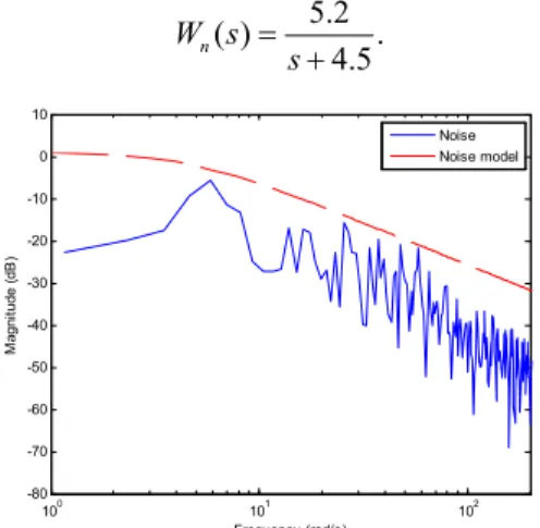
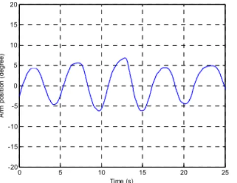
(5) model, the feedback controller, and the performance objectives, is shown in Fig. 6. z. 2. The H 2 norm of the closed-loop transfer function Twz2 from w to z2 is minimized to achieve the optimal H 2 performance. Let Wz ( s ) denote the transfer function matrix describing the frequency-domain characteristics for which the robustness is required. The H  norm of Wz KS  1 guarantees robust. Wz. . K. z2. Wn. n0. Fig. 6. Block diagram of the closed-loop system.. Here, we assume that the torque disturbance d is a unit impulse, which can represent the impulsive torque disturbance, such as a sudden tapping on the pendulum. The sensor noise n  Wn ( s ) n0 , where n0 is the white noise of zero mean and unit variance, and Wn ( s ) is the noise model. To determine the noise model Wn ( s ) , the visual sensor and an optical encoder are used to measure the angular displacement of the pendulum simultaneously. We assume that the measurement of the optical encoder is noise free. The sensor noise of the visual measurement is obtained by subtracting the measurement of the optical encoder from that of the visual sensor. Using FFT, we then obtain the frequency content of the noise, which is shown in Fig. 7. The frequency spectrum shown in Fig. 7 indicates that the noise from the visual sensor is colored. The noise model Wn ( s ) is selected to envelope the magnitude of the spectral content of the noise. It is given by 5.2 . Wn ( s )  s  4.5 10 Noise Noise model. 0 -10. Magnitude (dB). -20 -30 -40 -50 -60 -70 -80 0 10. 1. 2. 10 Frequency (rad/s). 10. Fig. 7. Frequency spectrum of the noise and frequency response of the noise model.. Let w  d. n0  , and denote the sensitivity function of the T. closed-loop system to be S   I  PK  . 1. The objective of the control design is to design a feedback controller K such that the closed-loop system is asymptotically stable. Moreover, the closed-loop system satisfies the following design specifications: 1. The closed-loop system guarantees robust stability against the additive plant uncertainty;. stability against the additive plant uncertainty. Thus, the above design specifications can be converted into a mixed H 2 / H  control design problem. That is to design a stabilizing controller K such that: min γ s.t. Wz KS  1 and Twz2   . . 2. The weighting function matrix 1 0 0 0    s  100  0 1 0 0  Wz ( s )  0.6 0.01s  100  0 0 1 0    0 0 0 1  is chosen to have high-pass characteristics to ensure robustness against plant uncertainty. The above mixed H 2 / H  control design can be cast into an LMI optimization problem [15] that can be solved in a numerically tractable manner. We use the MATLAB function hinfmix in the LMI Control Toolbox [28] to obtain a ninth-order controller. Note that the closed-loop performance and robustness of the system depends strongly on the selection of the weights Wn ( s ) and Wz ( s ) .. VI. EXPERIMENTAL RESULTS The designed control law and image processing algorithms were implemented and tested on the experimental setup shown in Fig. 8. The image processing algorithms were implemented on the FPGA board in VHDL. The designed robust controller was implemented on the DSP system in C. In this work, the camera can operate up to 580 frames/sec. However, the higher the frame rate, the stronger the intensity of light sources needed to ensure good quality of the acquired image. To overcome this difficulty, we lowered the frame rate to 250 frames/sec and installed three light emitting diodes near the top of the camera to provide the necessary intensity of light sources. The sampling frequency of the system was set to 250 Hz. The angular position responses of the pendulum and the rotating arm are shown in Fig. 9 and Fig. 10, respectively. The experimental results show that the designed visual servoing control robustly stabilizes the inverted pendulum system. To examine the robustness of the control system, an impulsive disturbance was manually added by tapping the pendulum at time 14 s (impulsive disturbance is indicated with D in Fig. 9). As shown in Fig. 9 and Fig. 10, the control system recovers from the impulsive disturbance..

(6) [2]. [3] [4] Fig. 8. Experimental setup. 10. [5]. D. 8. Pendulum position (degree). 6 4. [6]. 2 0 -2. [7]. -4 -6. [8]. -8 -10. 0. 5. 10. 15. 20. 25. Time (s). Fig. 9. Experimental result of the angular position response of the pendulum.. [9]. 20. [10]. 15. Arm position (degree). 10. [11]. 5 0. [12]. -5 -10. [13]. -15 -20. 0. 5. 10. 15. 20. 25. Time (s). [14]. Fig. 10. Experimental result of the angular position response of the arm.. The experimental results show that the system performs well even with noisy visual measurements and disturbance. A video that shows the balance control of the system is available at http://www.es.ncku.edu.tw/~csplab/Image RIP.mpg. VII. CONCLUSIONS In this paper, we reported the design and implementation of robust visual servoing control for balancing a rotary inverted pendulum. The image processing of the machine vision system was implemented on an FPGA device to meet real-time constraints. The robust controller was implemented through a DSP. The main contribution of this paper is twofold. First, the mixed H 2 / H  control was used to enhance the ability against plant uncertainty and noise due to image measurement. Secondly, the FPGA implementation was used to carry out image processing algorithms to achieve real-time constraints. The controller and the machine vision system were implemented and tested. Even with disturbance and sensor noise, the designed controller balanced the pendulum. REFERENCES [1]. S. Hutchinson, G. D. Hager, and P. I. Corke, “A tutorial on visual servo control,” IEEE Transactions on Robotics and Automation, vol.. [15]. [16] [17] [18] [19] [20] [21] [22] [23] [24] [25]. 12, no. 5, pp. 651-670, Oct. 1996. W. F. Xie, Z. Li, X. W. Tu, and C. Perron, “Switching control of image-based visual servoing with laser pointer in robotic manufacturing systems,” IEEE Transactions on Industrial Electronics, vol. 56, no. 2, pp. 520-529, Feb. 2009. Y. Motai and A. Kosaka, “Hand-eye calibration applied to viewpoint selection for robotic vision,” IEEE Transactions on Industrial Electronics, vol. 55, no. 10, pp. 3731-3741, Oct. 2008. S. M. Bhandarkar, X. Luo, R. F. Daniels, and E. W. Tollner, “Automated planning and optimization of lumber production using machine vision and computed tomography,” IEEE Transactions on Automation Science and Engineering, vol. 5, no. 4, pp. 677-695, Oct. 2008. T. Bucher, C. Curio, J. Edelbrunner, C. Igel, D. Kastrup, I. Leefken, G. Lorenz, A. Steinhage, and W. von Seelen, “Image processing and behavior planning for intelligent vehicles,” IEEE Transactions on Industrial Electronics, vol. 50, no. 1, pp. 62-75, Feb. 2003. J. Batlle, J. Marti, P. Ridao, and J. Amat, “A new FPGA/DSP-based parallel architecture for real-time image processing,” Real-Time Imaging, vol. 8, no. 5, pp. 345-356, Oct. 2002. J. Diaz, E. Ros, F. Pelayo, E. M. Ortigosa, and S. Mota, “FPGA-based real-time optical-flow system,” IEEE Transactions on Circuits and Systems for Video Technology, vol. 16, no. 2, pp. 274-279, Feb. 2006. Y. Yoon, A. Kosaka, A. C. Kak, “A new Kalman-filter-based framework for fast and accurate visual tracking of rigid objects,” IEEE Transactions on Robotics, vol. 24, no. 5, pp. 1238-1251, Oct. 2008. D. S. Bernstein and W. M. Haddad, “LQG control with an H∞ performance bound: A Riccati equation approach,” IEEE Transactions on Automatic Control, vol. 34, no. 3, pp. 293-305, Mar. 1989. P. P. Khargonekar and M. A. Rotea, “Mixed H2/H∞ control: A convex optimization approach,” IEEE Transactions on Automatic Control, vol. 36, no. 7, pp. 824-837, Jul. 1991. S. Boyd, L. El Ghaoui, E. Feron, and V. Balakrishnan, Linear Matrix Inequalities in Systems and Control Theory, SIAM studies in applied mathematics, SIAM, Philadelphia, PA, 1994. L. El Ghaoui and S. I. Niculescu, editors, Advances in Linear Matrix Inequality Methods in Control, Advances in Control and Design, SIAM, Philadelphia, PA, 2000. L. Vandenberghe and V. Balakrishnan, “Algorithms and software for LMI problems in control,” IEEE Control Systems Magazine, pp. 89-95, 1997. C. W. Scherer, “Mixed H2/H∞ control,” Trends in Control, A European Perspective, A. Isidori, Ed., pp. 173-216, Berlin: Springer-Verlag, 1995. C. W. Scherer, P. Gahinet, and M. Chilali, “Multiobjective output feedback control via LMI optimization,” IEEE Transactions on Automatic Control, vol. 42, no. 7, pp. 896-911, Jul. 1997. X. Huang and R. Horowitz, “Robust controller design of a dual-stage disk drive servo system with an instrumented suspension,” IEEE Transactions on Magnetics, vol. 41, no. 8, pp. 2406-2413, Aug. 2005. C. Du, L. Xie, J. N. Teoh, and G. Guo, “An improved mixed H2/H∞ control design for hard disk drives,” IEEE Transactions on Control Systems Technology, vol. 13, no. 5, pp. 832-839, Sep. 2005. M. E. Magana and F. Holzapfel, “Fuzzy-logic control of an inverted pendulum with vision feedback,” IEEE Transactions on Education, vol. 41, no.2, pp. 165-170, May 1998. H. Wang, A. Chamroo, C. Vasseur, and V. Koncar, “Hybrid control for vision based cart-inverted pendulum system,” Proceedings of 2008 American Control Conference, pp. 3845-3850, Jun. 2008. O. Faugeras, Three Dimensional Computer Vision, MIT Press, 1993. Y. Ma, S. Soatto, J. Kosecka, and S. Sastry, An Invitation to 3-D Vision: From Images to Geometric Models, Springer, 2003. R. C. Gonzalez and R. E. Woods, Digital Image Processing, Prentice Hall, Upper Saddle River, NJ, 2002. H. Goldstein, C. Poole, and J. Safko, Classical Mechanics, Addison Wesley, Upper Saddle River, NJ, 2002. H. K. Kahlil, Nonlinear Systems, Prentice Hall, Upper Saddle River, NJ, 2002. P. Gahinet, A. Nemirovski, J. A. Laub, and M. Chilali, LMI Control Toolbox for Use with MATLAB, The Mathworks Inc., 1995..

(7)