A state-space approach to the multivariable continuous-time self-tuning control

(1)

WM3

-

2 5 0

A

State-Space Approach To

The Multivariable Continuous-Time Self-Tuning

Control

Min-Shin Chen* and Yi-Hsiang Huang

t

Department of Mechanical Engineering

National Taiwan University

Taipei, Taiwan, Republic

of

China

FAX

:

886-2-3631755

Abstract

In this paper, we propose a new self-tuning control for continuous-time linear time invariant MIMO systems. We first develop a self-tuning multi-input state feedback control, and then develop a self-tuning control for a general MIMO system with an input- output description. In the latter case, we show that once the system's dynamics of the MIMO system is properly parameterized into a nonminimal state space description, the self-tuning control problem can be transformed into that in the former case, and therefore be solved similarly. The unique feature of our state space approach compared with the conventional polynomial equation approach is that the only a priori information on the system required is an upper bound of the system's observability indices.

Section I Introduction

In this paper, we propose a new continuous-time self-tuning controller for general continuous-time systems. Our approach differs from previous approaches in two aspects: (1) Previous approaches rely on a pa- rameterization using polynomial equations. In our ap- proach, we use a state space parameterization, and start the design with the self-tuning state feedback control in which the system state is accessible for mea- surement. We then show that the proposed design procedure can be applied to the more general case in which the system is described in polynomial equations and only the system's outputs are accessible for mea- surement. This new approach enables us to design STC's for MIMO systems without substantial efforts compared with the SISO systems. (2) We need only the knowledge of an upper bound of the system's observability indices for the STC design - a more re- laxed assumption on the system than previous results.

*Associate professor

t

Graduate Student

Section I1 Preliminaries

The following lemmas will be used to establish the stability of the self-tuning controller presented in this paper. They are either well known in the adaptive control theory or can be easily derived from others; their proofs are relegated to the references.

Lemma 1 [l] : Let w : R+ 4

R"

be piecewise con-

tinuous, @ = @

-

@, where @ is an unknown constant vector, and e = @'W. If and - = - d P d t 1

+

y w T P w g P w w T P

,

p ( 0 ) = P ( t S ) = ko . I > 0,

where y and g are positive constants, t , =

{ t

I

Xmin(P(t))

5

kl

<

ko}. Then

( i ) @ . E L ,

,

8 E L z n L m ,

emm ma-2

121 : Swapping lemma. Let

8,

u : R+ --*

R"

and B be differentiable. Then

(8'")f

= P U f

-

( h f ) f ,

where the subscript

f

denotes the filtering process:

"f

=

-

x > o .

S + X W '

In the following lemmas, H ( s ) is the rational transfer function of a strictly proper and asymptotically stable system.

Lemma 3 [3] : Let y = H ( s ) u , then there exists a positive constant

M

such that

(2)

Iy(t)l

5

MIIutll,+exponentiaZ~y decaying term. Lemma 4 [3] : Let y = H ( s ) u , and u ( t )

E

L1 or

Lz.

Then y ( t ) + 0 as t + 00.

Lemma 5 [3] : Let y = H ( s ) ( p u ) , where p ( t ) E LZ

or L1 and u ( t )

E

L w e . Then there exists a continuous function

p ( t )

such that p ( t )

-

0 as

t

-

00 and

y ( t ) = ,8(t)llutllw

+

exponentially decaying term.

Combining Lemmas 2 , 3 and 5, we obtain the fol- lowing corollary.

Corollary: Consider Lemma 2 again with

e^

E

LZ

and v

E

L m e . We have

(eT+

= d T V f

+

a ( t ) l l v t / l m ,

where a ( t ) -+ 0 as

t

-+ 00.

Lemma 6 [4] : Let D ( s )

E

RpxP[s], the set of p x p

matrices with polynomial elements, and & D ( s ) denote the maximum.po1ynomial degree in the i-th row of

D ( s ) . There exists a real p x p matrix r D such that : D ( s ) = s D ( s ) r D + T D ( s )

where & T D ( s )

<

a , D ( s ) , and S D ( S ) is a diagnoal ma- trix with seiD(') as the i-th element on the diagnal.

Lemma 7 [4] : Let P ( s )

E

Rmxm(s), the set of m x

m matrices whose elements are rational functions of

s. Let N L ( s ) and D L ( s )

E

Rmxm[s]

be such that

P ( s )

= D ( s ) - l N ( s ) . If D ( s ) is row reduced, then P ( s ) is strictly proper iff & N L ( s )

<

& D L ( S ) for all

1 m .

i = 1,

...

Section

I11

Self Tuning LQR Control

Consider a linear time invariant system

E = ( A

+

A A ) z

+

(B

+

A B ) u , (3.1) where

x

E

R"

denotes the state vector, U

E

R"

the input vector, ( A , B) the nominal system matrices, and

( A A , A B ) the unknown system matrices. We assume that the system state x is directly accessible. The objective now is to estimate the unknown system matrices, and apply the certainty equivalence principle [5] to the design of a regulation controller. In this paper, we demonstrate the control design using the opti- mal state feedback controller; however, other types of linear controllers, static or dynamic, can also be em- ployed without affecting the results obtained below.

Section 1II.A Parameters Identification

To identify the uncertain parameters in the system, we reparameterize the system dynamics (3.1) as fol- lows: define

f ( s ) = s + X ,

x > o

(3.2)

and divide the Laplace transform of Eq.(3.1) by f(s), obtaining

S Z ~ = A z ~

+

Buj

+

A A z f

+

A B u ~

+

- (3.3)

S + X '

where we have set the initial conditions of zf and u f to be zeros with

(3.4) Rearranging the inverse Laplace transform of Eq.(3- .3), and looking at the equation rowwisely, we find

@Tuf = - - ~ z ! i +z,

-

~ , z f

-

Biuf

-

z i ( 0 ) e - x t , (3.5) where OF = ( A A i , A B i ) ,

UT

= ( x f , u f ) , and i =

1 , 2 , .

. .

, n . Denote the parameter error

ai

= Oi

- 6i3

where

6T

= ( A A * , A & ) is an estimate of O i , we define the identification error

e , = aTvj

= - - X x f i + ~ , - A i z f - B i u f - ~ i ( O ) e - ' ~ - 6 i v f , (3.6) where we used Eq.(3.5) to obtain the second equality. Based on Eq.(3.6), we apply the normalized L.S. algorithm in Lemma 1 to update 0 , resulting in

(i)

ai E

L ,

,

bi

E LZ

nL,,

(3.7)

E

L~

n

L,.

(3.8) QTvf 1

+

IIVftll,

(ii)

pi = f o r a l l i = 1 , 2

,...,

n.

Section 1II.B Controller Design

Having obtained an estimate of the unknown system parameters, we can construct different types of controllers based on the estimated system ( A

+

A A ,

B

+ A B ) . In particular, we choose the LQR controller in this paper. The control input is then given by

=

- K x , K

= R - I B T P (3.9) where

P

is the positive definite solution of the Riccati equation :

A T F + P A + Q - P B R - ' B T F = 0, Q , R

>

0 (3.10) with

A

= A

+

A A , B = B

+

A B , and

( A ,

B )

stabi- lizable by Assumption ( A l ) . The closed-loop system dynamics then becomes

i

= [ A + A A - ( B + A B ) ~ ; ~ ~ = [ A

+

A A

-

( B

+

AB)^+

+ [ ( A A

-

A A )

-

( A B

-

AB)&lilz

= A K - x + a v (3.11)

where

AK

=

A

-

B k ,

aT

= (@I

,...,

a,,),

and vT = ( x T , u T ) . Notice that Eq.(3.11) represents a

(3)

typical result for almost all types of self-tuning control systems: the first term of the right-hand side r e p resents the desired system dynamics if the estimated parameters all converge to their true values; the second term represents a perturbation to the desired system due t o the identification error.

Section 1II.C Stability of the Self Tuner

In this subsection, we will show that as long as there exists a Lyapunov function for the exact nonadaptive controller, the asymptotic convergence of the state variables can be established for the self-tuning controller using the original Lyapunov function.

Proof: Divide the Laplace transform of Eq.(3.11) by f(s), and take the inverse Laplace transform of the equation, we obtain

if

= (AKz)f

+

( o T v ) j

+

z(O)e-"

Since 21, wf E L,, and

&,

A k E L Z (see Eq.(3.7), we apply the Corollary in Section I1 to obtain

X f = A K Z f

+

a Y l ( t ) l l Z f t l l w

+

Q T V f

+

aZ(t)llwftllw (3.12) where a l ( t ) and az(t) -+ 0 as t -+ m and the expo-

nentially decaying term z ( 0 ) e - x t has been absorbed into the last term. Using Eq.(3.8) and the fact that llvftllm

5

Nllzftllw for some positive constant N ,

Eq.(3.12) can be rewritten as

=

A K Z ~

+a3(t)llzft 1100 + P i (t)(1+112jtllm) (3.13)

where ad(t) -+ 0 as t -+ m and P i ( t )

E

Lz.

Define V =

Z T P Z ~ ,

where

f

'

is the solution of the Riccati equation in Eq.(3.10). Note that this V ( z j )

function is a valid Lyapunov function for the exact nonadaptive system

X f = A K Z f ,

when all the system parameters are fixed. In our case of self-tuning controllers,

P

is time-varying. However, we will show that this V ( t , z f ) function can still be used to verify the convergence of the state variables. Taking the time derivative of V function along the tra- jectory :i Eq.(3.13), and noticing that the time derivative of

P

is in

L z ,

we obtain

v

= Z T P X f

+

zTPz,

+

k T P Z f +a311zftllw)

+

Z T P Z f

5 -0v

+

P 2 ( 9 4 i E i L +

P 3 ( ~ ) l l v t l l m = X T ( P A K

+AgP)zf

+

2ZTp(Pl(1

+

I I Z f t l l w ) + a 4

(t)llvt

llw

+

P4(t)llvtllw, where 0

=

**inft~o(mi.XIQ+PBR-lB*~]),**

a 4 ( t ) -+ 0 as t -+ 00, and

,&,

/ 3 3 , P 4

E

Lz.

Combining /33 and P 4

into /35, and integrating the above inequality from 0

to t gives:

where I'l(t), I' z ( t ) and I'3(t) approach zeros as t -+ 00

by Lemma 4. The last inequality enables us t o conclude that V(t) -+ 0 as t --* 00. This can be seen as fol-

lows: assume that limt,,V(t) -+ 00; in other words,

there exists an infinite sequence { t i , i =

. .

,

m)

such that 1

<

V ( t i )

=

~ ~ v t ( t i ) ~ ~ m and limi-wV(ti) -+

W . Equation (3.14) then suggests that

1

i

r i ( t i )

+

r z ( t i )

+

r 3 ( t i )

Since the right-hand side of the last inequality ap- proaches zero as

i

-+ 00, a contradiction is obtained.

We then conclude that V(t) is bounded; i.e., there exists aconstant M such that

llVtllm

5

M for all t 2 0 .

Again, inequality (3.14) suggests that

~ ( t )

5 m(rl(t)

+

rz(t))

+

A T r 3 ( t )

Since ri's all approach zeros as t -+ 00, V ( t ) and zf

also approach zeros as t -+ 00.

It remains to show that the state variables z ( t ) a p proach zero asymptotically. To show this, we divide Eq.[3.9) by f(s), and notice that the time derivative of

K

belongs to L 2 ,

"f

=

-(k+

=

- k Z f

+

a 5 ( t ) l l Z f t l l w , (3.15)

where we have used the Corollay again t o obtain the second equality, and a 5 ( t ) -+ 0 as t -+ 00. Since

z f approaches zero, so does u t . From the definition of w T = ( % f l u ! ) , wf also approaches zero. Finally, according to Eqs.(3.4) and (3.12),

2

= if

+

X C f

= A K Z f

+

al(t)llCftllw

+

o T V f

+

Qz(t)llvftllw

+

X Z f .

We can now conclude that ~ ( t ) approaches zero asymptotically.

(4)

Consider a strickly proper MIMO system

[ D ( s )

+

A D ( s ) ] y = [ N ( s )

+

A N ( s ) ] u (4.1)

D ( s ) , A D ( s ) , N ( s ) , A N ( s ) E R m x m [ s ]

where y is the system output, U the control input, D ( s )

and N ( s ) are known a priori, and A D ( s ) and A N ( s )

denote the uncertain parts of the system dynamics, and D ( s ) ( + A D ( s ) ) and N ( s ) ( + A N ( s ) ) are coprime. By Lemma 6. we can write

D(S)

+

AD(S) = S D + A D ( s ) r D + A D

+

T D + A D ( s )

where & T D + A D ( ~ )

<

& ( D ( s )

+

A D ( s ) ) , and S D + A D ( S ) is a diagonal matrix with sBi(DtAD) as the i-th element on the diagonal. Without loss of gener- ality, we assume that

D ( s )

+

A D ( s ) is row-reduced;

r D + A D is therefore nonsingular. Note that since

( D ( s )

+

A D ( s ) ) - ' ( N ( s )

+

AN(s)) is strictly proper, we have 0

5 & ( N

+

A N )

<

& ( D

+

A D ) by Lemma 7; hence, the observability index vi = a i ( D

+

A D )

2

1,Vi. We assume that an upper bound of the observability index of D(s)+A D ( s ) ,

~ ( 2

v i ) , is known in advance. Instead of developing an identifier for uncertain parameters in A D ( s ) and A N ( s ) directly based on Eq.(4.1), we will obtain a nonminimal state-space realization of the systems, estimate unknown parameters in this state-space realization, and then follow the approach developed in Section I11 to construct the self-tuning controller.

The state variables of the proposed nonminimal realization are defined by

Z

= [ y i ,

....

y m , ~ 1 1 , .

. . .

zlm, 1 2 1 , .

...

zzm] E R2"("-')+",

where 21, and 2 2 , satisfy

21, = A z ~ i

+

P y i , kzi = Azz,

+

Pu,,

i = 1 .

..

m

( 4 4

h ( s ) = s7-l

+

h , - ~ s " ' - ~

+

. . .

+

ho is any Hurwitz and the characteristic equation of A E R("")'("-') :

polynomial.

Let Q(s) be a polynomial matrix such that

a i Q ( s ) = q-vi for i = 1

...

m , and detQ(s) be a monic Hurwitz polynomial; in other words, we restrict that

re

= I . One such selection can be Q(s) = diag[(s

+

detQ(s) equals X i = ' ( q - v i ) = m e q - x v i = m 9 - n . Multiply Q ( s ) on both sides of Eq.(4.1),

Q(s) [ D ( s )

+

A D ( s ) ] y = Q ( s ) [ N ( s )

+

A N ( s ) ] u

. . . .

(s

+

a):-Ynz]. We notice that the degree of

[b(s)

+

A 6 ( s ) ] y = [fi(s)

+

A f i ( s ) ] u (4.3) where b ( s ) = Q ( s ) D ( s ) and A b ( s ) , f i ( s ) , A f i ( s ) are similarly defined. The system in (4.3) is still strictly proper; hence, according to Lemma 7, for i

=

1 .

. .

m ,

we have

&(fi

+

A i )

<

&(b

+

A d ) . (4.4)

Since

re

= I , we have

Sfi+Afi = 3" * I (4.5)

rfi+afi = r D + A D ( 4 4

Pick H ( s ) = h ( s )

.

r D + A D , where h ( s ) is the char-

acteristic equation of A in Eq.(4.2). Since h ( s ) is of degree q

-

1, we have

S H = s"-'

.

I (4.7)

r H = r D + A D (4.8)

Divide Eq.(4.3) by H ( s ) , obtaining

H - ' ( s ) [ ~ ( s ) + A b ( s ) ] y = H - ' ( s ) [ f i ( s ) + A ~ ( s ) ] u

Because of Eqs.(4.5)~(4.8), the left-hand side of Eq.(4.9) posesses only one nonproper term s

.

I , and

all terms on the right-hand side of Eq.(4.9) are proper. Shifting all the proper terms to the right-hand side of the equation, Eq.(4.9) can be rewritten as, in terms of the time-domain signals,

(4.9)

Y

=

(eo

+

A O ~ ) ~ Y +

(el

+

a q T t l

+(IC

+

~ k b

+

(ez

+

zz

+exponentially decaying term (4.10)

where nominal matrices k E R""", 00 E R m x m ,

81,82 E Rm("-m)xm are obtained from b ( s ) and

fi(s), and uncertain matrices Ak E Rmxm-, A60

E

Rmxm

,

A81, A& E R"("-"')'" f rom A D ( s ) and

A f i ( s ) .

We further stack Eqs(4.2) and (4.10) to obtain

z

= FZ+GU =

( F

+

A F ) Z

+

( G

+

AG)u (4.11) y = H Z . where

.

_.

.

_.

.

_.

.

. . .

...

p 0 0 . :. a 1 0

. . .

F = l 0 0 . . . 0 0 0 . . . O l A 0 . . . 0 . . . 0 0 . . .

.

. . . . .

. . .

1:

0

. . .

0 0

. . .

A F = , G = 0 0 0 . . k 0

. . .

0 . . . .

.

_.

.

_.

.

0

. . .

0 /3 0 " ' 0 0 p " ' 0 . . . . . . . . . . . . . . 0 B 0 1 A / A G T = ( A k 0 0 ) , H = ( I 0 0 )

In developing the realization in Eq.(4.11), we have used Q(s) and H ( s ) whose choices require the knowledge of the system's observability indices and the constant matrix r D + A D , so that we can find the nominal

(5)

matrices (F, G). However, suppose that we have no information a t all on the system’s parameters((F, G) = 0), the application of the proposed control requires only the knowledge of an upper bound of the observability indices for the determination of the dimension of the filtering process in Eq.(4.2). There would be no need to know O(s) and H ( s ) to apply the control, and Assumption (B2) is guaranteed.

Notice that the system state 2 in Eq.(4.11) is read- ily accessible as indicated by Eq.(4.2). We can there- fore follow the approach in Section I11 to construct a self tuning controller for the system in Eq.(4.11). The design procedure and stability proof are exactly the duplicates of those in Section 111, and are omitted. Here, we merely use a simulation example to demonstrate the results.

Example Consider a system

2 S , ,

.

, ,

.

‘ , ‘ , 2 ...

....

Act!.. ... ~ 1.5

::

3 i E

,i

B

i

AG,, * . . B 5

2

0.5 ~ APB. AY,# ... 0 ... 6

...

4 . 5 ~

/ o

-1 0 0

\

/ o

1 \ l o

Its transfer function matrix is described as

2 4 6 n io 12 14 i 6 i n 20

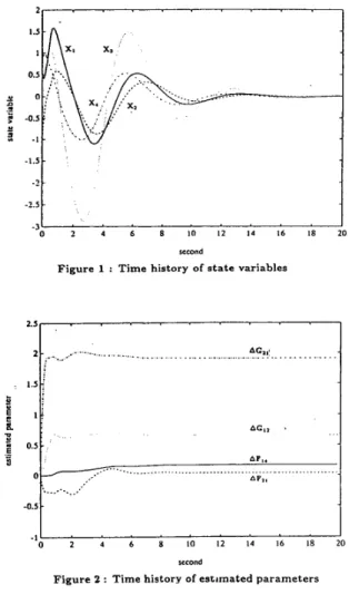
Suppose that the nominal system (F, G) = 0, we con- struct the self-tuning controller as developped in this Section with 9 = 3, h ( s ) = sz

+

4 s

+

3 in Eq.(4.2), f ( s ) = s

+

5 in Eq.(3.2), Q = diag(l0,10,5,...,5) and R = 20

.

Z in Eq.(3.10). We use the normalized L.S. algorithm for estimation of ( A F , A G ) with

PL(O)

= 1 0 . I, g = 10, y = 1. All the state variables are successfully regulated to zero as shown in Figure

1, and the deviations of four of the estimated parameters from their initial guesses are shown in Figure 2. We note t h a t in this example, altogether there are 20 estimated parameters while we showed only four of them.

References

[l] G. C. Goodwin and D. Q. Mayne, ” A Parame-

ter Estimation Perspective of Continuous Time Model Reference Adaptive Control”, Automatica, vol. 23, no. 1, pp. 57-60, 1987.

[2] S. SASTRY and M. BODSON, Adaptive Control

: Stability, Convergence, and Robustness, Prentice-

Hall, New Jersey, 1989.

[3] Kumpatis Narendra, Yuan-Hao Lin and benas Valavani ”Stable Adaptive Controller Design, PART I1 : Proof of Stability,” IEEE Trans. Automat. Contr., vol. AC-25, pp. 440-449, JUNE, 1980.

[4] M.

D.

Mathelin and M. Bodson, ”Parameter Con- vergence in Multivariable Recursive Identification,” Laboratory for Automated Systems and Information Processing. Electrical and Computer Engineering De- partment, Carnegie Mellon University, Pittsburgh, PA [5]

K.

J. Astrijm,

U.

Borisson, L. Ljung and B. Wit- tenmark, ”Theory and application of self-tuning reg- ulators,” Automatica, vol. 13, pp. 457-476, 1977. 15213-3890, USA.

sewnd